Báo cáo hóa học: " Research Article Quadratic Interpolation and Linear Lifting Design" docx

Hindawi Publishing Corporation
EURASIP Journal on Image and Video Processing
Volume 2007, Article ID 37843, 11 pages
doi:10.1155/2007/37843

Research Article
Quadratic Interpolation and Linear Lifting Design
´
Joel Sole and Philippe Salembier
Department of Signal Theory and Communications, Technical University of Catalonia (UPC), Jordi Girona 1–3, Edifici D5,
Campus Nord, Barcelona 08034, Spain
Received 11 August 2006; Revised 18 December 2006; Accepted 28 December 2006
Recommended by B´ atrice Pesquet-Popescu
e
A quadratic image interpolation method is stated. The formulation is connected to the optimization of lifting steps. This relation
triggers the exploration of several interpolation possibilities within the same context, which uses the theory of convex optimization to minimize quadratic functions with linear constraints. The methods consider possible knowledge available from a given
application. A set of linear equality constraints that relate wavelet bases and coefficients with the underlying signal is introduced
in the formulation. As a consequence, the formulation turns out to be adequate for the design of lifting steps. The resulting steps
are related to the prediction minimizing the detail signal energy and to the update minimizing the l2 -norm of the approximation
signal gradient. Results are reported for the interpolation methods in terms of PSNR and also, coding results are given for the new
update lifting steps.
Copyright © 2007 J. Sol´ and P. Salembier. This is an open access article distributed under the Creative Commons Attribution
e
License, which permits unrestricted use, distribution, and reproduction in any medium, provided the original work is properly
cited.

1.

INTRODUCTION

The lifting scheme [1] is a method to create biorthogonal

wavelet filters from other ones. Despite the amount of research effort dedicated to the design and optimization of lifting filters since the scheme was proposed, many works (p.e.,
[2–4]) that contribute ideas to improve existing lifting steps
with new optimization criteria and algorithms keep appearing. Certainly, there is room for contributions, specially in
space-varying, signal-dependant, and adaptive liftings. Even
in the linear setting, there are lines that deserve a further
study. This paper follows the works [5, 6]. It proposes a linear
framework for the design of lifting steps based on adaptive
quadratic interpolation methods. First, a family of interpolation methods is presented. The interpolation is employed
for the design of prediction and update lifting steps. It is assumed that an improvement in the interpolation implies an
improvement in the subsequent lifting steps.
The prediction step extracts the redundancy existing in
the odd samples from the even samples, so interpolative
functions are a reasonable choice as initial prediction lifting
steps. An adaptive quadratic interpolation method is proposed in [7], which is outlined in Section 2. The interpolation signal is found by means of the optimal recovery theory.
We have observed that the problem statement may be reformulated as the minimization of a quadratic function with

linear equality constraints. This insight provides all the resources and flexibility coming from the convex optimization
theory to solve the problem. Furthermore, the initial problem statement may be modified in many different ways and
the convex optimization theory still offers solutions. These
variations are presented in Section 3.
This flexibility also allows the design of lifting steps with
different criteria than the usual vanishing moments and
spectral considerations. First, linear constraints are changed.
Transformed coefficients are the inner product of wavelet
basis vectors with the signal data. These products are new
linear constraints introduced in the formulation. This fact
permits the construction of initial prediction steps as well
as the subsequent prediction and update steps for which
the spatial interpolation interpretation is not straightforward.
Sections 5 and 6 present the design of prediction and

update steps, respectively. Experiments are explained in
Section 7. Results for the different interpolation methods
are given in a setting linked to the lifting scheme. Lifting
steps performance is assessed by means of the bit rate of
compressed images. Finally, main conclusions are drawn in
Section 8.
Notation 1. Boldface uppercase letters denote matrices, boldface lowercase letters denote the column vectors, uppercase


2

EURASIP Journal on Image and Video Processing

italics denote sets, and lowercase italics denote scalars. Indexes are omitted for short when they are clear from the context.
2.

0

1

2

3

4

5

6

7

0
1
2

QUADRATIC INTERPOLATION

3

An adaptive interpolation method based on the quadratic
signal class determined from the local image behavior is presented in [7]. We reformulate the method and propose several variations on it that consider additional knowledge available from the application at hand.
The described methods are based on two steps. First, a set
to which the signal belongs (or a signal model) is determined.
Second, the interpolation that best fits the model given the
local signal is found. The first step is common for all the
methods, whereas the second one is modified according to
the available information. This section presents the first part
and derives an optimal solution. This initial solution is retaken in Sections 5 and 6 with the goal of designing lifting
steps. Section 3 describes alternative formulations.
A quadratic signal class K is defined as K = {x ∈
Rn : xT Qx ≤ }. The choice of a quadratic model is practical because it can be easily determined using training data.
The quadratic signal class is established by means of m image patches S = {x1 , . . . , xm } representative of the local data.
Patches may be extracted from an upsampling and filtering
of the image or from other images. Patches are high density,
that is, they have the same resolution as the interpolated image. Therefore, if patches are extracted from the image to be
interpolated, then an initial interpolation method is required
and the proposed methods aim at improving the initial result.
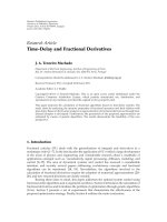
Figure 1 depicts an example of image to be interpolated
(the black pixels), and the high-resolution image (which includes the light pixels). The training set has to be selected.

One direct approach of selecting the elements in S is based
on the proximity of their locations to the position of the vector being modeled. In this case, patches are generated from
the local neighborhood. For example, in Figure 1 the center
patch
x = x(2,2) x(2,3) x(2,4) x(2,5) x(3,2) · · · x(5,5)

T

(1)

may be modeled by the quadratic signal class of the set
⎞
⎛
⎞⎫
⎧⎛
x(4,4) ⎪
⎪ x(0,0)
⎪
⎪
⎪
⎜x
⎟⎪
⎪⎜x(0,1) ⎟
⎪
⎨⎜
⎟
⎜ (4,5) ⎟⎬
⎜ . ⎟,...,⎜ . ⎟ ,
S = ⎪⎜ . ⎟
⎜ . ⎟⎪

⎪⎝ . ⎠
⎝ . ⎠⎪
⎪
⎪
⎪
⎪
⎩
⎭

x(3,3)

(2)

x(7,7)

where S is formed by choosing all the possible 4 × 4 image
blocks in the 8 × 8 region of the figure.
Matrix S is formed by arranging the image patches in S
as columns: S = (x1 · · · xm ). The solution image patch x
is imposed to be a linear combination of the training set S
through a column vector c:
Sc = x.

(3)

4
5
6
Center patch

7

Figure 1: Local high density image used for selecting S to estimate
the quadratic class for the center 4 × 4 patch (dark pixels are part of
the decimated image).

As discussed in [7], vectors in S are similar among themselves and x is similar to the vectors in S when c has small
energy,
c

2

= cT c = xT SST

−1

,

x≤ .

(4)

In this sense, good interpolators x for the quadratic class determined by (SST )−1 are expanded with the weighting vectors
c of energy bounded by some .
Once the high density class S is determined, the optimal
interpolated vector x can be simply seen as the solution of
a convex optimization problem, instead of using the optimal
recovery theory as in [7]. We are looking for the vector c with
minimum energy that obtains an interpolation x that is a linear function of the patches. This statement can be formulated
as

minimize

c 2,

subject to

Sc = x.

x,c

(5)

Without any additional constraints, the optimal solution of
(5) is x = 0 and c = 0. The information coming from the
signal being interpolated should be included in the formulation to obtain meaningful solutions. Previous knowledge
about x is available since only some of its components have
to be interpolated. Typically, if a decimation by two has been
performed in both image directions, then one of every four
elements of x is already known (the black pixels in Figure 1).
Another possible case is the following: it may be known that
the original high density signal has been averaged before a
decimation. In both cases, a linear constraint on the data is
known and it may be added to the formulation (5). The linear constraint is denoted by AT x = b. In the first case, the
columns of matrix A are formed by canonical vectors ei , being the 1’s located at the position of the known sample. The
respective position of vector b has the value of the sample.
An illustrative example for the second case is the following.
Assume that the pixel value is the average of four high density neighbors, then there would be 1/4 at each of their corresponding positions in a column of A. Whatever the linear


J. Sol´ and P. Salembier

e

3

constraints, they are included in (5) to reach the formulation,

by 0 and up-bounded by 2nbits − 1. This is an additional constraint that may be included in the problem statement as

c 2,

minimize
x,c

c 2,

minimize

subject to Sc = x,

x,c

(6)

subject to Sc = x,

AT x = b.

0 ≤ x ≤ 2nbits − 1 · 1,

The solution of this problem is

x = SST A AT SST A

−1

b,

(7)

which is the least square solution for the quadratic norm determined by SST and the linear constraints AT x = b.
Note that the solution vectors can be seen as new data
patches, better in some sense than the originally used by the
algorithm. These solution vectors may be provided to a subsequent iteration of the algorithm, thus improving initial results.
Taking the expectation in (7), the formulation can be
made global. In this case, the quadratic class is determined
by the correlation matrix R = E[SST ]. The equivalent global
formulation of (6) is
minimize
x

subject to AT x = b

(8)

and the corresponding solution is
−1

b.

(9)

To sum up, this formulation is useful to construct locally
adapted as well as global interpolations. Global interpolation
means that a quadratic model (via the autocorrelation matrix) is used for the whole image. If local data is available, the
example patches are a good reference for the local quadratic
interpolation.
Additional knowledge may easily be included in the formulation thanks to its flexibility. In the next section, several
alternative formulations are proposed that modify the presented one in different ways.
3.

where 0 (1) is the column vector of the size of x containing all
zeros (ones). The symbol ≤ indicates elementwise inequality.
Let us define the set
D = x ∈ Rn | 0 ≤ x ≤ 2nbits − 1 · 1 .

ALTERNATIVE FORMULATIONS

The initial formulation (6) and its solution give a good interpolation, which is optimal in the specified sense. However, the problem statement may be further refined including additional knowledge, from the local data or from the
given application. Knowledge is introduced in the formulation by modifying the objective function or by adding new
constraints to the existing ones. Various alternative formulations are described in the following.
3.1. Signal bound constraint
The data from an image is expressed with a certain number
of bits, let us say nbits bits. Then, assume without loss of generality that the value of any component of x is low-bounded

(11)

Notice that (10) is a quadratic problem with inequality linear
constraints and so, it has no closed-form solution. Anyway,
there exist efficient numerical algorithms [8] and widespread
software packages (p.e., Matlab) that attain the optimal solution fast. However, if the optimal solution x of (10) resides
in the bounded domain D, then a closed-form solution exists and is expressed by (7).

3.2.

xT R−1 x,

x = RA AT RA

(10)

AT x = b,

Weighted objective

Another refinement of (6) is to weight vector c in order to
give more importance to the local signal patches that are
closer to x. Closer patches are supposed to be more alike than
the further ones. The formulation is
minimize
x,c

Wc 2 ,
(12)

subject to Sc = x,
AT x = b,

where W is a diagonal matrix with the weighting elements
wii related to the distance of the corresponding patch (in the
column i of S) to the patch x. Let us denote W = WT W, then
the problem may be reformulated as
minimize

c

cT Wc,
(13)

subject to AT Sc = b,

which is solved using the Karush-Kuhn-Tucker (KKT) conditions [8, page 243]:
⎧
⎨AT Sc − b = 0,

KKT conditions: ⎩
2Wc + ST A μ = 0,

(14)

which are equivalent to
AT S 0
2W ST A

c
b
=
.
μ
0

(15)

The matrix in the last expression is invertible, so it is

straightforward to compute the optimal vectors c and x ,
c = W−1 ST A AT SW−1 ST A
x = SW−1 ST A AT SW−1 ST A

−1

b,

−1

b.

(16)


4

EURASIP Journal on Image and Video Processing

The solution (16) corresponds to the orthogonal projection of 0 onto the subspace spanned by W−1 ST A. The initial
projection subspace ST A is modified according to the weight
given to each of the patches.

l0

x

h0

3.3. Energy penalizing objective

x,c

γ Wc

2

+

l1

U
−

l0

+

−

U

LWT−1

P
+

h1

x

h0

Synthesis

Figure 2: Classical lifting scheme.

+ (1 − γ) x 2 ,
(17)

subject to Sc = x,
AT x = b,
which is equivalent to
minimize

cT xT

γW
0
0 (1 − γ)I

subject to

0 AT
S −I

c
b
.
=

x
0

x,c

P

Analysis

A possible modification of (6) is to limit vector x energy by
introducing a penalizing factor in the objective function. The
two objectives are merged through a parameter γ that balances their importance. The formulation is
minimize

LWT

+

c
,
x

(18)

The problem has a unique solution if W and DT D are invertible matrices. W is a weight matrix chosen to be full rank.
However, DT D is singular as defined because any constant
vector belongs to the kernel of the matrix (since it is the product of two differential matrices). It may be made full rank by
diagonal loading or by adding a constant row to D. The latter option has the advantage to introduce the energy weighting factor of (17) in the formulation. More or less weight is
given to the energy criterion depending on the value of the
constant row. Whatever the choice, the optimal solution is

The variables to minimize are c and x. All the constraints
are linear with equality. KKT conditions are established. The
solution is
⎧
⎪A AT A −1 ,
⎪
⎨
−1
x = ⎪ I − F−1 A AT I − F−1 A b,
⎪
−1
⎩
−1 T
−1 T
T

SW S A A SW S A

b,

if γ = 0,
if 0 < γ < 1,
if γ = 1,

x = M I − F−1 M A AT M I − F−1 M A

−1

b,

(22)

where M = (DT D)−1 . In general, F is an invertible matrix
and it is defined as
(19)

F = δSW−1 ST + M.

(20)

In the following sections, the lifting scheme is reviewed
and the connection between interpolation and lifting step design is established. It is illustrated that good interpolations
lead to good lifting steps.

(23)

where F is introduced to make the expression clearer,
F=

1−γ
SW−1 ST + I.
γ

Parameter γ balances the weight of each criterion. If γ =
0, then the solution is the least squares onto the linear subspace defined by the constraints AT x = b. On the other hand,
the energy of x has no relevance for γ = 1, and the solution reduces to (16). Intermediate solutions are obtained for
0 < γ < 1.

An interesting refinement is to include a regularization factor

as part of the objective function. Let us define the differential
matrix D, which computes the differences between elements
of x. Typically, rows of D are all zeros except a 1 and a −1 corresponding to positions of neighboring data, that is, neighboring samples in a 1-D signal or neighboring pixels in an
image. The new problem statement is
x,c

Wc

2

AT x = b.

The linear lifting scheme (Figure 2) comprises the following
parts.

(i) An approximation or lowpass signal l0 formed by
the even samples of x.
(ii) A detail or highpass signal h0 formed by the odd
samples of x.
(b) Prediction lifting step (PLS) and update lifting step
(ULS), for i = 1, . . . , L.
(i) Prediction pi of the detail signal with the li−1
samples:

+ δ Dx 2 ,

subject to Sc = x,

LIFTING SCHEME

(a) Lazy wavelet transform (LWT) of the input data x into
two subsignals.

3.4. Signal regularizing objective

minimize

4.

(21)
hi [n] = hi−1 [n] − pT li−1 [n].
i

(24)


J. Sol´ and P. Salembier
e

5

(ii) Update ui of the approximation signal with the
hi samples:
li [n] = li−1 [n] + uT hi [n].
i

(25)

A second PLS p2 predicts a coefficient h1 [n] using a set
of neighboring approximate samples, which are denoted by

l1 [n]. The PLS p2 aims at obtaining a predicted value h2 [n],
h2 [n] = h1 [n] − h1 [n] = h1 [n] − pT l1 [n],
2

(c) Output data: the transform coefficients lL and hL .
Lifting steps improve the initial lazy wavelet transform
properties. Possibly, input data may be any other wavelet
transform with some properties we want to improve. Several
prediction and update steps (L > 1) may be concatenated in
order to reach the desired properties for the wavelet basis.
A multiresolution decomposition of x,
x −→ (l, h) = l(1) , h(1) −→ l(2) , h(2) , h −→ · · ·
−
→ l(K) , h(K) , h(K −1) , . . . , h ,

wl1 [n] = · · · 0

−1 2 6 2 −1

8

8 8 8

8

0 ···

T

,

(27)

being equal to the 0 vector except for the locations from 2n−2
to 2n + 2. Meanwhile, the highpass or wavelet basis vectors
have the form
wh1 [n] = · · · 0 0

−1

2

1

−1

2

0 0 ···

T

,

(28)

being the 0 vector except for the positions 2n, 2n + 1, and
2n + 2. Note that the position indices take into account the
downsampling, which in the lifting scheme is performed at
the LWT stage.

If no quantization is applied, the resulting wavelet coefficients arising from the lifting and from the inner product are
the same. This identity is used in the next sections to connect
quadratic interpolation with linear constraints and lifting design.
5.

that improves the initial detail samples properties in order to
compress them efficiently. An important observation is that
the coefficients l1 [n] constitute a low-resolution signal version that may be interpolated using any of the derivations
introduced in previous sections. An optimal interpolation
x (which is an estimation of x) is used to estimate h1 [n]
through the inner product with the known wavelet basis vector wh1 [n] . Thus, the estimated coefficient is

(26)

is attained by plugging the approximated signal lL into another lifting step block, obtaining l(2) and h(2) . The process is
iterated on l(k) .
The JPEG2000 standard [9] computes the discrete wavelet transform via the lifting scheme. The 5/3 wavelet is employed for lossy-to-lossless compression, so it is a good reference for comparison purposes. The 5/3 wavelet PLS is p1 =
(1/2 1/2)T and the ULS is u1 = (1/4 1/4)T .
A relevant point in the linear setting is that a wavelet
transform coefficient is the inner product of a wavelet or
scaling basis vector wi with the input signal. Using this noT
tation, coefficients h[n] and l[n] arise from h[n] = wh[n] x
T
and l[n] = wl[n] x, respectively. For instance, the 5/3 lowpass
or scaling basis vectors have the form

PREDICTION STEP DESIGN

The interpolation formulations presented in Sections 2 and
3 may be used for the construction of local adapted as well as

global interpolative predictions. Remarkably, the same formulation introducing the linear equality constraints due to
the inner product of the wavelet transform permits the construction of second PLS (noted p2 ).

(29)

T
h1 [n] = wh1 [n] x .

(30)

The approximate coefficients linear constraints are included in any of the quadratic interpolation formulations
(p.e., in expression (6)). Matrix A columns are now formed
by vectors wl1 [n] , which are the basis vectors of each neighbor
l1 [n] in l1 [n] employed for the PLS. The independent term is
b = l1 [n]. If the predicted value h1 [n] is found by using the
optimal interpolation vector in (9), then
T
T
h1 [n] = wh1 [n] x = wh1 [n] RA AT RA

−1

b = pT b,
2

(31)

from which the optimal PLS filter is
p2 = AT RA

−1

AT Rwh1 [n] .

(32)

Interestingly, this filter (32) is equivalent to the one in
[10] that minimizes the MSE of the second PLS, that is,
p2 = arg min f0 p2 = E h1 [n] − h1 [n]
p2

2

.

(33)

The key point is that the optimal PLS filter p2 arises from
the optimal interpolation x . If x is very close to the image
being interpolated, then h1 [n] ≈ h1 [n] and thus, the resulting prediction works well for the coding purposes, since it
reduces the h2 detail signal energy. This is the reason that
impels to improve the interpolation methods. If one of the
alternative interpolation methods works well for a given image, then the chosen second PLS should be the one arising
from the use of this interpolation with the proper linear constraints.
6.

UPDATE STEP DESIGN

The approach offers considerable design flexibility. The same
type of construction employed for the prediction is applied

to the ULS. It has been proved that the solution (7) leads to
the solution of the problem (33). This last expression is properly modified to derive useful ULS. Three designs are proposed. The objective functions consider the l2 -norm of the
gradient (in Sections 6.1 and 6.2) and the detail signal energy (in Section 6.3) in order to obtain linear ULS applicable
to a set of images sharing similar statistics.


6

EURASIP Journal on Image and Video Processing

6.1. First ULS design

update with this criterion,

A coefficient li [n] is updated with li [n] = uT hi [n]. If i = 1, we
i
have l1 [n] = l0 [n]+uT h1 [n]. The interpolation methods may
1
employ h1 [n] to obtain an estimation of l0 [n] by means of the
product wlT[n] x . If the interpolation is accurate, then l0 [n] −
0
wlT[n] x ≈ 0. Therefore, an adequate value may be added
0
to the substraction. An interesting choice is the addition of
the mean value of the approximation signal neighbors. As a
result, the output signal will be smooth, which is interesting
for compression purposes because smooth signal is easier to
predict in the subsequent resolution levels.
Let I be the set of the neighboring scaling coefficients and
|I| the cardinal of the set I. The problem is that in the lifting

structure we have no access to the value of the neighbors in I
and their mean. Instead, we may estimate the mean through
the inner product wT x , where the optimal interpolation is
I
again employed and wI is the mean of the neighboring approximate signal basis vectors employed to update, that is,
1
wI =
wl[i] .
|I| i∈I

(34)

T

(35)

wl[i] = wl[i] + Al[i] u,

u = AT RA

T

u = M−1 AT R wI − wl[n] + AI Rwl[n] − bI ,

l[i] − l[n] + uT h[n]

u = arg min E
u

2

.

(37)

i∈I

The next two sections propose related lifting constructions that have an objective function similar to (37) as the
point of departure.
6.2. Second ULS design
The gradient minimization is a reasonable criterion for compression purposes. However, an additional consideration on
the set of approximation signal neighbors I may be included
to the gradient-minimization objective (37).
As each sample in I is also updated, it is interesting
to consider the minimization of the gradient of l[n] + l[n]
with respect to the updated samples l[i] + l[i], for i ∈
I, through still unknown update filter. To this goal, the
objective function is modified in order to find the optimal

(40)

(41)

where the mean of the different products of the bases and
matrices are denoted by
AI =

bI =

1

|I| i∈I

1
|I| i∈I

(36)

It can be shown that the update (36) is the optimal in the
sense that it minimizes the l2 -norm of the substraction between the updated coefficient l[n] + l[n] and the set I of the
neighboring scaling coefficients, that is,

(39)

being

RI =

AT R wI − wl[n] .

(38)

being Al[i] the constraint matrix relative to the position of
sample l[i] and A = Al[n] . Then, it is differentiated with respect to u. After that, the linear constraints AT x = b are
introduced and the definition of correlation matrix is used.
Equalling the result to zero, the optimal update filter minimizing the gradient is found to be

The update filter expression depends on the chosen interpolation method. If the optimal interpolation is (9), then
the resulting ULS is obtained including (9) in (35),
−1

,

where l[i] = uT h[i].
The objective function is expanded taking into account
that the updated coefficients bases are

M = AT R A − 2AI + RI ,

x .

2

i∈I

Putting all together, the updated value is obtained,
l1 [n] = l0 [n] + wI − wl0 [n]

l[i] + l[i] − l[n] + l[n]

f0 (u) = E

1
|I| i∈I

Al[i] ,

AT RAl[i] ,
l[i]

(42)

AT [i] Rwl0 [i] .
l0

Equation (40) is very simple to compute in practice.
The only differences with respect to (37) are the additional
terms concerning the mean of the neighbors basis vectors,
which are known. The following section modifies the objective function in another way to obtain a new ULS that is optimal in a different sense.
6.3.

Third ULS design

A third type of ULS construction is proposed. The objective
function is set to be the prediction error energy of the next
resolution level. Thus, the prediction filter is employed to determine the basis vectors as well as the subsequent prediction
error. The ULS is assumed to be the last of the decomposi(1)
(1)
tion. The updated samples lL [n] are split into even lL [2n]
(1)
and odd lL [2n+1] samples that become the new approxima(2)
(1)
(1)
tion l0 [n] = lL [2n] and detail h(2) [n] = lL [2n + 1] signals,
0
respectively. For simplicity, L is set to 1 in the following. In
the next resolution level, the odd samples are predicted by the
even ones and the ULS design aims to minimize the energy
of this prediction. It is also assumed that the same update filter is used for even and odd samples. Therefore, the objective

J. Sol´ and P. Salembier
e

7

(a)

(b)

(c)

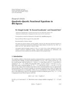
Figure 3: An image example for three image classes. (a) Synthetic image (chart), (b) mammography, and (c) remote sensing SST AfrNW 5
image.

function is
f0 u1 = E l1 [2n + 1] − pT l1 [2n]
1

2

= E l0 [2n + 1]+ l1 [2n + 1] − pT l0 [2n]+ l1 [2n]
1

2

.

(43)
The prediction filter length determines the number of
even samples l1 [2i] employed by the prediction. Employing

the prediction filter taps
pT
1

= · · · p1,i−1 p1,i p1,i+1 · · ·

(44)

the objective function is set in a summation form as
⎡

f0 u1 = E ⎣ wlT[2n+1] x + uT AT [2n+1] x
1 l0
0
2

−
i

p1,i wlT[2(n+i)] x
0

−
i

p1,i uT AT [2(n+i)] x
1 l0

⎤
⎦.

(45)
The algebraic manipulation to attain the solution is similar to the previous case. The optimal update filter is expressed
as
T

u1 = AT R A − 2A p + A p RA p

−1

A − Ap

T

(46)
×R w p − wl0 [2n+1] ,

being the notation
A = Al0 [2n+1] ,
wp =
Ap =

i

i

p1,i wl0 [2(n+i)] ,
p1,i Al0 [2(n+i)] .

(47)

The final expression (46) is similar to the filter (40) obtained in the previous design. However, the optimal filter
emerging from this design differs from the previous one even
in the simple case that has two taps and the prediction is
p1 = (1/2 1/2)T . For larger supports, the difference is more
remarkable. These facts are analyzed in the experiments section.
7.
7.1.

EXPERIMENTS AND RESULTS
Interpolation methods results

The first part of this section is devoted to a more qualitative
assessment of the proposed interpolation methods. A practical reason impels to a nonexhaustive experimental setting.
The proposed quadratic interpolation formulation is very
rich and offers many different variants. The number of experiments to test all the possible variants is huge. The following points show such a variability and explain the basic
setting for the qualitative assessment. Experiments are done
for several image classes: natural, textured images, synthetic,
biomedical (mammography), and remote sensing (sea surface temperature, SST) images. Figure 3 shows an example
image from our database for the synthetic, mammography,
and SST image classes.
(1) As stated, the formulation accepts local and global
settings. Global means that the same quadratic class is selected for the whole image. In this case, the image model
should be chosen. For the local adaptive interpolation, the
local patches size and support have to be selected. In the
experiments below, the choice is 4 × 4 and 8 × 8, respectively. Furthermore, an initial interpolation is required. Different choices exist to this goal, the bicubic interpolation being the preferred one. Finally, the patches may be extracted
from other similar images or images from the same class.
(2) The interpolation method output may be re-introduced in the algorithm as an initial interpolation. The number of iterations may affect the final result and it should be
determined. The experiments below do not iterate if nothing

8

EURASIP Journal on Image and Video Processing

else is stated. Usually, one or two iterations improve the initial results, but in the subsequent iterations, the performance
tends to decrease.
(3) Five interpolation methods are highlighted in the previous sections, each of which may differently behave on each
image class.
(4) In addition, some of the methods are parameterdependant. The signal regularized and the energy penalizing
approaches balance two different objective functions according to a parameter (defined as γ and δ, resp.,) that has to be
tuned. The weighting objective matrix W in (16) should be
defined by the application or the image at hand. The distance
weighting depends on the image type, for example, a textured
image with a repeated pattern requires different weights than
a highly nonstationary image.
Clearly, the casuistry is important, but a general trend
may be drawn. The interpolation given by (7) has a better
global behavior than the others; it outperforms the other
methods and it reduces the 5/3 wavelet detail signal energy
from 5% to 20% for natural, synthetic, and SST images. The
results are poorer for the mammography and the texture images.
The weighted objective interpolation (16) attains very
similar results to (7), being better in some cases. For instance,
the interpolation error energy is around 3% smaller for the
texture image set.
The signal bound constraint (10) may be useful for images with a considerable amount of high-frequency content,
as the synthetic and SST classes. Some interpolation coefficients outside the bounds appear for this kind of images,
and thus, the method rectifies them. However, there is no error energy reduction and certainly a computational cost increases with respect to (7).
The signal regularized solution (22) performs very well

with small values of δ that give a lower weight to the regularizing factor with respect to the c vector l2 -norm objective. Interestingly, in the 1D case and with a difference matrix D relating all the neighboring samples, the objective factor Dx 2
coincides with xT R−1 x R being the autocorrelation matrix
of a first-order autoregressive process with the autoregressive
parameter ρ → 1. Therefore, the signal regularized method
may be seen as an interpolation mixing local signal knowledge with an image model.
Finally, it seems that the inclusion of the energy penalizing factor in the formulation is not useful for the image sets
because it damages the final result. The interest resides in its
relation with the signal regularized solution and for low values of γ. Maybe, this factor could be considered for highly
varying images in order to avoid the apparition of extreme
values.
The interpolation methods are further assessed with the
ensuing experiment. The bicubic interpolation is the benchmark and the comparison criterion is the PSNR, defined as
PSNR = 10 log10

2552
.
MSE

(48)

Table 1 shows some results concerning images with 512 × 512
pixels. Images are downsampled by a factor of 2. Each pixel is

the average of four highdensity pixels before the downsampling. Then, images are interpolated using different methods
and number of iterations. The setting resembles the inner
product used in the lifting application. It may be observed
in the table that the performance in terms of PSNR is better than the bicubic interpolation up to 2 dB. In addition of
the PSNR performance, it was shown in [7] that the resulting signals from the solution (7) are less blurry and sharper
around the existing edges. The related global interpolation
solution (9) is employed in the next section to test the ULS

performance.
7.2.

Lifting steps: optimality considerations

The formulation derived for the lifting filters may be employed as a tool to analyze existing filters optimality. The provided basis example is the 5/3 wavelet, but the same approach
is possible for any wavelet filter factorized into lifting steps.
An estimation or a model of the autocorrelation matrix
R is required in the global optimization approaches. In the
following experiments, images are assumed to be an autoregressive process of first-order (AR-1) or second-order (AR2). The autocorrelation matrix depends on the autoregressive
parameters. In the AR-1 case, R is completely determined by
parameter ρ, while in the AR-2 case, R is determined by the
second-order parameters a1 and a2 .
The optimality of the 5/3 update is studied according to
the AR image model. For fair comparison, the proposed ULS
employ two neighbors as the 5/3 ULS. Therefore, in practice
the application simply reduces to propose a coefficient different from 1/4 for the update filter (since it is symmetric). The
proposals attain noticeable improvements even in this simple
case.
Assuming an AR-1 process, the three linear ULS lead
to optimal filter coefficients depending on ρ as depicted in
Figure 4. The second and the third designs lead to similar coefficients. Meanwhile, the ULS coefficient arising from the
first design is smaller for all the intervals. Asymptotically
(ρ → 1), the second ULS design output doubles the coefficients of first and third ones. The update filter coefficients
are considerably below the 1/4 reference for the three designs and the usual ρ found in practice (which tends to be
near 1). This fact agrees with the common observation that
in some cases the ULS omission increases the compression
performance and that the ULS is generally included in the
decomposition process because of the multiresolution properties improvement. The issue of the ULS employment can
be approached from the perspective given by the proposed

linear ULS designs: the ULS is useful, but the correct choice
is an update coefficient quite smaller than 1/4 (as the three
ULS indicate for the usual ρ values).]
The optimal ULS for each of the three designs are also
derived assuming a second-order autoregressive model. For a
subset of the AR-2 parameters, the resulting optimal update
coefficients coincide with 1/4, but not for other possible values. Figure 5 highlights this fact for the second ULS design.
The figure relates the optimal update coefficient according
to the given criterion with respect to the AR-2 parameters.


J. Sol´ and P. Salembier
e

9

Table 1: Interpolation PSNR from the averaged and downsampled images using the bicubic, the initial quadratic interpolation (column
noted by A), and the distance weighted objective (B) with 1 and 2 iterations, and the regularized signal objective (C) with 1 iteration.
PSNR (dB)
Baboon
Barbara
Cheryl
Farm
Girl
Lena
Peppers

Bicubic
22.356
24.296

32.736
20.539
31.693
30.606
29.875

A-1 it.
23.810
25.653
34.161
22.265
33.232
32.107
31.105

A-2 it.
23.695
25.741
34.819
22.490
34.034
33.058
31.573

0.4

B-1 it.
23.717
25.610
34.091

22.176
33.147
32.049
31.149

C-1 it.
23.595
25.831
33.620
21.963
32.762
31.583
30.775
0.5

−0.8
−0.6

0.3

−0.4

0.25

−0.2

a2

0.35
Update filter coefficient

B-2 it.
23.745
25.753
34.759
22.486
33.936
32.960
31.648

0.2

0.25

0.1

0
0.05

0.2

0.15

0.4
0.1
0.05
0

0.01

0.6
0.8
0

0.2

0.4

0.6

0.8

0.5

1

AR-1 parameter
First ULS design
Second ULS design
Third ULS design

Figure 4: Update filter as function of the AR-1 parameter for the
three ULS designs. The update is a two-tap symmetrical filter and
so, only one coefficient is depicted. The first considered prediction
is the (1/2 1/2).

Six level sets of the update coefficient are depicted as a function of a1 and a2 . From the figure, it is concluded that 1/4 is
far from being optimal in the sense of (40) for many possible
image AR-2 parameters. To position a practical reference, the
three circles in Figure 5 depict the mean AR-2 parameters of

the synthetic, mammography, and SST image classes.
An experiment with synthetic data is done in order
to check the proposal performance for the assumed image
model. An AR-1 process containing 512 samples is decomposed into three resolution levels using the 5/3 wavelet prediction followed by the 5/3 update or one of the three ULS.
These four transforms are compared by computing the gradient l2 -norm of l(1) and the h(2) signal mean energy, which
1
1
are the second and third ULS objective functions. Figure 6
shows the mean results for 1000 trials. The relative gradient
and energy of the three ULS with respect to the 5/3 wavelet
are depicted.
Second and third designs are almost equal and outperform 5/3 in terms of energy and gradient for all ρ except for

1
a1

1.5

2

0

Figure 5: Six level-sets of a function of the update coefficient with
respect to the AR-2 parameters. The function is the absolute value
of the update coefficient minus 1/4. Thus, the resulting filter is very
similar to the 5/3 in the dark areas and different in the light areas. The circles depict the mean AR-2 parameters for the synthetic,
mammography, and SST image classes.

ρ 0.27; value for which the three design coefficients coincide. The first design shows worse performances, in particular for the case of small ρ. However, this design has more flexibility and may incorporate additional knowledge that leads
to a better image model.

7.3.

Coding results

This section applies the lifting filters to image coding. The 1D
filters are applied in a separable way.
7.3.1. Optimal ULS for image classes
The AR-1 parameter is estimated for three image classes.
Therefore, the model is useful for a whole corpus of images
instead of being local. Synthetic, mammography, and SST
images are used. Each corpus contains 15 images. The correlation matrix is determined by the AR-1 parameter, and
it is plugged into (36) in order to obtain an update filter


10

EURASIP Journal on Image and Video Processing
1.05
Energy high pass band (relative to LeGall 5/3)

Gradient l2 -norm (relative to LeGall 5/3)

1.08
1.06
1.04
1.02
1
0.98
0.96

0

0.2

0.4

0.6

0.8

1

1

0

0.2

0.4
0.6
AR-1 parameter

AR-1 parameter
First ULS design
Second ULS design
Third ULS design

0.8

1

First ULS design
Second ULS design
Third ULS design

(a)

(b)

Figure 6: (a) Relative gradient of l1 for the optimal ULS with respect to the 5/3 wavelet, and (b) relative energy of h(2) for the optimal ULS
1
with respect to the 5/3.

Table 2: Compression results with JPEG2000 using the standard
5/3 wavelet and the proposed optimal update with the AR-1 model
for the synthetic, mammography, and SST image classes. Results are
in bpp.
Rate (bpp)
Synthetic
SST
Mammography

5/3 wavelet
3.832
3.252
2.349

AR-1 model
3.508
3.123

2.358

used for all the images in a class. Image compression is performed with a four-resolution level decomposition within
the JPEG2000 coder environment. Numerical results appear
in Table 2 compared to the 5/3 wavelet. The proposal compression results improve those of the 5/3 for the synthetic and
SST image classes, but results slightly worsen for the mammography class. The latter case is analyzed in the next experiment.
7.3.2. A refinement for mammography
The optimal ULS results are worse for the mammography
image class with respect to the 5/3 wavelet. The reason may
be found in the structure of this kind of images. Clearly,
there are two differentiated regions: a homogenous dark one
containing the background and a light heterogeneous foreground. Background pixels are found at the smaller gray values, typically less than 50. Background and foreground have
distinct autocorrelation and AR parameters. The mean of
both AR parameters is not optimal for any of the two regions.
A more accurate approach for this class should contemplate

an AR model or derive an autocorrelation matrix for each of
the two regions separately.
The AR-1 and AR-2 parameters are estimated for each
region. The second and third ULS are derived using both
models. All the approaches lead to similar update coefficients, which are close to dyadic coefficients: 1/8 for the background and 1/32 for the foreground. Therefore, the background and foreground filters are set to ub = (1/8 1/8)T and
u f = (1/32 1/32)T , respectively.
Once the coefficients are determined, images are decomposed with a space-varying ULS that depends on the next
approximation coefficient value. If this coefficient is greater
than the threshold T, it means that the region is foreground
and the u f filter is employed. Otherwise, the region is considered to be background and the optimal filter for the background ub is used:
⎧
⎪
⎨l0 [n] + uT h1 [n],

if l0 [n + 1] > T,

⎩l0 [n] + uT h1 [n],

otherwise.

l1 [n] = ⎪

f

b

(49)

The decoder has to take into account this coding modification in order to be synchronized with respect to the coder
and to decide the filter according to the same data.
Image compression is again performed with a fourresolution level decomposition within the JPEG2000 coder
environment. The selected threshold is T = 50. The mean
results for the 15 mammographies decrease from 2.358 bpp
to 2.336 bpp.


J. Sol´ and P. Salembier
e
8.

CONCLUSIONS

This paper develops a linear framework employed to derive
new lifting steps. The starting point is a quadratic interpolation method from which several alternatives are given. The

conclusion regarding the proposed methods is that their performance in terms of PSNR is around 1.5 dB better than the
bicubic interpolation when the image being interpolated has
been lowpass filtered before the downsampling. However, the
final result depends on the appropriate choice of the interpolation method and its parameters to the image at hand.
In a natural way, the initial interpolation formulation is
used for the design of lifting steps by adding an extra set of
linear equality constraints in the formulation due to the inner product of the discrete wavelet transform coefficients.
This permits the design of PLS minimizing the detail signal energy and the design of ULS with approximation signal
gradient criteria. Indeed, the optimal interpolation obtained
with any of the precedent methods may be applied to create
new PLS and ULS.
The framework is also employed for an optimality analysis of the 5/3 wavelet according to the established criteria.
The main conclusion is that there are image classes for which
this commonly used wavelet is not optimal. The compression results within the JPEG2000 environment confirm this
observation. Also in this case, a correct choice of the image
model and parameters is required to obtain the best results.
Finally, the developed lifting framework seems to be very
flexible. A variety of other experiments may be envisaged as a
future work. Different image models could be used to derive
first and second PLS, ULS, space-varying and adaptive ULS,
lifting steps on quincunx grids, and so forth. Also, it would
be interesting to establish the strict relation between the interpolation performance and the performance of the lifting
steps derived using this interpolation.
ACKNOWLEDGMENT
This work is partially financed by TEC2004-01914 Project of
the Spanish Research Program.
REFERENCES
[1] W. Sweldens, “The lifting scheme: a custom-design construction of biorthogonal wavelets,” Applied and Computational
Harmonic Analysis, vol. 3, no. 2, pp. 186–200, 1996.
[2] A. Gouze, M. Antonini, M. Barlaud, and B. Macq, “Design of

signal-adapted multidimensional lifting scheme for lossy coding,” IEEE Transactions on Image Processing, vol. 13, no. 12, pp.
1589–1603, 2004.
[3] H. Li, G. Liu, and Z. Zhang, “Optimization of integer wavelet
transforms based on difference correlation structures,” IEEE
Transactions on Image Processing, vol. 14, no. 11, pp. 1831–
1847, 2005.
[4] J. Hattay, A. Benazza-Benyahia, and J.-C. Pesquet, “Adaptive
lifting for multicomponent image coding through quadtree
partitioning,” in Proceedings of IEEE International Conference
on Acoustics, Speech and Signal Processing (ICASSP ’05), vol. 2,
pp. 213–216, Philadelphia, Pa, USA, March 2005.

11
[5] J. Sol´ and P. Salembier, “A common formulation for interpoe
lation, prediction, and update lifting design,” in Proceedings of
IEEE International Conference on Acoustics, Speech and Signal
Processing (ICASSP ’06), vol. 2, pp. 13–16, Toulouse, France,
May 2006.
[6] J. Sol´ and P. Salembier, “Adaptive quadratic interpolation
e
methods for lifting steps construction,” in Proceedings of the
6th IEEE International Symposium on Signal Processing and Information Technology (ISSPIT ’06), pp. 691–696, Vancouver,
Canada, August 2006.
[7] D. D. Muresan and T. W. Parks, “Adaptively Quadratic (AQua)
image interpolation,” IEEE Transactions on Image Processing,
vol. 13, no. 5, pp. 690–698, 2004.
[8] S. Boyd and L. Vandenberghe, Convex Optimization, Cambridge University Press, Cambridge, UK, 2004.
[9] “ISO/IEC 15444-1: JPEG 2000 image coding system,”
ISO/IEC, 2000.
[10] A. T. Deever and S. S. Hemami, “Lossless image compression

with projection-based and adaptive reversible integer wavelet
transforms,” IEEE Transactions on Image Processing, vol. 12,
no. 5, pp. 489–499, 2003.