Báo cáo hóa học: " Research Article Real-Time 3D Face Acquisition Using Reconfigurable Hybrid Architecture" pptx

Hindawi Publishing Corporation
EURASIP Journal on Image and Video Processing
Volume 2007, Article ID 81387, 8 pages
doi:10.1155/2007/81387
Research Article
Real-Time 3D Face Acquisition Using Reconfigurable
Hybrid Architecture
Johel Mit
´
eran, Jean-Philippe Zimmer, Michel Paindavoine, and Julien Dubois
Le2i Laboratory, University of Burgundy, BP 47870, 21078 DIJON Cedex, France
Received 2 May 2006; Revised 22 November 2006; Accepted 12 December 2006
Recommended by Joern Ostermann
Acquiring 3D data of human face is a general problem which can be applied in face recognition, virtual realit y, and many other ap-
plications. It can be solved using stereovision. This technique consists in acquiring data in three dimensions from two cameras. The
aim is to implement an algorithmic chain which makes it possible to obtain a three-dimensional space from two two-dimensional
spaces: two images coming from the two cameras. Several implementations have already been considered. We propose a new sim-
ple real-time implementation based on a hybrid architecture (FPGA-DSP), allowing to consider an embedded and reconfigurable
processing. Then we show our method which provides depth map of face, dense and reliable, and which can be implemented
on an embedded architecture. A various architecture study led us to a judicious choice allowing to obtain the desired result. The
real-time data processing is implemented in an embedded architecture. We obtain a dense face disparity map, precise enough for
considered applications (multimedia, vir tual worlds, biometrics) and using a reliable method.
Copyright © 2007 Johel Mit
´
eran et al. This is an open access article distributed under the Creative Commons Attribution License,
which permits unrestricted use, distribution, and reproduction in any medium, provided the original work is properly cited.
1. INTRODUCTION
We present in this paper a comparison of numerous methods
allowing obtaining a dense depth map of human face, and the
real-time implementation of the chosen method. Acquiring
3D data of human face is a general problem which can be

applied in face recognition [1–3]. In this particular case, the
knowledge of depth map can be used for example as a classi-
fication feature. It can be seen as an improvement of classical
methodsuchaseigenfaces[4]. The stereovision technique we
used is well known and consists in acquiring data in three di-
mensions from two cameras. The key problem in stereo is
how to find the corresponding points in the left and in the
right image [5] (correspondence problem). Many research
activities are currently dealing with stereovision, using differ-
ent approaches to solve the correspondence problem. Since
our main application is face recognition, we studied differ-
ent methods adapted to this problem. Moreover, our appli-
cationshavetobecompletedinreal-time(10image/s).Gen-
eral purpose computers are not fast enough to meet these re-
quirements because of the algorithmic complexity of stereo-
vision techniques. We studied the implementation using hy-
brid approach. Although various implementations have al-
ready been c onsidered [6, 7], we propose a simple real-time
implementation, including a regularization step, based on a
multiprocessor approach (FPGA-DSP) allowing to consider
an embedded and reconfigurable processing. Faugeras et al.
[6] proposed a multi-FPGA (23 Xilinx 3090) architecture
which is too complex for an embedded application. Ohm and
Izquierdo [7] proposed a stereo algorithm where dense map
is obtained using bilinear interpolation from global disparity
estimation. However, this approach used for face localization
is not enough precise for face recognition problem. In [8],
Porr et al. used the Gabor-based method implemented in a
software and hardware system. The board is virtex-based as
ours, but does not allow embedded post processing as we do

in the DSP from Texas Instrument. We present in the first
part of the paper the study of the whole necessary process-
ing, while reviewing and comparing various employed meth-
ods. In the second part, we present the implementation on an
embedded architecture of our method which provides depth
map of face, dense and reliable.
2. METHOD
2.1. Stereodata processing flow
The main goal of this whole processing is to match corre-
sponding points between two images. The distance or dis-
parity between these homologous points is then calculated.
2 EURASIP Journal on Image and Video Processing
P
C
1
C
0
C
2
F
f
1
f
2
p
1
p
2
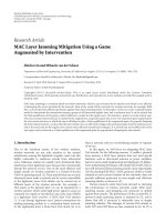
Figure 1: Retina disparity.
This value is proportional to the depth, thus codes the third

dimension (Figure 1).
The retina disparity D is defined as follows:
D
= E

f
1
, p
1

− E

f
2
, p
2

,(1)
where E(x, y) is the Euclidian distance between x and y.
This value is proportional to the depth difference be-
tween P and F.
The processing flow is composed of two main parts. The
first requires mainly geometrical criteria and modeling, the
second uses signal processing knowledge.
The first part is the camera calibration, either for each
one in 3D space (strong calibration) or relatively between
them (weak calibration and epipolar geometry). To this stage
can be a dded a rectification image processing. This rectifica-
tion allows to match the image lines of the stereo pair, and
thus to work in only one dimension [5].

The second part consists in the homologous points
matching. Various methods were developed to constitute
dense depth maps. Two papers [9, 10 ]presentalargereview
of these techniques. Since the goal of this paper is mainly
to present the hardware implementation of our solution, we
will only recall the principle of the 3 methods we compared,
the results of this comparison which will justify our final
choice.
2.2. Principal methods of dense depth maps
constitution
Several methods have been studied and give interesting re-
sults. We can classify them in three principal parts: the meth-
ods based on partial differential equation (PDE) [11], on lo-
cal phase [12], and on crosscorrelation [13].
2.2.1. Partial differential equations
This method is based on the minimization of an energy cri-
terion by solving a diffusion equation. Various implementa-
tions were given. One of them provides the depth by reso-
lution of the discrete Euler-Lagrange equation [14]. A judi-
cious choice of the regularization function allows preserving
discontinuities [11]. A multiresolution result is obtained by
iteratively searching for the solution. In order to obtain ef-
ficient solutions, it can be here interesting to introduce the
epipolar constraint.
The methods based on PDE allow obtaining dense depth
maps and a very good precision on the results. Unfortunately,
these processing require too significant computing times and
cannot, yet, be considered on a simple embedded architec-
ture. Therefore, we did not include this method in our com-
parison.

2.2.2. Crosscorrelation
This classical method is based on homologous points match-
ing by search of the minimum of a criterion by crosscorre-
lation in shifting local windows [13]. The most usual crite-
ria used are the crosscorrelation or the square difference (or
the difference absolute value) of the pixel intensities between
each image of the stereopair. This method can be improved,
in order to make it less sensitive to the differences between
the average gray level of the two images, by centering and/or
by a local normalization. Moreover, the criterion is applied
in a local window surrounding the tested pixels. The crite-
rion C
x,y
is then computed as follows:
C
x,y
=

−l≤i≤l; −h≤j≤h

I
1
(x + i, y + j) − I
1
(x, y)

−

I
2

(x + i, y + j) − I
2
(x, y)

2
,
(2)
where I
1
(x, y) is the pixel luminance of left image, I
2
(x, y)is
the pixel luminance of right image, and h and l are, respec-
tively, the height and length of the local window centred in
(x, y).
I
1
(x, y)andI
2
(x, y) are the mean of luminance com-
puted in these local windows.
The method of shifting window processing requires a
range of limited disparities [d
1
, d
2
]. The criterion is then cal-
culated for each disparity. The maximum criterion gives the
required disparity. If the maximum is obtained for d
1

or d
2
,
an error value is affected to D (Figure 2).
This processing is carried out effectively in one dimen-
sion and thus requires either to know the epipolar constraint,
or to work on rectified images. A double processing Left Im-
age/Right Image then Right Image/Left Image, followed by a
validation step, makes it possible to remove wrong matching.
A multiscale approach can also be considered, allowing
an extension of the range of the required disparities and a
validation at various scales in order to obtain better results
on poorly textured patterns. Improvements were planned
in order to obtain better answers in the presence of local
discontinuities. Fusiello et al. [15] uses several local win-
dows around the pixel. De vernay [5] uses a local window in
form of parallelogram, and deforms it to obtain a minimum
Johel Mit
´
eran et al. 3
H
L
y
0
l
h
x
0
x
0

+ d
1
x
0
+ d
0
x
0
+ d
2
Left image Right image
C
x,y
(d)
C
max
d
1
d
0
d
2
d
Figure 2: Crosscorrelation-based matching.
criterion. These two methods allow introducing local dispar-
ity gradients.
In our case, we improve the correlation results during a
regularization step composed by a parabolic approximation
of the correlation (allowing subpixel interpolation) and a
morphological filtering which allows removing artifacts. The

parabolic interpolation is given by
d(x, y)
= d
0
(x, y)+
1
2
C
x,y

d
0
+1

−
C
x,y

d
0
− 1

2C
max
− C
x,y

d
0
+1


− C
x,y

d
0
− 1

.
(3)
2.2.3. Local phase
The algorithm uses the image local phases estimates for
the disparity determination [13]. Phase differences, phase
derivative, and local frequencies are calculated by filtering the
stereocouple with Gabor filters, as follows:
I
1G
(x) = I
1
(x) ∗ G(x, σ, ω),
I
2G
(x) = I
2
(x) ∗ G(x, σ, ω),
(4)
with the Gabor kernel defined as
G(x, σ, ω)
=
1

√
2πσ
e
−x
2
/(2πα)
2
,(5)
and the local phases are defined as
Φ
1
(x) = arctan

Im

I
1G
(x)

Re

I
1G
(x)


,
Φ
2
(x) = arctan


Im

I
2G
(x)

Re

I
2G
(x)


.
(6)
The disparity d is calculated from estimates of local phases in
images I
1
and I
2
using
d
ω
(x) =

Φ
1
(x) − Φ
2

(x)

ω
,(7)
where ω is the average local spatial frequency.
The processing allows then to deduce local disparities
[16]. The frequency scale limitations and the phase wrapping
problem impose to limit the disparity. To obtain a higher
range of disparity, it is necessary to resort to a coarse-fine
strategy in which the results for each s cale are extended and
used on the following scale, thus making it possible to in-
crease the limits of disparity variations [17]. A regularization
step introduces a smoothing constraint for each scale by fit-
ting the results to a spline surface. These methods are related
to recent discoveries in physiology of three-dimensional per-
ception [18, 19].
Another method based on local phase determination uses
complex wavelets [20]. Through its robustness against light-
ing variation and additive noise, this method extends the
properties of the Gabor wavelets to the differenc es in lumi-
nosity variation and to additive noise. But especially this op-
erator provides shift invariance and a good directional selec-
tivity. These conditions are essential to obtain disparity. The
disparity computation is carried out by a difference between
the detail coefficients of the left and right images. An adjust-
ment by a least square method gives an optimal disparity, de-
pending on the phase, and insensitive to intensit y changes
[21]. The epipolar constraint can be added effectively for a
better determination of homologous points [22].
2.3. Methods comparison in the case of

face acquisition
In order to choose a good compromise between performan-
ces and speed processing, we measured the quadratic error
between a model of face and the stereo acquisition.
The error is defined as
Q
=
1
LH
H

y=1
L

x=1


O(x, y) − S(x, y)


2
,(8)
where O(x, y) represents the depth map obtained using our
algorithms and S(x, y) is the model depth map, obtained us-
ing a 3D laser-based scanner.
The face used for the comparison is depicted in Figure 3.
We studied the error depending on the focal length used
during acquisition. We showed in [23] that the optimum
choice for the stereo device depends on the focal length and
that this optimum can be chosen around f

= 30 mm for a
standard CCD-based camera.
4 EURASIP Journal on Image and Video Processing
Rectified images of test face
Reference depth map
Figure 3: Reference face.
Figure 4: Left and right acquired images, depth maps without and
with post processing.
The maps obtained by crosscorrelation can b e very cor-
rect, under certain conditions of illumination. For our part,
we obtained good dense depth map by projecting a random
texture on the face. Nevertheless, a post processing is re-
quired in order to effectively improve the existing discon-
tinuities. This processing can be filled by a morphological
opening and closing, followed by a Gaussian blur to smooth
small discontinuities correctly. Figure 4 shows the results ob-
tained with and without filtering.
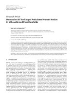
The images obtained using the three compared meth-
ods are depicted on Figure 5, and the corresponding error
is depicted on Figure 6. It is clear that, although the Gabor
wavelets-based method seems to be the best choice, the per-
formances are very close from each other when focal length is
near f
= 30 mm. This justifies our final choice of implemen-
tation, based on the crosscorrelation algorithm, for which the
(I) f = 28.5 mm (II) f = 32 mm (III) f = 35.3mm
(a) Results using crosscorrelation
(I) f = 28.5 mm (II) f = 32 mm (III) f = 35.3mm
(b) Results using filtered crosscorrelation
(I) f = 28.5 mm (II) f = 32 mm (III) f = 35.3mm

(c) Correlation using multiple windows
(I) f = 28.5 mm (II) f = 32 mm (III) f = 35.3mm
(d) Results using Gabor wavelets
Figure 5: Depth maps.
Johel Mit
´
eran et al. 5
0.35
0.4
0.45
0.5
0.55
0.6
0.65
0.7
0.75
0.8
RMSE
17 19 21 23 25 27 29 31 33 35
Focal distance (mm)
Crosscorrelation
Gabor
Multiple window
Figure 6: Error comparison.
Rectification Local centering
Rectification Local centering
Matching Filtering
Depth map
Figure 7: Computed chain implemented to obtain dense depth
map.

hardware implement cost will be clearly lower than in the Ga-
bor wavelets case.
3. PROCESSING, RESULTS, AND IMPLEMENTATION
Since we obtained using software simulation dense and pre-
cise depth maps, we implemented the crosscorrelation by
shifting windows algorithm. The whole algorithm is dis-
tributed as shown in Algorithm 1, and is depicted in Figure 7.
In the first stage after image acquisition, we carry out an
image rectification. This processing is computed through a
weak calibration and the fundamental matrix determination
[24]. The rectification matrices are obtained by an original
computation, based on a projective method [25], by calcu-
lating the homogr aphy of four points of each image plan.
We carry out then a local centering of the images thus al-
lowing reducing the problems involved in the average inten-
sity differences between the two views. Data normalization
does not produce more reliable results.
The following step is the two images matching, on a de-
fined disparity range. This calculation is applied by a cross-
correlation by shifting windows. The used criterion is the dif-
ference absolute value sum (DAS). We sort then the values to
seek their minimum.
(1) Acquisition of left and right images.
(2) Rectification of left and right images.
(3) Local centering of left and right images.
(4) Matching using crosscorrelation.
(a) Crosscorrelation computation (2).
(b) Disparity computation, using the search of maxi-
mum value of crosscorrelation and subpixel interpo-
lation.

(5) Filtering of the depth map.
Algorithm 1
Table 1: Operation required.
Number of operations
Rectification 2 × 4 × L × H
Local centering
2 × 21 × L × H
Matching-crosscorrelation
21 × L × H × D
Matching-max determination
(2 × D
r
+3)× L × H
Tota l
(23 × D
r
+ 53) × L × H
We evaluated the number of operations to be performed
in order to map the algorithm on an embedded architecture.
In order to realize a f ast processing of the local centering
and the crosscorrelation, we use an optimized computing al-
gorithm described hereafter. Because of this algorithm, the
number of operations we carry out is no more proportional
to the crosscorrelation window size.
So, we have to compute the following values:
C
r
(x) = C
r
(x − 1) − C(x − l)+C( x),

C
rc
(x) = C
rc
(x − 1) + C
r
(x) − C
r
(x − hL),
(9)
where, C
r
and C
rc
are intermediate values, x represents the
current computed value index and x
− 1 the previous index,
h and l are the height and the width of the crosscorrelation
window and L is the image width. The C
r
and C
rc
values are
the results of a previous computing of the crosscorrelation.
C
r
is the value computed in an h pixels row wide, and C
rc
is
the value computed in an h

× l pixels window. These values
must be computed in real-time in order not to break the data
flow.
The C
r
and C
rc
values are 16 bits coded and must be
stored into arrays. The capacities of these needed arrays are
for C
rc
, the line width, and for C
r
, the line width multiplied
by the crosscorrelation window height. This processing is
therefore a more important consumer of memory space than
a crosscorrelation classical computing. Moreover, memories
must be managed with a lot of consideration in order not to
break the data flow of the whole processing.
We examine in Table 1 the number of operations we
need to realize the different processing. The operations we
use are elementary and include simple arithmetic operations
6 EURASIP Journal on Image and Video Processing
Table 2: Virtex devices.
Device
System
gates
CLB
array
Logic

cells
Block
RAM
bits
Block
RAM
number
XCV300 322970 32 × 48 6912 65536 16
XCV800 888439 56
× 84 21168 114688 28
(addition or subtraction), incrementations of values for the
loops and access memory operations.
In this table, H and L are the height and the width of the
image and D
r
the disparity range value. After some studies of
this algorithm working on human faces [23], we determined
the optimal values for the crosscorrelation window size and
the disparity range. We use a 256
×256 pixels image size, a 7×
6 pixels crosscorrelation window size and 20 for the disparity
range. The number of operations we have to compute is then
equal to 33, 62 Mops per trame, or 840 Mops per second for
a 25-image-per-second video standard.
In order to optimize the implementation of the steps 1, 2,
3, and 4a in Algorithm 1 using parallel computing, we choose
to use a reconfigurable logical device.
Theseprocessingsarecarriedouteffectively on the XIL-
INX FPGA Virtex. Virtex devices provide better performance
than previous generations of FPGA. Designs can achieve

synchronous system clock rates up to 200 MHz including
for Inputs-Outputs. Virtex devices feature a flexible regu-
lar architecture that comprises an array of configurable logic
blocks (CLB) surrounded by programmable input/output
blocks (IOBs), all interconnected by a hierarchy of fast and
versatile routing resources. They incorporate also several
large blocks RAM memories. Each block RAM is a fully
synchronous dual-ported 4096-bit with independent control
signal for each port. The data widths of the two ports can
be configured independently. Thus, each block has 256 datas
of 16- bit capacity. Each memory blocks are organized in
columns. All Virtex devices contain two such columns, one
along each vertical edge. The Virtex XCV300 and XCV800
capacities are grouped together in Ta ble 2.
An original parallel implementation, described in the
next paragraph, allows a very fast calculation of the criteria
on all the disparity range.
These results are then given to a DSP which carries out
successively the following processing: a para bolic interpola-
tion to obtain wider disparity values; morphological filtering
made up of an opening then a closing to eliminate wrong
disparities while keeping depth map precision; a Gaussian
blurring filter finally to smooth the obtained results. These
processings are optimized on a C6x Texas Instrument DSP
which allows a fast data processing.
3.1. Description of the chosen architecture
The constraints imposed by the algorithmic sequence real-
time computing and the needed compactness to obtain
an embedded architecture lead us to choose a reconfig-
Frame Grabber

SBSRAM
SBSRAM
SBSRAM
SBSRAM
VPE
FPGA
Virtex Xilinx
FIFO
FIFO Global SRAM
PCI controller
DSP
TI C44
DSP
TI C67
SDRAM
Figure 8: Parts of the board architecture.
urable and multiprocessor FPGA-DSP set: the Mirotech
Arix Board. This board is designed in se veral indepen-
dent computing parts, with configurable links. External
links allow us to interface the board with a real-time
Frame Grabber (FG) and with a PC (through the PCI
bus). The computing parts are as follows (Figure 8): one
virtual processing element (VPE) consisting of a Xil-
inx Virtex FPGA (XCV300 or XCV800) with four 512ko
SBSRAM memory blocks; the second is composed of
one Texas Instrument TMS320C44 DSP with two 1Mo
SRAM memory blocks. This DSP interfaces two TIM
sites on which we can connect the third computing el-
ement. For this part, we choose one Texas Instrument
TMS320C67 DSP with an 8Mo SDRAM memory block.

These three parts are connected by configurable links that
allow direct memory access (DMA). Thus whole process-
ing can be done in pipeline, cascaded in several parts as
FG
⇒VPE⇒DSPC44⇒DSPC67⇒DSPC44⇒PCI.
This reconfigurable architecture allows us to quickly re-
alize and validate our algorithm-architecture suitability.
3.2. Matching implementation
The most important computation time is required by the
matching processing; so we made a particular effort to imple-
ment this part. To obtain real-time results, we use the opti-
mised crosscorrelation technique implemented using the in-
trinsic parallelism of FPGA.
This method, described in a previous section, allows an
important time gain by reusing intermediary computed re-
sults. Although a C language implementation of this algo-
rithm is relatively simple, its FPGA implementation presents
more problems. The main is memory management. Indeed,
this processing needs a lot of intermediary values, easily al-
located in C on a PC. Unfortunately, in order to respect the
real-time constraint, we have to reduce the memory access
and manage the best possible intermediary values and the
data flow. Three processing parts are implemented: the first
(Figure 9(a)) for the DAS parallel processing on the disparity
Johel Mit
´
eran et al. 7
V(2)
V(1)
V(2, 0) V(2, 1) V(2, N)

+
− + − + −
Sum Sum Sum
ABS ABS ABS
C( x,0) C(x,1) C(x, N)
V(1) and V(2)
from previous
processing on the
stereo pair
(a) DAS computing
C
r
(x, N)
C
r
(x, N)
FIFO7
Cpt > 7
Cpt
≥ 7ACC
+
−
+
Sum
C
rc
(x, N)
(b) Intermediate values computing
C
r

(x, N)
C
rc
(x, N)
−
+
Sum
F(N)
C
rc
(N)
(c) Final v alues computing
Figure 9: Matching implementation.
range; the second (Figure 9(b)), for the intermediary values
parallel computing, and the third (Figure 9(c)) for the final
computing. These two first parts hold, respectively, 9% and
6% slices of a Virtex300 FPGA.
For the parallel processing, we connect N times (N is be-
tween 0 and 19) the second part to all the outputs of the first
part. We obtain thus in parallel the whole criteria needed
to compute the disparity for one pixel. The C
rc
criteria are
stored in the Virtex memory blocks at the rate of one mem-
ory block per disparity. The C
r
criteria are alternately stored
into two SBSRAM blocks of the Arix bo ard. For each even
line, the writing is carried out into the first block and, for
the odd lines, into the second block. The two memory blocks

can then be used in paral lel. This allows processing the third
part, in which a reading of the C
rc
and C
r
criteria is carried
out, without any influence onto the two other parts.
The whole final criteria, named F(N), are then used for
the determination of the maximum disparity onto the dis-
parity range. The maximum disparity is determined, and we
keep, with this value, the previous and the following dispar-
ity values. These three values are then sent to the DSP (which
is well adapted to floating point processing) for a subpixel
determination of the disparity (a parabolic interpolation, ac-
cording (3)).
4. CONCLUSIONS AND PERSPECTIVES
We compared in the present paper various stereo matching
methods in order to study real-time 3D face acquisition.
We have shown that it is possible to implement a simple
crosscorrelation-based algorithm with good performances,
using post processing. A var ious architecture study led us
to a judicious choice allowing obtaining the desired result.
The real-time data processing is implemented on an embed-
ded architecture. We obtain a dense face disparity map, pre-
cise enough for considered applications (multimedia, virtual
worlds, biometrics) and using a reliable method. In particu-
lar, we plane to use the results as features for a face recogni-
tion software described in a previous article [26].
REFERENCES
[1] C. Beumier and M. Acheroy, “Automatic face verification from

3D and grey level clues,” in Proceedings of the 11th Portuguese
Conference on Pattern Recognition (RECPAD ’00), pp. 95–101,
Porto, Portugal, May 2000.
[2] T. S. Jebara and A. Pentland, “Parametrized structure from
motion for 3D adaptive feedback tracking of faces,” in Pro-
ceedings of the IEEE Computer Society Conference on Computer
Vision and Pattern Recognition (CVPR ’97), pp. 144–150, San
Juan, Puerto Rico, USA, June 1997.
[3] J.Y.Cartoux,Formes dans les images de profondeur. Application
`
a la reconnaissance et
`
a l’authentification de visages,Ph.D.the-
sis, Universit
´
e Blaise Pascal, Clermont-Ferrand Cedex, France,
1989.
[4] M. Turk and A. Pentland, “Eigenfaces for recognition,” Journal
of Cognitive Neuroscience, vol. 3, no. 1, pp. 71–86, 1991.
[5] F. Devernay, Vision st
´
er
´
eoscopique et propri
´
et
´
es diff
´
erentielles des

surfaces, Ph.D. thesis, Ecole Polytechnique, l’Institut National
de Recherche en Informatique et en Automatique, Chesnay
Cedex, France, 1997.
[6] O. Faugeras, B. Hotz, H. Mathieu, et al., “Real time corre-
lation based stereo: algorithm implementations and applica-
tions,” Tech. Rep. RR-2013, l’Institut National de Recherche
en Informatique et en Automatique, Chesnay Cedex, France,
1993.
[7] J R. Ohm and E. M. Izquierdo, “An object-based system for
stereoscopic viewpoint synthesis,” IEEE Transactions on Cir-
cuits and Systems for Video Technology, vol. 7, no. 5, pp. 801–
811, 1997.
[8] B. Porr, A. Cozzi, and F. W
¨
org
¨
otter, “How to “hear” visual
disparities: real-time stereoscopic spatial depth analysis using
temporal resonance,” Biological Cybernetic s,vol.78,no.5,pp.
329–336, 1998.
[9] A. Koschan, “What is new in computational stereo since 1989:
a sur vey of current stereo papers,” Technischer Bericht 93-22,
Technische Universite
¨
at Berlin, Berlin, Germany, 1993.
[10] U. R. Dhond and J. K. Aggarwal, “Structure from stereo—a
review,” IEEE Transactions on Systems, Man and Cybernetics,
vol. 19, no. 6, pp. 1489–1510, 1989.
[11] L. Alvarez, R. Deriche, J. Sanchez, and J. Weickert, “Dense dis-
parity map estimation respecting image discontinuities,” Tech.

Rep. 3874, l’Institut National de Recherche en Informatique et
en Automatique, Chesnay Cedex, France, 2000.
[12] M. R. M. Jenkin and A. D. Jepson, “Recovering local sur-
face structure through local phase difference measurements,”
CVGIP: Image Understanding, vol. 59, no. 1, pp. 72–93, 1994.
8 EURASIP Journal on Image and Video Processing
[13] P. Fua, “A parallel stereo algorithm that produces dense depth
maps and preserves image features,” Machine Vision and Ap-
plications, vol. 6, no. 1, pp. 35–49, 1993.
[14] R. Deriche and O. Faugeras, “Les EDP en traitement des im-
ages et vision par ordinateur,” Traitement du Signal, vol. 13,
no. 6, 1996.
[15] A. Fusiello, V. Roberto, and E. Trucco, “Efficient stereo with
multiple windowing,” in Proceedings of the IEEE Computer So-
ciety Conference on Computer Vision and Pattern Recognition
(CVPR ’97), pp. 858–863, San Juan, Puerto Rico, USA, June
1997.
[16] M. W. Maimone and S. A. Shafer, “Modeling foreshortening
in stereo vision using local spatial frequency,” in Proceedings of
the IEEE/RSJ International Conference on Intelligent Robots and
Systems (IROS ’95), vol. 1, pp. 519–524, Pittsburgh, Pa, USA,
August 1995.
[17] J. Hoey, “Stereo disparity from local image phase,” Tech. Rep.,
University of British Columbia, Vancouver, British Columbia,
Canada, June 1999.
[18] I. Ohzawa, G. C. DeAngelis, and R. D. Freeman, “The neural
coding of stereoscopic depth,” NeuroReport,vol.8,no.3,pp.
3–12, 1997.
[19] P. Churchland and T. Sejnowski, The Computational Brain,
MIT Press, Cambridge, Mass, USA, 1992.

[20] N. Kingsbury, “Image processing with complex wavelets,”
Philosophical Transactions of the Royal Society A: Mathematical,
Physical and Engineering Sciences, vol. 357, no. 1760, pp. 2543–
2560, 1999, on a discussion meeting on “wavelets: the key to
intermittent information?”, London, UK, February 1999.
[21] H. Pan and J. Magarey, “Phase-based bidirectional stereo in
coping with discontinuity and occlusion,” in Proceedings of In-
ternational Workshop on Image Analysis and Information Fu-
sion, pp. 239–250, Adelaide, South Australia, November 1997.
[22] J. Magarey, A. Dick, P. Brooks, G. N. Newsam, and A. van den
Hengel, “Incorporating the epipolar constraint into a mul-
tiresolution algorithm for stereo image matching,” in Proceed-
ings of the 17th IASTED International Conference on Applied
Informatics, pp. 600–603, Innsbruck, Austria, February 1999.
[23] J P. Zimmer, “Mod
´
elisation de visage en temps r
´
eel par
st
´
er
´
eovision,” Thesis, University of Burgundy, Dijon, France,
2000.
[24] Z. Zhang, “Determining the epipolar geometry and its un-
certainty: a review,” International Journal of Computer Vision,
vol. 27, no. 2, pp. 161–195, 1998.
[25] R. I. Hartley, “Theory and practice of projective rectification,”
International Journal of Computer Vision,vol.35,no.2,pp.

115–127, 1999.
[26] J P. Zimmer, J. Mit
´
eran, F. Yang, and M. Paindavoine, “Se-
curity software using neural networks,” in Proceedings of the
24th Annual Conference of the IEEE Industrial Electronic s Soci-
ety (IECON ’98), vol. 1, pp. 72–74, Aachen, Germany, August-
September 1998.