Báo cáo hóa học: " A Space/Fast-Time Adaptive Monopulse Technique" doc
Bạn đang xem bản rút gọn của tài liệu. Xem và tải ngay bản đầy đủ của tài liệu tại đây (870.29 KB, 11 trang )
Hindawi Publishing Corporation
EURASIP Journal on Applied Signal Processing
Volume 2006, Article ID 14510, Pages 1–11
DOI 10.1155/ASP/2006/14510
A Space/Fast-Time Adaptive Monopulse Technique
Yaron Seliktar,
1
Douglas B. Williams,
2
and E. Jeff Holder
3
1
Jerusalem College of Engineering, P.O. Box 3566, Jerusalem 91035, Israel
2
School of Electrical and Computer Engineering, Georgia Institute of Technology, Atlanta, GA 30332-0250, USA
3
Sensors and Electromagnetic Applications Laboratory, Georgia Tech Research Institute, 7220 Richardson Road, Smyrna,
GA 30080-1041, USA
Received 28 October 2004; Revised 29 May 2005; Accepted 14 June 2005
Mainbeam jamming poses a particularly difficult challenge for conventional monopulse ra dars. In such cases spatially adaptive
processing provides some interference suppression when the target and jammer are not exactly coaligned. However, as the target
angle approaches that of the jammer, mitigation performance is increasingly hampered and distortions are introduced into the
resulting beam pattern. Both of these factors limit the reliability of a spatially adaptive monopulse processor. The presence of co-
herent multipath in the form of terrain-scattered interference (TSI), although normally considered a nuisance, can be exploited
to suppress mainbeam jamming with space/fast-time processing. A method is presented offering space/fast-time monopulse pro-
cessing with distortionless spatial array patterns that can achieve improved angle estimation over spatially adaptive monopulse.
Performance results for the monopulse processor are obtained for mountaintop data containing a jammer and TSI, which demon-
strate a dramatic improvement in performance over conventional monopulse and spatially adaptive monopulse.
Copyright © 2006 Hindawi Publishing Corporation. All rights reserved.
1. INTRODUCTION
A tracking radar requires a high-precision angular measure-
ment of a target’s azimuth (or elevation) which is tradi-
tionally achieved using monopulse processing. Historically,
monopulse radars employed two separ ate feed horns on
a single antenna element in order to generate two receive
beams that were slightly offset in azimuth (or elevation) an-
gle. Sum and difference outputs were formed by summing
and subtracting the two beam outputs, respectively. The ratio
of difference to sum output voltages, called the error voltage,
was then used to determine the degree of correction neces-
sary to realign the beam axis w ith the target.
With the introduction of phased array technology, it be-
came unnecessary to employ special hardware for monopulse
processing, since the array itself can electronically form the
multiple beams needed. A typical conventional monopulse
processor for a phased array radar is obtained by appropri-
ately phasing the individual array channels to obtain sum
and difference outputs. The ratio of difference to sum out-
puts provides the measure by which the angle offset from the
beam axis (i.e., look direction) is determined. The updated
angle measurement is then used to recompute phases for the
channels so as to realign the beam axis with the target.
Mainbeam jamming occurs when the jammer signal is
directly impinging on the radar’s receive beam. Spatially
adaptive processing works well when target and jammer are
adequately separated in angle. However, as the separation di-
minishes until target and jammer both appear within the
mainbeam, performance degrades [1]. This degradation is
most severe when the target and jammer are coaligned and
the spatially adaptive processor is unable to achieve any can-
cellation at all. The problem of using a spatially adaptive pro-
cessor is further compounded in that its pattern can become
very distorted in the presence of mainbeam jamming.
In [2, 3] it is shown that the coherent multipath com-
monly referred to in the radar literature as terrain-scattered
interference (TSI) can be exploited to significantly improve
the mitigation of interference. The operation of this proces-
sor is based on the principle that the direct path broadband
jammer can be used to predict and, thus, cancel the delayed
jammer reflections from the ground (i.e., TSI) present in the
mainbeam. Conversely, TSI can be used to estimate and can-
cel the direct path jammer in the mainbeam [2, 4–6]. In the
latter case the TSI is in effect used to form a “reference beam”
of the jammer, through which the jammer is cancelled. The
effectiveness of adaptive TSI processing for mitigating both
TSI and mainbeam jamming motivates us to investigate ways
of incorporating it with monopulse processing.
Other authors have considered the development of adap-
tive monopulse techniques, especially for situations in which
there is mainbeam jamming or clutter. For example, the
author in [7] implements a minimum variance monopulse
2 EURASIP Journal on Applied Signal Processing
processor in the STAP domain to extract simultaneous
direction-of-arrival (DOA) and Doppler estimates, with im-
provement cited by use of reduced sidelobe response (in the
joint angle-Doppler domain) in suppressing clutter.
The monopulse concept is further generalized in [8]to
include arbitrary parameter estimation in the STAP domain
with partial preprocessing (e.g., subarray) and generalized
beamforming.
The approach proposed here contra sts with those men-
tioned as well as others in two respects:
(i) the added dimensionality of the problem is in the fast
time as opposed to slow time (classic STAP);
(ii) the added dimensionality is strictly employed in utiliz-
ing to advantage a nuisance interference, TSI, in im-
proving DOA estimation.
The proposed approach is not offered as a competing ap-
proach to existing STAP monopulse techniques, but rather,
as a treatment of the specific problem of angle estimation
when either TSI alone or mainbeam jamming together with
TSI corrupt the sampled returns. In such scenarios slow-time
STAP by itself is of limited benefit since the sparsely spaced
coherent samples offer little benefit in predicting and subse-
quently mitigating the direct path mainbeam jammer signal
from its scattered multipath. By the same token the proposed
approach depends on the presence of strong TSI in the re-
turns, without which the incorporation of fast-time taps is of
little or no benefit for mainbeam jammer cancellation.
2. TSI PROCESSING
A radar has to contend with many forms of interference, in-
cluding jamming, clutter (ground returns), and TSI. The lat-
ter is the most complicated form of interference, and by far
the most difficult to suppress. Just as the radar’s transmitted
signal reflects from the surrounding terrain to form a com-
posite clutter signal at the aperture, so, too, can the jammer
signal reflect from the surrounding terrain to form TSI.
Such interference may be intentional or a result of the
poor sidelobe behavior that is characteristic of noise jam-
mers. The delayed and scaled jammer reflections integrate
at the aperture to form the composite TSI signal. Multi-
path components may be received over a wide angular ex-
tent and at varying delays potentially leading to signifi-
cant spatio-temporal correlation at the array elements. This
characteristic of TSI motivates the use of adaptive space/fast-
time (SFT) processing as discussed below.
2.1. Space/fast-time processing
Considered here is a r adar system that transmits a single
pulse and samples the returns on an N-element uniform lin-
ear array.
1
It collects L temporal samples
2
from each element
1
Application to planar arrays is possible at the expense of increased dimen-
sionality.
2
In our notation, N denotes a scalar constant, n a spatial vector, and N a
space-time vector or matrix. The transpose of a matrix or vector quantity,
N,isdenotedbyN
T
. Similarly, Hermitian transpose is denoted by N
H
.
receiver, where each time sample corresponds to a range cell.
The temporal dimension of interest here is referred to as fast
time.
3
The collection of samples is represented by an N × L
data mat rix X with elements x(n, l). A spatial snapshot con-
sists of N elements of spatial data from the lth range cell (i.e.,
lth column of X):
x(l)
=
x(0, l) x(1, l) ··· x(N − 1, l)
T
. (1)
Similarly, a SFT snapshot, X(l), consists of T consecutive spa-
tial snapshots in descending order of time index stacked into
a vector (i.e., a stack of T consecutive columns of X in de-
scending order of time index),
X(l)
=
x
T
(l) x
T
(l − 1) ··· x
T
(l − T +1)
T
. (2)
The output of a fast-time processor, z(l), is a weighted sum of
the components of the SFT snapshot, X(l), at a given instant
of time (index), l:
z(l)
= W
H
X(l). (3)
Thus, the SFT processor is described by the NT
× 1weight
vector W.
The simplest type of processing that can be performed
on the data is nonadaptive spatial processing (i.e., where T
=
1), also known as conventional processing. In conventional
processing,
W
= v
ν
=
1 e
j2πν
··· e
j2πν
(N−1)
T
(4)
is a spatial steering vector defined at spatial frequency ν
=
(D/λ) sin(φ
), where φ
is the target’s look direction, D is the
interelement spacing of the array, and λ is the ra dar’s operat-
ing wavelength [3].
2.2. TSI mitigation
More so than with clutter and jamming, TSI lacks a consis-
tent and predictable structure. As such, in mitigating TSI, it
is necessary to employ adaptive processing. Adaptive pro-
cessing represents a more sophisticated class of processors
and typically requires solving for a set of weights W that are
optimal in the mean square sense. In other words, the mean
square output of the processor,
ζ
= E
z(l)
2
= E
W
H
XX
H
W
=
W
H
R
X
W,(5)
is minimized with respect to W subject to the constraints
CW
= c.Theconstraint matrix, C, may consist of a set of
space-time steering vectors, whose spatio-temporal locations
indicate where the constraints are to be applied. The con-
straint vector, c, contains the desired responses for signals ar-
riving from the respective locations. The solution to the min-
imization problem can be expressed in closed form as
W = R
−1
X
C
H
CR
−1
X
C
H
−1
c. (6)
3
Fast time is distinguished from the slow time interpulse dimension en-
countered in Doppler processing.
Yaron Seliktar et al. 3
In processing TSI corrupted data, the constraints may be
selected so as to satisfy two sets of conditions at the look di-
rection ν
: namely, unity gain at the first tap and zero gain
at successive taps. The latter set of constraints are known as
range constraints or null constraints.
4
The constraint quanti-
ties are given as
C
= I
T
⊗ v
H
ν
, c = [
10
··· 0
]
T
,(7)
where I
T
is a T × T identity matrix, and ⊗ denotes a Kro-
necker product. The resulting set of weights have the de-
sirable property that a target at the look direction passes
through the processor undistorted, or in other words there
is no target spreading.
To gain intuition into the operation of an adaptive SFT
processor, consider a scenario whereby both a sidelobe jam-
mer and TSI corrupt the returns. Furthermore, consider that
the TSI spans the extent of a number of sidelobes as well
as the mainbeam (not an unlikely scenario given the typi-
cal wide angular extent of TSI). Although the sidelobe jam-
mer maybe easily mitigated through a sharp null in the side-
lobe, a wide null that would occupy the entire mainbeam as
well as a few sidelobes would be necessary to null the TSI in
that fashion. This is problematic in that a wide null may not
penetrate as deep as a narrow null, and, more importantly,
the w ide null spanning the mainbeam mitigates the target as
well.
On the other hand, an SFT adaptive processor creates for
itself a T sample reference beam of the jammer. Since TSI is
a composite of delayed versions of the same jammer realiza-
tion, the TSI can be predicted from the reference signal and
cancelled to a greater extent than the signal within the main-
beam region.
2.3. Mainbeam jammer mitigation
As mentioned in the introduction, SFT processing not only
rids the output of TSI but, with proper choice of con-
straints, may also be effective at mitigating a mainbeam jam-
mer. The principle is that TSI returns can be used to pre-
dict the temporal str u cture of the jammer signal, thus al-
lowing its cancellation without resorting to placement of a
spatial null in the mainbeam. A spatial null in the main-
beam can cause a target in the mainbeam to become miti-
gated as well. By predicting the jammer waveform through
its coherent echos, nulling in the mainbeam is reduced,
thus preserving target integrity, and yet suppressing the jam-
mer.
For a thorough treatment of the algorithm the reader is
referred to [2, 4–6].
4
Range constraints are particular examples of Frost constraints [9], where
Frost chooses the value of c to give a user-defined filter that is exact at the
look direction.
3. MONOPULSE
3.1. Conventional monopulse
As mentioned in the introduction, a phased array monopulse
processor requires the formation of sum and difference
beams through the appropriate phasing of the array ele-
ments. In one method a standard steering vector is selected
for the sum channel and its derivative with respect to spatial
frequency for the difference channel:
v
Σ
= v
ν
, v
Δ
=
∂v(ν)
∂ν
ν
. (8)
The difference beam possesses a null at the look direction, ν
,
and anti-sy mmetrical lobes on each side of the null as illus-
trated in Figure 1.
In a conventional (nonadaptive) configuration, the mo-
nopulse processor merely consists of two sets of weights set
to the sum and difference steering vectors, respectively:
w
Σ
= v
Σ
, w
Δ
= v
Δ
. (9)
The sum and difference outputs are given in terms of the re-
spective processors,
z
Σ
(l) = w
H
Σ
x(l), z
Δ
(l) = w
H
Δ
x(l), (10)
where x(l) is the N
×1 spatial snapshot at time instant (index)
l,asdefinedin(1).
The real part of the ratio of difference to sum outputs is
known as the error voltage,
v
(l) =
z
Δ
(l)
z
Σ
(l)
. (11)
Since the arr ay sensor outputs can be complex-valued, the ra-
tio of beam outputs is in general complex. However, for real-
valued beam patterns such as those in Figure 1,itisevident
that only real-valued ratios, z
Δ
/z
Σ
, correspond to a physical
target, and, therefore, the imaginary part of the ratio should
be discarded since it is primarily due to interference. Once
an error voltage is available, it can be used in conjunction
with a monopulse response curve (MRC) to arrive at an angle
estimate,
ˆ
φ, of the target’s true azimuth φ.
The MRC, which plays a key role in monopulse process-
ing, represents the ideal response of the monopulse processor
(i.e., error voltage
v
) to targets w ithin the mainbeam. The
spatial response or beam pattern of a spatial weight vector w
is defined by W(φ)
= w
H
v(φ). The MRC is defined as the
real part of the ratio of difference to sum responses,
M(φ)
≡
W
Δ
(φ)
W
Σ
(φ)
. (12)
This definition is suitable when the ratio W
Δ
(φ)/W
Σ
(φ)is
real-valued or predominantly real. If the ratio is imaginary-
valued or predominantly imaginary, as may happen with a
particular choice of sum and difference weights, then the real
part should be replaced with the imaginary part in both (11)
and (12).
4 EURASIP Journal on Applied Signal Processing
90450−45−90
Azimuth (deg)
−1
0
1
(a)
90450−45−90
Azimuth (deg)
−20
0
20
(b)
52.50−2.5−5
Azimuth (deg)
−40
0
40
(c)
Figure 1: (a)-(b) Sum/difference responses and (c) correspond-
ing monopulse response curve. Note that for illustration purposes,
phase-centered weights were employed in order that the responses
be purely real.
Figure 1c illust rates the response of a conventional
monopulse processor to targets ranging in azimuth from
−5
◦
to 5
◦
. Given an error voltage measurement, the target az-
imuth is determined by inverse mapping the error voltage
through the MRC,
φ = M
−1
(
v
), as illustrated in Figure 2.
In practice the processor pair w
Σ
and w
Δ
are not able to
completely reject interference. The residual interference that
is present in the real component of z
Δ
/z
Σ
causes the mea-
sured error voltage,
v
, to deviate from its ideal value,
v
.
The corresponding error in the azimuth angle measurement,
φ
=
φ − φ, is illustrated by the dashed lines in Figure 2.
420−2−4
Azimuth (deg)
−40
−20
0
20
40
MRC (V/V)
v
v
φ
φ
φ
right
3dB
φ
left
3dB
Figure 2: Inverse mapping an error voltage with an MRC.
3.2. Performance evaluation
One particularly useful performance measure for the
monopulse processor is the standard deviation of the angle
error (STDAE)
σ
φ
=
E
φ
2
. (13)
Qualitatively, the flatter the MRC, the greater the resulting
error in azimuth reading for a given deviation of error volt-
age. Therefore, it is desirable to have a “well-sloped” curve
such as the one shown in Figure 2.
3.3. Spatially adaptive monopulse
A major shortcoming of conventional monopulse is that it
may not provide adequate suppression of jamming and other
forms of interference. Spatial adaptive monopulse has been
proposed as an effective means to counter the problem of
sidelobe jamming and, to a limited extent, mainbeam jam-
ming [1]. Several different approaches have been proposed
for designing an adaptive pair of sum and difference beams,
such as the maximum-likelihood approach in [1], which
yields a pair of beams that optimizes a selected angle esti-
mator.
Rather than directly optimizing an angle estimator, how-
ever, it is possible to minimize the interference in the
individual sum and difference output channels by employing
linearly constrained optimization. Adaptive sum and differ-
ence beams are formed by applying sum and difference unity
gain constraints at the look direction,
w
H
Σ
v
Σ
= 1, w
H
Δ
v
Δ
= 1, (14)
which, from (6), yields minimum variance (MV) sum and
difference weights
w
Σ
=
R
−1
x
v
Σ
v
H
Σ
R
−1
x
v
Σ
, w
Δ
=
R
−1
x
v
Δ
v
H
Δ
R
−1
x
v
Δ
. (15)
Note that a difference processor can be obtained from the
adaptive sum processor in (15)bydifferentiating the numer-
ator and normalizing the resulting weight vector. If the sum
Yaron Seliktar et al. 5
90450−45−90
Azimuth (deg)
−40
−20
0
dB
(a)
90450−45−90
Azimuth (deg)
−70
−50
−30
dB
(b)
52.50−2.5−5
Azimuth (deg)
−0.05
0
0.05
V/V
(c)
Figure 3: Monopulse (a) sum and (b) difference beams and (c)
MRC for sidelobe jamming with a jammer at 25
◦
.
and difference processors possess distorted mainbeams then
a corresponding distorted MRC must be employed. A natu-
ral choice is to employ the definition for MRC provided ear-
lier in (12) (i.e., the ratio of beam patterns).
5
Thus, when no
5
Although in the general case the ratio of beam patterns is a complex quan-
tity, a complex MRC is avoided here. If a complex MRC is to be employed,
the error voltage must be b est-fitted to the MRC rather than inverse-
mapped.
90450−45−90
Azimuth (deg)
−40
−20
0
dB
(a)
90450−45−90
Azimuth (deg)
−70
−50
−30
dB
(b)
52.50−2.5−5
Azimuth (deg)
−0.05
0
0.05
V/V
(c)
Figure 4: Monopulse (a) sum and (b) difference beams and (c)
MRC for mainbeam jamming with a jammer at 3
◦
.
interference is present then the ang l e estimates are exact, de-
spite distortions that may be present in the beam patterns.
The technique works quite well for sidelobe jamming.
Figure 3 illustrates the resulting sum and difference patterns
as well as the MRC for a 60 dB sidelobe jammer at 25
◦
.The
resulting spatial null at 25
◦
is especially discernible in the dif-
ference beam. Otherwise the beams are well formed with no
noticeable distortions.
The difficulty arises in the case of mainbeam jamming.
Figure 4 shows spatially adaptive sum and difference patterns
6 EURASIP Journal on Applied Signal Processing
with a corresponding monopulse curve for a 60 dB main-
beam jammer at 3
◦
. Distortions introduced by the jammer
signal into the sum and difference beams are evident, in par-
ticular, the common null at 3
◦
that manifests itself as a sin-
gularity in the MRC. The distorted beams not only det ract
from the processor’s angle estimation capability as evidenced
by the flattened MRC, but also from the processor’s robust-
ness (i.e., susceptibility to false alarms).
4. SPACE-TIME ADAPTIVE MONOPULSE
As explained in the previous section, spatial adaptive
monopulse processing does not always work well in a main-
beam jamming environment. However, we see from [2, 4–
6] that space/fast-time (SFT) processing is able to provide
substantial improvement in mainbeam jamming interference
cancellation when TSI is present in the returns. The objec-
tive here is to develop a monopulse processor that employs
SFT filtering to enhance angle estimation in much the same
way that SFT filtering was employed in Section 2 to enhance
interference mitigation. The approach taken entails
(i) generalizing the monopulse concept to an SFT proces-
sor;
(ii) exploring design considerations intended to overcome
the limitations of spatial distortion discussed earlier
with respect to spatial monopulse, and target spread-
ing discussed in Section 2 with respect to SFT filters.
4.1. Extending monopulse to SFT
Recall that a monopulse system generates an error voltage
signal,
v
(l), and maps the error voltage to a corresponding
angle measurement using a mapping function called a
monopulse response curve (MRC) denoted by M.Foresti-
mating angles in a single plane (i.e., azimuth or elevation),
as will be done here, a single error voltage signal and MRC
are required [10]. Care must be taken to ensure that M is
invertible, otherwise the angle estimate for a given value of
error voltage,
v
, may be ambiguous. Extension of spatial
monopulse processing to SFT entails reinterpreting some of
the spatial quantities defined in Section 3.
By definition, an SFT monopulse system has sum and dif-
ference filters that perfor m spatial as well as temporal filter-
ing. The purpose of the temporal filtering is to rid the output
signal of TSI and, possibly, mainbeam jamming interference.
Sum and difference SFT processors are denoted by the NT
×1
weight vectors W
Σ
and W
Δ
, respectively. Sum and differenc e
outputs are given in terms of the respective processors,
z
Σ
(l) = W
H
Σ
X(l), z
Δ
(l) = W
H
Δ
X(l), (16)
where X(l) is the NT
× 1 SFT snapshot at time index l.The
error voltage signal is, thus, a function of the ratio of SFT
filtered outputs:
v
(l) =
z
Δ
(l)
z
Σ
(l)
. (17)
As before, the error voltage must convey purely direc-
tional information that is to be converted to angular form
via a mapping function. Thus, the SFT sum and difference
weights must be chosen so that the MRC is independent of
the fast-time dimension. The MRC is independent of the
fast-time dimension at the look direction when the sum
and difference weights are formed using the same Frost con-
straint at the look direction. A particularly useful example is
the range constraint which prevents target spreading. Target
spreading is undesirable because it is detrimental to the sum
beam detection.
The MRC, as defined earlier, is the ratio of spatial re-
sponses of the difference and sum processors within the
mainbeam. Since the response of an SFT processor contains
time dependencies a separate spatial response exists at each
tap. However, given that range constraints are applied in such
a manner that the target response is independent of fast-time,
only the spatial response at tap, T
0
,whereatargetlookdirec-
tion constraint has been applied (e.g., unity gain constraint),
is of significance.
In general, the SFT response of a processor to a unit pow-
ered signal in a single range bin is defined as
W (φ, τ)
≡ W
H
δ
T
(τ) ⊗ v(φ)
=
W(τ)
H
v(φ), (18)
where δ
T
(τ) = [
0
1×τ
1 0
1×T−τ−1
]
T
is a T × 1vectorofzeros
with a sing le 1 as its τth component representing the target
and W(τ)denotesanN
×1 vector comprised of the N weights
in W corresponding to tap τ. The MRC is then the ratio of
spatial responses at T
0
:
M(φ)
≡
W
Δ
φ, T
0
W
Σ
φ, T
0
. (19)
4.2. Optimization criterion
Adaptive monopulse algorithms have previously been devel-
oped using for example the maximum-likelihood (ML) tech-
nique [1]. ML, which minimizes the variance of the angle
estimate error directly, may achieve true optimality given it
is asy mptotically unbiased. However, in this paper a con-
strained linear optimization technique is considered in the
development of an SFT monopulse processor for the follow-
ing reasons. In contrast to a maximum-likelihood (ML) ap-
proach, the use of linear constraints allows the designer to
exercise a great deal of control over both the spatial and tem-
poral behaviors of the SFT sum and difference processors,
thus, assuring robustness by providing a means to avoid t ar-
get spreading and other distorting effects. However, because
angle estimation is not the criteria being optimized, a small
but acceptable price may be paid in terms of angle estimation
performance.
4.3. Sum and difference filter design
Having reinterpreted the MRC for SFT and selected an op-
timization criteria, the next step is to design sum and di ffer-
ence processors, W
Σ
and W
Δ
, that will not suffer from spatial
distortions and yet provide adequate suppression of main-
beam jamming with minimal target spreading. The desired
monopulse processor has the target response characteristics
Yaron Seliktar et al. 7
0.50−0.5
Spatial frequency (ν)
0
T
0
T − 1
Tap (τ)
Range constraints
Spatial Σ constraints
0dB
−∞
(a)
0.50−0.5
Spatial frequency (ν)
0
T
0
T − 1
Tap (τ)
Range constraints
Spatial Δ constraints
25 dB
−∞
(b)
Figure 5: Constraint specifications for the space-time adaptive
monopulse processor. (a) Sum processor. (b) Difference processor.
shown in Figure 5. The SFT processor considered is that of
(6) with a set of constraints chosen to achieve these criteria.
Of the T taps in the processor, the T
0
th tap captures the tar-
get as shown in Figure 5.
To prevent target spreading in the look direction, range
constraints are applied at the look direction (ν
) for all taps
except T
0
(shown as the center vertical white line in Figure 5).
In general, however, it is not sufficient to apply one set of
range constraints at the look direction. Since the detected tar-
get may have been detected anywhere within the mainbeam,
it is advantageous to provide additional range constraints
about the look direction at spatial frequencies, ν
± 0.5/N
(shown as additional vertical white lines in Figure 5). They
do not ensure zero gain throughout the angular extent of the
mainbeam but rather serve as “anchors” to keep the gain low
in that region, and, as such, they serve to maintain indepen-
dence of the MRC with respect to the fast-time dimension.
The specified range constraints are implemented via a con-
straint matrix and vector:
C
0
=
I
T
0
0
T
0
×T−T
0
0
T−T
0
−1×T
0
+1
I
T−T
0
−1
⊗
⎡
⎢
⎢
⎢
⎢
⎢
⎢
⎢
⎢
⎣
v
ν
−
1
2N
H
v
ν
H
v
ν
+
1
2N
H
⎤
⎥
⎥
⎥
⎥
⎥
⎥
⎥
⎥
⎦
, (20)
c
0
= 0
3(T−1)×1
, (21)
where 0
n
is a vector of n zeros.
Spatial response constraints (SRC) are defined for an ex-
pected target at tap T
0
. Typically, a unity gain constraint is
used, but, for the case of monopulse processing in mainbeam
jamming, a more rigid set of constraints may be necessary to
ensure a reliable and robust MRC. This requirement is met
most stringently by forcing the processor to take the form
of a conventional processor at tap T
0
, in w hich case the spa-
tial responses of the processors are identical to one of those
shown in Figure 1 .
6
This condition can be met by applying the constraint ma-
trix and vector
C
1
=
0
1×T
0
1 0
1×T−T
0
−1
⊗ I
N
,
(22)
c
1
=
⎧
⎨
⎩
v
Σ
, if sum processor,
v
Δ
,ifdifference processor.
(23)
The sum and difference steering weights at tap T
0
can be the
steering vectors v
Σ
and v
Δ
given in (8), or some other valid
sum and difference pair. Although at first glance a conven-
tional beam constraint would seem counterproductive, for it
allows the mainbeam jammer to severely corrupt the output,
recall, however, that the jammer cancellation is not to come
from a spatial null, but rather from the TSI itself.
An alternative and simpler method for implementing the
SRC is to apply a large degree of diagonal loading to the por-
tion of the covariance matrix R
X
corresponding to T
0
,
R
X
−→ R
X
+ σ
2
d
δ
T
T
0
·
δ
T
T
0
T
⊗
I
N
, (24)
along with a unity gain constraint at T
0
,
C
alt
1
=
⎧
⎨
⎩
δ
T
T
0
⊗
v
Σ
H
if sum processor,
δ
T
T
0
⊗ v
Δ
H
if difference processor,
c
alt
1
= 1.
(25)
Both approaches for implementing the SRC result in identi-
cal processors. In the first approach adaptation is suppressed
at T
0
via constraints, whereas in the latter approach diagonal
loading suppresses the adaptation at T
0
.
7
Finally, the range constraints are grouped with the spatial
response constraints giving the constraint matrix and vector
C
=
C
0
C
1
, c =
c
0
c
1
. (26)
The sum and difference processors are specified in terms of
the design parameter T
0
. The significance of T
0
is in the type
of prediction that the resulting processor performs. In the
derivations of [2, 3], a forward prediction filter is imple-
mented by specifying that the target appear in the first tap
6
Such a rigid set of constraints (i.e., which do not allow adaptivity to take
place at T
0
) exacts a heavy price in performance, as will be demonstrated.
This point is discussed further in Section 6.
7
The latter approach has the advantage that through reduced diagonal
loading the constraints may be “relaxed.”
8 EURASIP Journal on Applied Signal Processing
(i.e., T
0
= 0). On the other hand, if the target is constrained
to appear in the final tap (i.e., T
0
= T−1), a backward predic-
tion filter results. Results on experimental data verified that
for monopulse processing a tap-centered configuration (i.e.,
T
0
= T/2) corresponding to a combination of forward and
backward prediction is the best. The rationale is that com-
ponents of the jamming multipath signals in the sidelobes
arrive both before and after the corresponding mainbeam
components. Although geometry dictates that the multipath
should always arrive after the direct path jammer, the partic-
ular radar considered has 200 kHz Gaussian front-end filters
prior to a 1 MHz sampler, which introduce artificial correla-
tion between neighboring samples so that a back sample of
TSI is correlated with a current jammer sample, and there-
fore useful in its prediction. In general, this reasoning ap-
plies if the degree of oversampling is moderate and only a
small delay exists between the direct path jammer and TSI. In
the opposite extreme (high oversampling and l arge delay be-
tween direct path a nd TSI) a forward prediction filter would
be necessary.
In summary, extending monopulse to an SFT processor
entails the following key steps:
(i) defining desired response characteristics for the sum
and difference channels, so that the MRC remains in-
dependent of fast-time effects;
(ii) selecting an optimization criteria and solving for the
sum and difference channel processors.
After achieving these goals, angle estimation proceeds in the
same way as described in Section 3 .
5. SIMULATION RESULTS
An evaluation of the new SFT monopulse concept is con-
ducted on experimental dataset mmit004v1 containing a
direct-path b arrage noise jammer at 32
◦
and stationary TSI
collected as part of the DARPA/Navy Mountaintop Program
[11, 12]. The radar employed is a 14-phase-center UHF
phased array operating horizontally. These examples include
a qualitative evaluation of the beam pattern response and
MRC, and a quantitative evaluation of angle estimation per-
formance. Various design issues for SFT monopulse and their
tradeoffs are considered as well.
5.1. Beam pattern response
Figure 6 illustrates sum and difference beam patterns, and
MRC, for a spatially adaptive monopulse processor. The
mainbeam is positioned about the look direction at 32
◦
as in-
dicated by the dashed line. The jammer is colocated with the
mainbeam. The high sidelobes seen in the Σ beam pattern
are typical of mainbeam jamming. Although such high side-
lobes would be unacceptable in an actual radar processor im-
plementation, when both the transmit and receive beam pat-
terns are taken into consideration the sidelobes appear much
lower. Therefore, the focus here is rather on the mainbeam
which is positioned about the look direction. For the adap-
tive processor the mainbeam appears skewed, bulging to the
90450−45−90
Azimuth (deg)
−20
0
20
dB
(a)
90450−45−90
Azimuth (deg)
−50
−30
−10
dB
(b)
40353025
Azimuth (deg)
−0.05
0
0.05
V/V
(c)
Figure 6: (a) Sum and (b) difference beam patterns, and (c) MRC,
for a spatially adaptive monopulse processor.
left of the look direction. Likewise the resulting MRC is dis-
torted and invertible only on a 8
◦
interval.
Illustrated in Figure 7 are both sum and difference beam
patterns for a 20-tap, tap-centered monopulse processor. The
resulting spatial beam pattern at T
0
= 9 is that of a con-
ventional processor as dictated by the SRC of (20)–(23).
Yaron Seliktar et al. 9
900−90
Azimuth (deg)
0
5
10
15
Tap
−40
−20
0
20
dB
(a)
900−90
Azimuth (deg)
0
5
10
15
Tap
−80
−60
−40
−20
dB
(b)
Figure 7: (a) Sum and (b) di fference beam patterns for fully con-
strained SFT processor.
Additionally, target spreading is greatly reduced through-
out the extent of the mainbeam as demonstrated by the
deep nulls cutting across range. The worst target spread-
ing artifacts appear near T
0
in-between range nulls at about
20 dB below peak target strength. However, most of the target
spreading has been kept to 35 dB or more below peak target
strength.
The undistorted response at T
0
comes at a cost. Sidelobe
artifacts away from T
0
are significant, in particular those to
the right of the mainbeam, one tap below and above T
0
(only
the ones near the mainbeam concern us since those away
from the mainbeam are significantly attenuated when con-
sidering the two-way pattern). The reason for the artifacts
is that the processor must employ TSI and have it magni-
fied significantly in order to predict and cancel the mainbeam
jammer.
A second cost is paid in terms of performance. As will be
demonstrated next, the 20-tap constrained processor yields
similar angle estimation performance as the 1-tap spatially
adaptive processor (discussed in Section 3.3). This is so since
the constrained processor is unable to mitigate the main-
beam jammer directly (spatially), but rather through em-
ploying TSI to predict and cancel it. In short, what was lost
in preserving the spatial response at the target cell of interest
costs in taps.
10080604020
SNR (dB)
0
0.5
1
1.5
STDAE (deg)
Conv entional
1tap
20 taps
50 taps
Figure 8: Angle estimation performance versus target SNR for four
processors.
5040302010
Number of taps
0
1
2
3
4
5
STDAE (deg)
Full SRC
Unity gain
Spatial adaptive
Figure 9:STDAEversusnumberoftapsforfullyconstrainedpro-
cessor and unity gain SFT processor.
5.2. Angle estimation performance
The angle estimation performance of the 20- and 50-tap SFT
processors is shown in Figure 8. Included for reference are
the conventional processor and spatial adaptive processor. As
mentioned earlier, the fully constr a ined SFT processor suf-
fers from mitigation performance degradation in exchange
for preservation of the spatial response at tap T
0
. This is true
for angle estimation performance as well, where it is noted
that the 20-tap fully constrained processor performs simi-
larly to the unity gain spatial processor.
5.3. Tap analysis
Figure 9 fixes the SNR at 50 dB and varies the number of
taps from 1 to 50 for the fully constrained SFT processor
and for the unity gain SFT processor. The fully constrained
SFT processor utilizes a full set of SRCs whereas the unity
10 EURASIP Journal on Applied Signal Processing
gain SFT processor utilizes a single unity gain constraint.
8
Both employ a tap-centered configuration with three sets of
range constraints about the look direction. STDAE is plotted
versus the number of taps in the processor. The solid and
dash-dotted line curves indicate performance for the fully
constrained and unity gain SFT processors, respectively. A
horizontal dashed line indicates the performance of the spa-
tially adaptive processor. The plot suggests that a 22-tap fully
constrained SFT processor is necessary to achieve the same
level of angle estimation performance as the spatially adap-
tive processor. As noted before, this is a necessary cost in-
curred for maintaining the spatial response at tap T
0
of the
fully constrained processor. On the other hand, any number
of taps in the unity gain constrained SFT processor improves
on the spatial adaptive processor.
5.4. Other results
Similar results have been demonstrated for other MT
datasets. The exceptions are MT datasets containing non-
stationary TSI (i.e., resulting from a moving jammer and/or
platform). The presence of nonstationary TSI makes it more
difficult to predict the temporal structure of the jammer
given that there are angle dependent Doppler shifts in the
TSI returns. For reasonable performance in the presence of
mainbeam jamming and nonstationary TSI, Doppler pro-
cessing must be incorporated into the monopulse processor.
One such algorithm is discussed in [13, 14].
6. CONCLUSIONS
The main innovation introduced in this paper is a method by
which a monopulse processor is combined with a n adaptive
SFT processor to provide a precise angle tracking capability
in the presence of TSI and mainbeam jamming. Key features
of the new processor are a tap-centered configuration, ex-
tended range constraints, and spatial response constraints.
The tap-centered configuration was best for the data inves-
tigated, but may not always be the best option (e.g., for large
delay between the direct path and TSI signals). Range con-
straints in the look direction are intended to prevent spread-
ing throughout the mainbeam, but the application of spatial
constraints at T
0
imposes such a burden on the processor that
target spreading into other taps becomes a problem. There-
fore, additional range constraints about the look direction
become necessary. An alternative approach to 3 sets of range
constraints would be a single set of range constraints together
with a set of slope constraints at taps others than T
0
.
Spatial response constraints prevent distortions in the
mainbeam. However, the spatial response constraints dis-
cussed here are too rigid than may be necessary. Complete
relaxation of the constraints in the mainbeam resulted in the
8
The unity gain SFT processor has range constraints to avoid target spread-
ing, but only a unity gain constraint at T
0
.Itis,thus,expectedtoperform
better than both the fully constrained processor and a spatially adaptive
processor. On the other hand, it suffers from spatial distortions of the
beam patterns in the presence of mainbeam jamming.
unity gain SFT processor mentioned in Section 5.3,which
significantly outperformed the fully constrained SFT proces-
sor as evidenced by Figure 9. The unity gain SFT processor,
however, suffers from distorted and lopsided sum and differ-
ence beams as does the spatially adaptive processor. In prac-
tice, partial relaxation of the SRCs may be the best course.
Relaxation of constraints maybe achieved through applica-
tion of a unity gain constraint together with slope constraints
in the mainbeam [8].
Previous work has shown no clear advantage in using dif-
ferent tap distributions. This is not the case for a monopulse
SFT processor, where the necessity for a combination of for-
ward and backward predictions was determined experimen-
tally.
Although sufficient results have been presented to
demonstrate the merit of SFT monopulse, the reader is re-
ferred to [13] for a more through investigation of this tech-
nique including treatment of the following issues:
(i) effects of constraint relaxation through reduced diag-
onal loading,
(ii) beamwidth reduction due to mainbeam distortions,
(iii) effect of including the transmit pattern on sidelobe ar-
tifacts.
REFERENCES
[1] R. C. Davis, L. E. Brennan, and L. S. Reed, “Angle estimation
with adaptive arrays in external noise fields,” IEEE Transactions
on Aerospace and Electronic Systems, vol. 12, no. 2, pp. 179–186,
1976.
[2] S. M. Kogon, Adaptive ar ray processing techniques for terrain
scattered interference mitigation, Ph.D. thesis, Georgia Institute
of Technology, Atlanta, Ga, USA, 1997.
[3]S.M.Kogon,D.B.Williams,andE.J.Holder,“Beamspace
techniques for hot clutter cancellation,” in Proceedings of IEEE
International Conference on Acoustics, Speech, and Signal Pro-
cessing (ICASSP ’96), vol. 2, pp. 1177–1180, Atlanta, Ga, USA,
May 1996.
[4]S.M.Kogon,E.J.Holder,andD.B.Williams,“Mainbeam
jammer suppression using multipath returns,” in Proceedings
of 31st Asilomar Conference on Signals, Systems & Comput-
ers, vol. 1, pp. 279–283, Pacific Grove, Calif, USA, November
1997.
[5]S.M.Kogon,E.J.Holder,andD.B.Williams,“Ontheuse
of terrain scattered interference for mainbeam jammer sup-
pression,” in Proceedings of 5th Annual Workshop on Adaptive
Sensor Array Processing (ASAP ’97), MIT Lincoln Laboratory,
Lexington, Mass, USA, March 1997.
[6]S.M.Kogon,D.B.Williams,andE.J.Holder,“Exploiting
coherent multipath for mainbeam jammer suppression,” IEE
Proceedings—Radar, Sonar and Navigation, vol. 145, no. 5, pp.
303–308, 1998.
[7] A. S. Paine, “Application of the minimum variance monopulse
technique to space-time adaptive processing,” in Proceedings
of 2000 IEEE International Radar Conference, pp. 596–601,
Alexandria, Va, USA, May 2000.
[8] U. Nickel, “Generalised monopulse estimation and its perfor-
mance,” in Proceedings of 3rd IEEE International Symposium on
Signal Processing and Information Technology (ISSPIT ’03),pp.
174–177, Darmstadt, Germany, December 2003.
Yaron Seliktar et al. 11
[9] O. L. Frost III, “An algorithm for linearly constrained adaptive
array processing,” Proceedings of the IEEE,vol.60,no.8,pp.
926–935, 1972.
[10] S. M. Sherman, Monopulse Principles and Te chniques ,Artech
House, Norwood, Mass, USA, 1984.
[11] G. W. Titi and D. F. Marshall, “The ARPA/NAVY mountaintop
program: adaptive signal processing for airborne early warn-
ing radar,” in Proceedings of IEEE International Conference on
Acoustics, Speech, and Signal Processing (ICASSP ’96), vol. 2,
pp. 1165–1168, Atlanta, Ga, USA, May 1996.
[12] USAF Rome Laboratory, Mountaintop Program Summit Data:
ASAP 1995 Data Release, March 1995.
[13] Y. Seliktar, Space-time adaptive monopulse processing,Ph.D.
thesis, Georgia Institute of Technology, Atlanta, Ga, USA,
1998.
[14] Y. Seliktar, D. B. Williams, and E. J. Holder, “Adaptive
monopulse processing of monostatic clutter and coherent in-
terference in the presence of mainbeam jamming,” in Pro-
ceedings of 32nd Asilomar Conference on Signals, Systems &
Computers, vol. 2, pp. 1517–1521, Pacific Grove, Calif, USA,
November 1998.
Ya r on Se lik ta r was born in Glasgow, Scot-
land, on September 22, 1969. He received
his B.S. degree in electrical engineering
from Drexel University in 1992, an M.S.
degree in electrical engineering from the
Georgia Institute of Technology in Septem-
ber 1993, and a Ph.D. degree in electrical
engineering from the Georgia Institute of
Technology in March 1999. Concurrently,
Dr. Seliktar held an appointment of Re-
search Assistant from September 1994 to September 1996 in the
Digital Signal Processing Laboratory at the Georgia Institute of
Technology, and in September 1996 he was appointed Research
Assistant at the Georgia Tech Research Institute (GTRI), in the
Sensors and Electromagnetic Applications Laboratory. In February
1999 he joined the Electronic Sensors and Systems Division of Nor-
den Systems Northrop Grumman at Norwalk Connecticut, where
he held an appointment as a Ph.D. Research Engineer. In October
2003 he joined the Academic Faculty of the Jerusalem College of
Engineering, and has held this position to date. Seliktar’s research
interests include statistical signal processing and adaptive space-
time array processing, and their application to radar signal pro-
cessing.
Douglas B. Williams received the B.S.E.E.,
M.S., and Ph.D. degrees in electrical and
computer engineering from Rice University,
Houston, Texas, in 1984, 1987, and 1989, re-
spectively. In 1989, he joined the faculty of
the School of Electrical and Computer En-
gineering at the Georgia Institute of Tech-
nology, Atlanta, Georgia, where he is cur-
rently an Associate Professor and Associate
Chair for Undergraduate Affairs. There he
is also affiliated to the Center for Signal and Image Processing
and the Arbutus Center for Distributed Engineering Education. Dr.
Williams has served as an Associate Editor of the IEEE Transactions
on Signal Processing and the EURASIP Journal on Applied Signal
Processing. He is a Member of the IEEE Signal Processing Soci-
ety’s Board of Governors, SPTM Technical Committee, and Educa-
tion Technical Committee. He was on the Conference Committee
for the 1996 International Conference on Acoustics, Speech, and
Signal Processing and was Cochair of t he 2002 IEEE DSP and Signal
Processing Education Wor kshops. Dr. Williams was a coeditor of
the Digital Signal Processing Handbook published in 1998 by CRC
Press and IEEE Press. He is a Member of the Tau Beta Pi, Eta Kappa
Nu, and Phi Beta Kappa honor societies.
E. Jeff Holder is currently Chief Scientist and Principal Research
Scientist in the Sensors and Electromagnetic Applications Labora-
tory of the Georgia Tech Research Institute, Georgia Institute of
Technology, where he is also an Adjunct Professor in the School
of Electrical and Computer Engineering. He received the B.A. de-
gree in mathematics from Florida State University in 1969, the J.D.
degree in law from the University of Mississippi in 1973, and the
M.A. and Ph.D. degrees in mathematical physics from Duke Uni-
versity in 1978 and 1980. In 1990, Dr. Holder received the GTRI
Laboratory Outstanding Research Award, and he is a member of
IEEE and Sigma Xi. He is currently directing an effort to design a
weapon/sensor architecture to engage rockets, artiller y, and mor-
tars for the US Army. He has directed numerous radar programs
at GTRI including the SWORD/E-STRIKE Interferometric Radar
Program and the Multi-Mission Radar Program where he was re-
sponsible for evaluating the hardware design and system perfor-
mance. His research interests include multiresolution algorithm,
optimal estimation and guidance, spectral estimation, and adaptive
array processing. Dr. Holder has directed work developing tracking
filters for radar and sonar, directed a project to design and fabricate
a bistatic/digital beamforming array, and directed projects to de-
velop optimal STAP algorithms for angle estimation and jammer
cancellation. Dr. Holder has published over 60 technical papers,
including topics in array calibration and on the effects of corre-
lated noise on radar tracking performance. He also developed op-
timal polarization technologies for target detection in clutter and
troposheric effect mitigation for low elevation target detection. He
currently teaches courses on optimal target tracking and adaptive
digital beamforming at Georgia Tech and has published numerous
papers in the area of radar design and processing as well as guidance
and control.