Báo cáo hóa học: " Computationally Efficient Direction-of-Arrival Estimation Based on Partial A Priori Knowledge of Signal Sources" ppt
Bạn đang xem bản rút gọn của tài liệu. Xem và tải ngay bản đầy đủ của tài liệu tại đây (727.6 KB, 7 trang )
Hindawi Publishing Corporation
EURASIP Journal on Applied Signal Processing
Volume 2006, Article ID 19514, Pages 1–7
DOI 10.1155/ASP/2006/19514
Computationally Efficient Direc tion-of-Arrival Estimation
Based on Partial A Priori Knowledge of Signal Sources
Lei Huang,
1, 2
Shunjun Wu,
1
Dazheng Feng,
1
and Linrang Zhang
1
1
National Key Laboratory for Radar Signal Processing, Xidian University, 710071 Xi’an, China
2
Department of Electrical and Computer Engineering, Duke University, Durham, NC 27708-0291, USA
Received 19 January 2005; Revised 20 September 2005; Accepted 25 October 2005
Recommended for Publication by Peter Handel
A computationally efficient method is proposed for estimating the directions-of-arrival (DOAs) of signals impinging on a uniform
linear array (ULA), based on partial a priori knowledge of signal sources. Unlike the classical MUSIC algorithm, the proposed
method merely needs the forward recursion of the multistage Wiener filter (MSWF) to find the noise subspace and does not involve
an estimate of the array covariance matrix as well as its eigendecomposition. Thereby, the proposed method is computationally
efficient. Numerical results are given to illustrate the performance of the proposed method.
Copyright © 2006 Hindawi Publishing Corp oration. All rights reserved.
1. INTRODUCTION
It is desired to estimate the directions-of-arrival (DOAs)
of incident signals from noisy data in many areas such as
communication, ra dar, sonar, and geophysical seismology
[1]. The classical subspace-based methods, for example, the
MUSIC-type [2] algorithms that rely on the decomposition
of the observation space into signal subspace and noise sub-
space, can provide high-resolution DOA estimates with good
estimation accuracy. Normally, the classical subspace-based
methods are developed without considering any knowledge
of the incident signals, except for some general statistical
properties like the second-order ergodicity. Nevertheless, the
subspace-based methods typically involve the eigendecom-
position of the array covariance matrix. As a result, these
methods are rather computationally intensive, especially for
large arrays.
To attain better DOA estimation accuracy and, perhaps,
reduce the computational complexity, a number of algo-
rithms that assume some a priori knowledge, such as the
waveforms, of the incident signals have been developed in
[3–9]. The assumption is reasonable in friendly communi-
cations, such as wireless communications and GPS, where
certain a priori knowledge of the incident signals is avail-
able to the receiver. The a priori information may or may
not be explicit. For example, in a packet radio communica-
tion system or a mobile communication system, a known
preamble may be added to the message for training pur-
poses. In a digital communication system, the modulation
format of the transmitted symbol stream is known to the
receiver, although the actual transmitted symbol stream is
unknown [10]. With the assumption that the waveforms of
the incident signals are known, several computationally ef-
ficient maximum likelihood (ML) estimators, for example,
the methods named DEML [3], CDEML [4], and WDEML
[5] were presented for DOA estimation. Using the known
waveforms of the signals, these methods decouple the mul-
tidimensional nonlinear optimization of the exact ML esti-
mator to a set of one-dimensional (1D) optimization and,
thereby, are relatively computationally simple. To reduce the
computational complexity, several algorithms for DOA esti-
mation have been developed by exploiting the partial a pri-
ori knowledge of signal sources such as the special features
of cyclostationary signals [6] and constant modulus (CM)
signals [7]. The authors in [6] utilized the cyclic correlation
matrix to calculate the noise subspace through a linear opera-
tion. Since this method can avoid the eigendecomposition of
the covariance matrix, it is computationally efficient. With
the CM assumption [7], it is possible to find the estimate
of the array response matrix, and then use a scheme similar
to the ESPRIT method to directly achieve the DOA esti-
mation, therefore avoiding the 1D search and reducing the
computational complexity. Nevertheless, these methods are
suitable only for signals with the appropriate special tempo-
ral properties. Recently, the reduced-order correlation kernel
estimation technique (ROCKET) [11] and ROCK MUSIC
algorithms [8, 9] were applied to high-resolution spectral
2 EURASIP Journal on Applied Signal Processing
estimation. Exploiting the received signal of the first array el-
ement to initialize the multistage Wiener filter (MSWF) [12],
the ROCKET algorithm only needs the forward recursion of
the MSWF to find a subspace of interest and use that sub-
space to calculate a reduced-rank data matrix and a reduced-
rank weight vector for a reduced-rank autoregressive (AR)
spectrum estimator. Given the direction or spatial frequency
of one signal, the ROCK MUSIC method can find a nonuni-
tary basis for the signal subspace by using the forward and
backward recursions of the MSWF. The ROCKET and ROCK
MUSIC algorithms do not resort to the eigendecomposition
of the array covariance matrix, giving them a computational
advantage. Nevertheless, the ROCK MUSIC algorithm still
needs the forward and backward recursions of the MSWF,
which increases the complexity of the algorithm since the
backward recursion coefficients completely change with each
new stage that is added. To find the reduced-rank data ma-
trix and the reduced-rank AR weight vector, the ROCKET
method still involves complex matrix-matrix products, im-
plying that additional computational cost is incurred.
In this paper, we propose a computationally efficient
method for DOA estimation, based on partial a priori knowl-
edge of signal sources. Using the orthogonal property of
the matched filters of the MSWF, we show that the sig-
nal subspace and the noise subspace can be spanned by the
matched filters. The estimated noise subspace is then ex-
ploited to super-resolve the incident signals instead of using
the eigendecomposition-based MUSIC method, thus reduc-
ing the computational complexity of calculating the noise
subspace. To c ure coherent signals, we apply the spatial
smoothing technique merely to the array data matrix and
the training data vector, and therefore avoid the estimate of
the array covariance matrix. Unlike the ROCKET and ROCK
MUSIC techniques, the proposed method merely needs the
forward recursion of the MSWF to obtain the noise subspace
and does not require any complex matrix-matrix products,
thereby further reducing the computational complexity of
the algorithm. Compared to the classical MUSIC estimator
and the fast subspace decomposition (FSD) method [13], the
proposed method does not involve the estimate of the ar-
ray covariance matrix or any eigendecomposition. Thus, the
novel method is computationally attractive and can be used
in the case of small samples where the array covariance ma-
trix cannot be estimated efficiently. While operationally sim-
ilar to the classical MUSIC estimator, the proposed method
finds the noise subspace in a more computationally efficient
way, which is the distinguishing feature of the new method.
This paper is organized as follows. Section 2 gives the
data model and reviews the MSWF. Section 3 presents the
new method for DOA estimation. In Section 4,numericalre-
sults are given. Finally, conclusions are drawn in Section 5.
2. PROBLEM FORMULATION
2.1. Data model
Consider a uniform linear array (ULA) composed of M
isotropic sensors. Impinging upon the ULA are P narrow-
band signals from distinct directions θ
1
, θ
2
, , θ
P
.TheM ×1
vector received by the array at the kth snapshot can be ex-
pressed as
x(k)
=
P
i=1
a
θ
i
s
i
(k)+n(k), k = 0, 1, , N − 1, (1)
where s
i
(k) is the scalar complex waveform referred to as the
ith signal, n(k)
∈ C
M×1
is the additive noise vector, N and P
denote the number of snapshots and the number of signals,
respectively, a(θ
i
) is the steering vector of the array toward
direction θ
i
and takes the following form:
a
θ
i
=
1, e
jϕ
i
, , e
j(M−1)ϕ
i
T
,(2)
where ϕ
i
= (2πd/λ)sinθ
i
in which θ
i
∈ (−π/2, π/2), d and
λ are the interelement spacing and the wavelength, respec-
tively, and the superscript (
·)
T
denotes the transpose oper-
ator. Assume that the first signal is the desired signal whose
waveform or training data is known.
In matrix form, (1)becomes
x(k)
= A
θ)s(k)+n(k), k = 0, 1, , N − 1, (3)
where
A(θ)
=
a
θ
1
, a
θ
2
, , a
θ
P
,
s(k)
=
s
1
(k), s
2
(k), , s
P
(k)
T
(4)
are the M
× P steering matrix and the P × 1complexsig-
nal vector, respectively. Throughout this paper, we assume
that M>P. Furthermore, the background noise uncorre-
lated with the signals is modeled as a stationary, spatially-
temporally white, zero-mean, complex Gaussian random
process.
2.2. Multistage Wiener filter
It is well known that the Wiener filter (WF) w
wf
∈ C
M×1
can be used to estimate the desired signal d(k) ∈ C from the
array data x(k) in the minimum mean square error (MMSE)
sense. Thereby, we have the following design criterion:
w
wf
= argmin
w
E
d(k) − w
H
x(k)
2
,(5)
where
d(k) = w
H
x(k) represents the estimate of the desired
signal d(k), and w
∈ C
M×1
is the linear filter. Solv ing (5)
leads to the Wiener-Hopf equation
R
x
w
wf
= r
xd
,(6)
where R
x
= E[x(k)x
H
(k)], r
xd
= E[x(k)d
∗
(k)]. The classical
Wiener filter, that is, w
wf
= R
−1
x
r
xd
, is computationally in-
tensive for large M since the inverse of the array covariance
matrix R
x
is involved. The MSWF de veloped by Goldstein
et al. [12] is to find an approximate solution to the Wiener-
Hopf equation, which does not need the inverse of the array
covariance matrix. The MSWF of rank D based on the data-
level lattice structure [14] is shown in Algorithm 1.
Lei Huang et al. 3
Figure 1 illustrates the lattice structure of the MSWF. The
reference signal d
0
(k) is the training data of the desired sig-
nal, which is available in friendly communications. In this
paper, let d
0
(k) = s
1
(k). The observation data x
i−1
(k) at the
ith stage are partitioned into an interesting signal d
i
(k)and
its orthogonal component x
i
(k). The desired signal d
i
(k)is
obtained by prefiltering x
i−1
(k) with the matched filters h
i
,
but is annihilated by the blocking matrix B
i
= I − h
i
h
H
i
.The
array data matrix is partitioned stage-by-stage in the same
manner. As a result, we can readily achieve the prefiltering
matrix T
M
= [h
1
, h
2
, , h
M
].
3. COMPUTATIONALLY EFFICIENT ALGORITHM
FOR DOA ESTIMATION
It is shown in [15] that all the matched filters h
i
, i =
1, 2, , D (D ≤ P) are contained in the column space of
A(θ) by assuming d
0
(k) = s
1
(k). It follows that the orthog-
onal matched filters h
1
, h
2
, , h
P
span the signal subspace,
namely,
span
h
1
, h
2
, , h
P
=
col
A(θ)
. (7)
Since all the matched filters h
1
, h
2
, , h
M
are mutually or-
thogonal for the special choice of the blocking matrix B
i
=
I − h
i
h
H
i
, the matched filters after the Pth stage of the MSWF
are orthogonal to the signal subspace, that is, h
i
⊥ col{A(θ)}
for i = P +1,P +2, , M. Therefore, the last M − P matched
filters span the orthogonal complement of the signal sub-
space, namely the noise subspace:
span
h
P+1
, h
P+2
, , h
M
=
null
A(θ)
. (8)
Equation (8) indicates that the noise subspace can be
readily obtained by performing the forward recursion of the
MSWF, and thus the MUSIC estimator based on the noise
subspace can be exploited to produce peaks at the DOA lo-
cations. For coherent signals, however, the noise subspace es-
timated by this method is no longer correct. That is to say,
the last M
− P matched filters do not span a noise subspace
for the case where the signals are coherent. As a result, we
must resort to the smoothing techniques to decorrelate the
coherent signals. Since the array covariance matrix is not in-
volved in computing the basis vectors for the noise subspace,
we perform the spatial smoothing method [ 16 ] merely to the
array data matrix.
For the spatial smoothing technique, an array consisting
of M sensors is subdivided into L subarrays. Thereby, the
number of elements per subarray is M
L
= M − L +1.For
l
= 1, 2, , L, let the M
L
× M matrix J
l
be a selection matrix
that takes the following form:
J
l
=
0
M
L
×(l−1)
.
.
. I
M
L
×M
L
.
.
. 0
M
L
×(M−l−M
L
+1)
. (10)
The selection matrix J
l
is used to select part of the M × N ar-
ray data matrix X
0
= [x
0
(0), x
0
(1), , x
0
(N −1)], which cor-
responds to the lth subarray. Hence, the spatially smoothed
(i) Initialization. d
0
(k)andx
0
(k) = x(k).
(ii) Forward recursion.Fori
= 1, 2, , D,
h
i
=
E
x
i−1
(k)d
∗
i−1
(k)
E
x
i−1
(k)d
∗
i−1
(k)
2
;
d
i
(k) = h
H
i
x
i−1
(k);
x
i
(k) = x
i−1
(k) − h
i
d
i
(k).
(iii) Backward recursion.Fori
= D, D − 1, ,1with
e
D
(k) = d
D
(k),
w
i
=
E
d
i−1
(k)e
∗
i
(k)
E
e
i
(k)
2
;
e
i−1
(k) = d
i−1
(k) − w
∗
i
e
i
(k).
Algorithm 1
d
0
(k)
e
0
(k)
+
−
d
0
(k)
x
0
(k)
h
H
1
h
1
d
1
(k)
w
1
+
−
+
−
e
1
(k)
d
1
(k)
x
1
(k)
h
H
2
h
2
w
2
e
2
(k)
d
2
(k)
+
−
d
2
(k)
+
−
x
2
(k)
Terminator
Figure 1: Lattice structure of the MSWF. The dashed line denotes
the basic box for each additional stage.
M
L
× LN data matrix
¯
X
0
is constructed as
¯
X
0
=
J
1
X
0
J
2
X
0
··· J
L
X
0
∈ C
M
L
×LN
. (11)
Similarly to the spatially smoothed data matrix
¯
X
0
, the “spa-
tially smoothed” training data vector should have the form
¯
d
0
=
d
0
; d
0
; ··· ; d
0
L
∈ C
LN×1
, (12)
where d
0
= [d
0
(0), d
0
(1), , d
0
(N − 1)]
T
∈ C
N×1
and “;”
denotes vertical concatenation. Accordingly, the ith spatially
smoothed matched filter of the MSWF is computed as
h
i
=
r
¯
x
i−1
¯
d
i−1
r
¯
x
i−1
¯
d
i−1
2
=
¯
X
i−1
¯
d
∗
i−1
¯
X
i−1
¯
d
∗
i−1
2
. (13)
Thus, the computationally efficient algorithm for DOA esti-
mation can be summarized as shown in Algorithm 2.
Remark 1. Notice that the lattice structure of the MSWF
avoids the formation of blocking matrices, and all the opera-
tions of the MSWF only involve complex vector-vector prod-
ucts. Consequently, the proposed method merely requires
O(MN) flops to calculate each basis vector h
i
and thereby
4 EURASIP Journal on Applied Signal Processing
Step 1. Apply the spatial smoothing technique to the
M
× N data matrix X
0
and obtain the spatially smoothed
M
L
× LN data matrix
¯
X
0
.
Step 2. Construct the spatially smoothed training data
vector
¯
d
0
as (12).
Step 3. Perform the following M
L
recursions.
For i
= 1, 2, , M
L
,
h
i
=
¯
X
i−1
¯
d
∗
i−1
¯
X
i−1
¯
d
∗
i−1
2
,
¯
d
i
=
h
H
i
¯
X
i−1
,
¯
X
i
=
¯
X
i−1
−
h
i
¯
d
i
.
(9)
Obtain the estimated noise subspace
N
M
L
−P
= [
h
P+1
,
h
P+2
, ,
h
M
L
].
Step 4. Exploit the MUSIC estimator
P
MUSIC
(θ) = 1/(a
H
M
L
(θ)
N
M
L
−P
N
H
M
L
−P
a
M
L
(θ)) to produce
peaks at the DOA locations, where
a
M
L
(θ) = (1/
M
L
)[1, e
jϕ
i
, , e
j(M
L
−1)ϕ
i
]
T
. Alternatively, the
DOAs can also be estimated by the root-MUSIC algorithm:
finding the P roots, say
z
1
, z
2
, , z
P
that have the largest
magnitude, of the root-MUSIC polynomial
D(z)
= z
M
L
−1
p
T
(z
−1
)
N
M
L
−P
N
H
M
L
−P
p(z)where
p(z)
= [1, z, , z
M
L
−1
]
T
, yields the DOA estimates as
θ
i
= arcsin(λ arg(z
i
)/2πd) in which arg(z
i
)denotesthe
phase angle of the complex number
z
i
.
Algorithm 2
needs O(M
2
N) flops to obtain the noise subspace for the
case of uncorrelated sig nals. Additionally, this method does
not rely on the eigendecomposition of the array covariance
matrix, saving the computational cost of O(M
3
). Thus, the
proposed method is more computationally efficient than the
classical MUSIC algorithm, especially for large M.
Remark 2. It should be noted that the proposed method
can determine the directions of the desired signal with the
knowledge of training data and the interferences without
the knowledge of training data. That is to say, the pro-
posed method only needs partial aprioriknowledge of sig-
nal sources, such as the training data of the desired signal, to
estimate the DOAs of all the incident signals.
4. NUMERICAL RESULTS
4.1. Uncorrelated signals
Assume that there are two uncorrelated signals with equal
power impinging upon the ULA composed of 10 sensors
from directions
{0
◦
,5
◦
}, and that signal 1 is the desired signal
whose waveform is known a priori. We also assume that the
number of signals is known. The background noise is a sta-
25
20
15
10
5
0
Amplitude (dB)
−40 −30 −20 −100 1020304050
DOA (deg)
Proposed method
(a)
25
20
15
10
5
0
Amplitude (dB)
−40 −30 −20 −100 1020304050
DOA (deg)
MUSIC
(b)
Figure 2: Spatial spect ra of uncorrelated signals based on one trial.
N
= 64, M = 10, and SNR = 10 dB. The vertical dashed line denotes
the true locations of incident signals.
tionary, spatially-temporally white, complex Gaussian ran-
dom process with zero-mean and the variance σ
2
n
.
The spatial spectra of the proposed method and the clas-
sical MUSIC algorithm are shown in Figure 2,whereN
= 64
and signal-to-noise ratio (SNR) is 10 dB. SNR is defined
as 10 log(σ
2
s
/σ
2
n
), where σ
2
s
is the power of each signal in
a single sensor. From Figure 2, it can be observed that the
proposed method works very much like the classical MU-
SIC algorithm. To evaluate the estimation performance of the
proposed method, we exploit the root-MUSIC algorithm to
yield the DOAs of the incident signals and make 500 Monte
Carlo runs to compute the root-mean-squared errors (RM-
SEs) of estimated DOAs. The RMSEs of estimated DOAs ver-
sus SNR are shown in Figure 3,whereN
= 64. The Cram
´
er-
Rao bounds (CRBs) [17] are also plotted for comparison. As
shown in Figure 3, w hen SNR is lower than 6 dB the pro-
posed estimator surpasses the classical MUSIC algorithm, es-
pecially in the estimation of the first signal since its waveform
is known and used to calculate the basis vectors for the noise
subspace. As SNR increases, the proposed method provides
the same estimation accuracy as the classical MUSIC algo-
rithm. The RMSEs of the two signals for the two methods ap-
proach to the corresponding CRBs when SNR becomes high.
The RMSEs of the estimated DOAs for the two methods ver-
sus the number of snapshots are demonstrated in Figure 4,
where SNR
= 5dB.ItcanbeobservedfromFigure 4 that the
estimation accuracy of the proposed method is higher than
that of the classical MUSIC estimator when the number of
snapshots is less than 64. As the samples become large, the
proposed method yields the same estimation accuracy as the
classical MUSIC method.
Lei Huang et al. 5
10
1
10
0
10
−1
10
−2
RMSE (deg)
0 5 10 15 20 25 30
SNR (dB)
Proposed method, DOA1
Proposed method, DOA2
MUSIC, DOA1
MUSIC, DOA2
CRB, DOA1
CRB, DOA2
Figure 3: RMSE of estimated DOA for uncorrelated signals versus
SNR. N
= 64 and M = 10.
3.5
3
2.5
2
1.5
1
0.5
0
RMSE (deg)
50 100 150 200 250 300
Number of snapshots
Proposed method, DOA1
Proposed method, DOA2
MUSIC, DOA1
MUSIC, DOA2
CRB, DOA1
CRB, DOA2
Figure 4: RMSE of estimated DOA for uncorrelated signals versus
number of snapshots. SNR
= 5dBandM = 10.
4.2. Coherent signals
Consider the case where there are two signals impinging
upon the ULA consisting of 12 sensors from the same signal
source whose waveform is known a priori. The first is a
direct-path signal and the other refers to the scaled and de-
layed replicas of the first signal that represent the multi-
paths or the “smart” jammers. The propagation constants are
25
20
15
10
5
0
Amplitude (dB)
−40 −30 −20 −100 1020304050
DOA (deg)
Proposed method
(a)
20
15
10
5
0
Amplitude (dB)
−40 −30 −20 −100 1020304050
DOA (deg)
MUSIC
(b)
Figure 5: Spatial spectra of coherent signals based on one trial. N =
64, M = 12, M
L
= 9, and SNR = 10 dB. The vertical dashed line
denotes the true locations of incident signals.
{1, −0.8+ j0.6}. We assume that the true DOAs are {0
◦
,5
◦
}
and the number of signals is known. The background noise is
identical to that in the case of uncorrelated signals. To decor-
relate the incident coherent signals, the spatial smoothing
technique is also applied to the classical MUSIC algorithm.
The spatial spectra of the proposed method and the clas-
sical MUSIC algorithm are shown in Figure 5,whereN
= 64,
SNR
= 10 dB, and the number of sensors of the subarray is
9, namely M
L
= 9. Figure 5 indicates that the proposed es-
timator works very much like the classical MUSIC estima-
tor in the case of coherent signals. The following results are
based on 500 Monte Carlo trials. The RMSEs of estimated
DOAs versus SNR are shown in Figure 6,whereN
= 64.
For comparison, the CRBs [18] for coherent signals are given
as well. From Figure 6, it can be observed that the proposed
method clearly outperfor ms the classical MUSIC algorithm
when SNR
≤ 6 dB, and provides the same estimation ac-
curacy as the latter when SNR > 6 dB. The RMSEs of esti-
mated DOAs for the two methods versus the number of snap-
shots are plotted in Figure 7, where SNR
= 5 dB. It is shown
in Figure 7 that the proposed method surpasses the classical
MUSIC estimator when the number of snapshots is less than
96 and provides the same estimation accuracy as the latter
when the samples become large. Since the waveform of the
desired signal is known and exploited to compute the new
basis vectors for the signal subspace and the noise subspace,
the new signal subspace is capable of capturing the signal in-
formation while excluding a large portion of the noise. On
the contrary, its orthogonal complement can eliminate the
signals more accurately from the noisy data and, thereby, is a
6 EURASIP Journal on Applied Signal Processing
10
2
10
1
10
0
10
−1
10
−2
RMSE (deg)
0 5 10 15 20 25 30
SNR (dB)
Proposed method, DOA1
Proposed method, DOA2
MUSIC, DOA1
MUSIC, DOA2
CRB, DOA1
CRB, DOA2
Figure 6: RMSE of estimated DOA for coherent signals versus SNR.
N
= 64, M = 12, and M
L
= 9.
10
2
10
1
10
0
10
−1
RMSE (deg)
50 100 150 200 250 300
Number of snapshots
Proposed method, DOA1
Proposed method, DOA2
MUSIC, DOA1
MUSIC, DOA2
CRB, DOA1
CRB, DOA2
Figure 7: RMSE of estimated DOA for coherent signals versus
number of snapshots. SNR
= 5dB,M = 12, and M
L
= 9.
cleaner noise subspace that leads to the enhanced estimation
performance.
5. CONCLUSION
We have presented a computationally efficient method for
DOA estimation in this paper. The proposed method only
needs the forward recursion of the MSWF and does not re-
sort to the eigendecomposition of the array covariance ma-
trix, thereby requiring lower computational cost than the
classical MUSIC algorithm especially in the case of a large
array. Numerical results indicate that the proposed method
surpasses the classical MUSIC estimator for the case of small
samples and/or low SNR and provide the same estimation
performance as the latter when the samples become large
and/or SNR increases.
REFERENCES
[1] P. Stoica and R. Moses, Introduction to Spectral Analysis,
Prentice-Hall, Upper Saddle Revier, NJ, USA, 1997.
[2] R. O. Schmidt, A signal subspace approach to multiple emitter
location and spectral estimation, Ph.D. thesis, Stanford Univer-
sity, Stanford, Calif, USA, November 1981.
[3] J. Li, B. Halder, P. Stoica, and M. Viberg, “Computationally
efficient angle estimation for signals with known waveforms,”
IEEE Transactions on Signal Processing, vol. 43, no. 9, pp. 2154–
2163, 1995.
[4] M.CedervallandR.L.Moses,“Efficient maximum likelihood
DOA estimation for signals with known waveforms in the
presence of multipath,” IEEE Transactions on Signal Processing,
vol. 45, no. 3, pp. 808–811, 1997.
[5] H. Li, H. Pu, and J. Li, “Efficient maximum likelihood angle
estimation for signals with known waveforms in white noise,”
in Proceedings of 9th IEEE Signal Processing Workshop on Sta-
tistical Signal and Array Processing, pp. 25–28, Portland, Ore,
USA, September 1998.
[6] J. Xin, H. Tsuji, H. Ohmori, and A. Sano, “Directions-of-
arrival tracking of coherent cyclostationary signals without
eigendecomposition,” in Proceedings of 3rd IEEE Workshop
on Signal Processing Advances in Wireless Communications
(SPAWC ’01), pp. 318–321, Taoyuan, Taiwan, March 2001.
[7] A. Leshem and A J. van der Veen, “Direction-of-arrival esti-
mation for constant modulus signals,” IEEE Transactions on
Signal Processing, vol. 47, no. 11, pp. 3125–3129, 1999.
[8] H. E. Witzgall and J. S. Goldstein, “ROCK MUSIC-non-
unitary spectral estimation,” Tech. Rep. ASE-00-05-001, SAIC,
May 2000.
[9] H. E. Witzgall, J. S. Goldstein, and M. D. Zoltowski, “A non-
unitary extension to spectral estimation,” in Proceedings of 9th
IEEE Digital Signal Processing Workshop (DSP ’00),Hunt,Tex,
USA, October 2000.
[10] J. Ward and R. T. Compton Jr., “Improving the performance
of a s lotted ALOHA packet radio network with an adaptive
array,” IEEE Transactions on Communications,vol.40,no.2,
pp. 292–300, 1992.
[11] H. E. Witzgall and J. S. Goldstein, “Detection perfor mance of
the reduced-rank linear predictor ROCKET,” IEEE Transac-
tions on Signal Processing, vol. 51, no. 7, pp. 1731–1738, 2003.
[12] J. S. Goldstein, I. S. Reed, and L. L. Scharf, “A multistage rep-
resentation of the Wiener filter based on orthogonal projec-
tions,” IEEE Transactions on Information Theory, vol. 44, no. 7,
pp. 2943–2959, 1998.
[13] G. Xu and T. Kailath, “Fast subspace decomposition,” IEEE
Transactions on Signal Processing, vol. 42, no. 3, pp. 539–551,
1994.
[14] D. Ricks and J. S. Goldstein, “Efficient implementation of
multi-stage adaptive Wiener filters,” in Proceedings of Antenna
Applications Symposium,AllertonPark,Ill,USA,September
2000.
Lei Huang et al. 7
[15] L. Huang, S. Wu, D. Feng, and L. Zhang, “Low complexity
method for signal subspace fitting,” Electronics Letters , vol. 40,
no. 14, pp. 847–848, 2004.
[16] T J. Shan, M. Wax, and T. Kailath, “On spatial smoothing
for direction-of-arrival estimation of coherent signals,” IEEE
Transactions on Acoustics, Speech, and Signal Processing, vol. 33,
no. 4, pp. 806–811, 1985.
[17] P. Stoica and A . Nehorai, “MUSIC, maximum likelihood, and
Cramer-Rao bound,” IEEE Transactions on Acoustics, Speech,
and Signal Processing, vol. 37, no. 5, pp. 720–741, 1989.
[18] A. J. Weiss and B. Friedlander, “On the Cramer-Rao bound for
direction finding of correlated signals,” IEEE Transactions on
Signal Processing, vol. 41, no. 1, pp. 495–499, 1993.
Lei Huang was born in Guangdong, China.
He received the B.E., M.E., and Ph.D. de-
grees in electronic engineering from Xid-
ian University, Xi’an, China, in 2000, 2003,
and 2005, respectively. From 2002 to 2005,
he was with the National Key Laboratory
for Radar Signal Processing, Xidian Univer-
sity, where he worked on signal processing,
adaptive filtering, and their applications in
wireless communication systems. Since May
2005, he has been working as a Research Associate in the Depart-
ment of Electrical and Computer Engineering, Duke University,
Durham, NC. His current research interests are statistical signal
processing, physical-based signal processing, remote sensing, ar ray
processing, and adaptive filtering.
Shunjun Wu was born in Shanghai, China,
on February 18, 1942. He graduated from
Xidian University in 1964, and since then
joined the faculty of the Department of
Electrical Engineering, Xidian University.
From 1981 to 1983, he has been a Visiting
Scholar in the Department of Electrical En-
gineering, University of Hawaii at Manoa,
USA. He is a Professor at Xidian University
and a Senior Member of the Chinese Insti-
tute of Electronics (CIE). He is currently the Director of the Elec-
tronic Engineering Research Institute, Xidian University. His re-
search interests include digital signal processing, adaptive filter, and
multidimensional signal processing with applications to radar sys-
tems.
Dazheng Feng was born in December 1959.
He graduated from Xi’an University of
Technology, Xi’an, China, in 1982. He re-
ceived the M.S. degree from Xi’an Jiaotong
University in 1986, and the Ph.D. degree in
electronic engineering in 1995 from Xidian
University, Xi’an, China. From May 1996 to
May 1998, he was a Postdoctoral Research
Affiliate and an Associate Professor at Xi’an
Jiaotong University, China. From May 1998
to June 2000, he was an Associate Professor at Xidian University.
Since July 2000, he has been a Professor at Xidian University. He
has published more than 40 journal papers. His research interests
include signal processing, intelligence information processing, and
InSAR.
Linrang Z hang wasborninShaanxiprov-
ince, China. He received his B.E., M.E., and
Ph.D. degrees in electrical engineering from
Xidian University, China, in 1988, 1991, and
1999, respectively. From 1991 to present, he
has been with the National Key Laboratory
of Radar Signal Processing, Xidian Univer-
sity, where he is currently a Professor. He
was a Visiting Scholar at the City University
of Hong Kong during 2002–2003. His ma-
jor research interests have been statistical signal processing, array
signal processing, smart antenna, and radar system design. He is a
Member of IEEE.