Báo cáo hóa học: " Spectrally Efficient Communication over Time-Varying Frequency-Selective Mobile Channels: Variable-Size Burst Construction and Adaptive Modulation" pot
Bạn đang xem bản rút gọn của tài liệu. Xem và tải ngay bản đầy đủ của tài liệu tại đây (1.19 MB, 16 trang )
Hindawi Publishing Corporation
EURASIP Journal on Applied Signal Processing
Volume 2006, Article ID 35352, Pages 1–16
DOI 10.1155/ASP/2006/35352
Spectrally Efficient Communication over Time-Varying
Frequency-Selective Mobile Channels: Variable-Size
Burst Construction and Adaptive Modulation
Francis Minhthang Bui and Dimitrios Hatzinakos
The Edward S. Rogers Sr. Department of Electrical and Computer Engineering, University of Toronto,
10 King’s College Road, Toronto, ON, Canada M5S 3G4
Received 1 June 2005; Revised 10 March 2006; Accepted 15 March 2006
Methods for providing good spectral efficiency, without disadvantaging the delivered quality of service (QoS), in time-varying
fading channels are presented. The key idea is to allocate system resources according to the encountered channel. Two approaches
are examined: variable-size burst construction, and adaptive modulation. The first approach adapts the burst size according to
the channel rate of change. In doing so, the available training symbols are efficiently utilized. The second adaptation approach
tracks the operating channel quality, so that the most efficient modulation mode can be invoked while guaranteeing a target QoS.
It is shown that these two methods can be effectively combined in a common framework for improving system efficiency, while
guaranteeing good QoS. The proposed framework is especially applicable to multistate channels, in which at least one state can
be considered sufficiently slowly varying. For such environments, the obtained simulation results demonstrate improved system
performance and spectral efficiency.
Copyright © 2006 Hindawi Publishing Corporation. All rights reserved.
1. INTRODUCTION
Achieving high spectral efficiency is an important goal in
communication. However, it is equally important that the
quality of service (QoS), quantified by the bit error rate
(BER), will not deteriorate as a result of this goal. We propose
strategies that allocate resources for improving the spectral
efficiency, while maintaining good QoS, for burst-by-burst
communication systems. In these systems, data are transmit-
ted in bursts or blocks, possibly with training and other types
of symbols to aid data recovery at the receiver. Over any such
burst, the channel is assumed to be sufficiently constant or
stationary, that is, a single channel environment is approxi-
mately experienced by the entire data burst (also known as a
quasi-static or block-fading channel). The rationale for em-
ploying burst transmission is that since the channel is ap-
proximately the same over the entire received burst, it can be
estimated, and a single time-invariant equalizer can be used
to mitigate interferences for all data symbols within a single
burst. In other words, the various data bursts can be indepen-
dently processed at the receiver, on a burst-by-burst basis.
Unfortunately, with the advent of the systems employ-
ing high-frequency carriers and used in high-speed envi-
ronments, the quasi-static channel assumption is becoming
more questionable. Essentially, the channel can be regarded
as constant over a burst if the burst duration is less than the
channel coherence time T
C
. However, the channel coherence
time is itself actually a statistical measure, whose precise for-
mula depends on the definition criterion. Loosely speaking,
[1, 2],
T
C
≈
1
f
m
(1)
or alternatively, defined as the time over which the time cor-
relation function is above 0.5 [1, 2],
T
C
≈
9
16πf
m
,(2)
where f
m
is the maximum Doppler shift given by
f
m
=
v
m
λ
=
v
m
f
c
c
(3)
with v
m
being the mobile speed, λ the wavelength, f
c
the car-
rier frequency, and c the speed of light. The relationship with
the burst duration can also be viewed using the normalized
Doppler shift f
m
T
S
,whereT
S
is the symbol duration. Then,
using (1), a burst is within a coherence time if the number of
symbols in the burst, that is, the burst size B
S
,is
B
S
<
1
f
m
T
S
. (4)
2 EURASIP Journal on Applied Signal Processing
20
10
0
−10
−20
−30
−40
Received envelope (dB)
0123 45678
×10
4
Data symbol
(a)
20
0
−20
−40
−60
Received envelope (dB)
0123 45678
×10
4
Data symbol
(b)
Figure 1: Received envelopes over fading channels at carrier frequency f
c
= 3.5 GHz: (a) mobile speed v
m
= 100 km/h, or normalized
maximum Doppler shift f
m
T
S
= 5.55 × 10
−4
;(b)v
m
= 10 km/h, or f
m
T
S
= 5.55 × 10
−5
.
Regardless of which definition, (1)or(2), is used, the co-
herence time T
C
is inversely proportional to the both car-
rier frequency f
c
and the mobile speed v
m
.Hence,withan
increase of the carrier frequency f
c
in modern systems, T
C
tends to become shorter. In practice, the burst duration is
chosen to be significantly less than T
C
inordertojustify
the quasi-static assumption. For example, in GSM [1, 2], a
burst duration is 0.577 ms, while T
C
≈ 11 ms (using ( 1)with
f
c
= 960 MHz, v = 100 km/h).
With an increased carrier frequency, for example, f
c
< 3.5
GHz in the developing IEEE802.20 standard, the coherence
time reduces to T
C
≈ 3.6 ms, and with target bitrates on the
order of 1 Mbps, the symbol duration T
S
≈ 2μs (assuming
2 bits/symbol, e.g., using 4-QAM [2, 3]). Hence, the normal-
ized Doppler shift is f
m
T
S
≈ 5.55 × 10
−4
, and a coherence
time contains at a maximum 1/( f
m
T
S
) = 1800 symbols.
For visualization purposes, Figure 1 shows typical fading
envelopes versus the symbol index for the above calculated
normalized Doppler shift f
m
T
s
≈ 5.55 × 10
−4
, and also for
f
m
T
s
≈ 5.55 × 10
−5
. Here, the time variations are described
by the Jakes power spectral density (see (7)). The smaller nor-
malized Doppler shift corresponds to a more slowly varying
channel.
In coping with the reduced coherence time T
C
,anum-
ber of approaches can be considered. First, the channel in-
variance assumption can be eliminated, and new receiver
structures can be designed. However, suppose that such
changes are not permissible, for example, due to existing
infrastructure or hardware constraints. Then, the question is
whether basic burst-by-burst techniques can still be used in
rapidly time-varying channels. We examine techniques for
achieving reliable communications in such channels, while
still using the same basic burst-by-burst receiver methodol-
ogy.
Ultimately the goal is to shorten the burst duration in
some manner, so that it remains within the coherence dura-
tion. Following are example methods that can be considered.
(S1) Reduce the number of data symbols per burst
To reduce the overall burst duration, the symbol duration
T
S
must not be increased. With this solution, the transmis-
sion efficiency, that is, the ratio of useful data symbols over
all symbols in a burst, can b e severely affected, especially in
rapidly varying channels.
(S2) Reduce the burst duration
Alternatively, the same number of symbols in a burst can be
maintained, but the symbol dur a tion T
S
is reduced. While
the transmission efficiency is maintained, if the symbol du-
ration is too short relatively to the channel delay spread, the
channel becomes highly frequency selective, with severe in-
tersymbol interference (ISI). The use of a high-complexity
equalizer would be needed for acceptable QoS.
(S3) Use a variable-size burst approach
A key bottleneck in the previous two methods is the assump-
tion of a fixed-size burst, chosen to satisfy the worst case
scenario. This is inefficient when the encountered channel is
slowly changing, for example, when the mobile speed is low.
The idea of a variable-size burst [4] is to use a shorter burst
when the channel is changing quickly. Conversely, durations
F. M. Bui and D. Hatzinakos 3
over which the channel is slowly changing will be exploited
to use a larger burst. As will be seen in Section 3 , this enables
a better use of the available training symbols for improved
transmission efficiency and QoS. Moreover this construction
can be achieved entirely at the receiver.
If the channel quality is further known for each burst, it
is also possible to adapt the modulation mode for the data
symbols on a burst-by-burst basis. When the channel is be-
nign or of good quality, a higher-order modulation constel-
lation, for example, 16-QAM, can be used for efficiency while
still maintaining a good QoS, defined by a target BER. How-
ever, when the channel is hostile or of poor quality, a lower-
order modulation mode, for example, BPSK, is selected to
maintain an acceptable QoS. Known as adaptive modula-
tion [3, 5], this methodology permits an overall improve-
ment in spectral efficiency. Thus, adaptive modulation plays
a key role in balancing the system’s integ rity and efficiency in
a time-varying environment.
As will become evident in the remainder of the paper,
the overall conclusion of this work is the following: if the
underlying time-varying channel can be modeled as multi-
state, where at least one state is slowly varying, then reliable
communication is still possible using conventional burst-by-
burst techniques when coupled with a variable-size burst ap-
proach. Furthermore, the spectral efficiency can be enhanced
with the use of adaptive modulation. When combined to-
gether, these two strategies deliver an attractive framework,
with minimal modifications of existing systems, for reliable
and efficient communication over time-varying channels.
When there is no slow state in the underlying channel,
the transmission efficiency is poor since the burst size needs
to be very small. By combining variable-size burst construc-
tion with basis-expansion modeling (BEM) of the channel
[6, 7], the transmission efficiency can be improved. However,
in this case, the system complexity is increased due to more
complicated estimation and equalization procedures. With
some performance loss, the complexity can be reduced sig-
nificantly using time-varying FIR equalization [ 8]. But more
importantly, even with the addition of basis-expansion mod-
eling, the variable-size burst methodology remains applica-
ble [6]. This is because, under certain conditions, BEM es-
sentially allows a rapidly varying channel to be treated as an
equivalent slow fading channel. In fact, at the cost of system
complexity, the BEM modification only improves the flexi-
bility of variable-size burst construction, making it applica-
ble to a wider range of time-vary ing channels [6]. In the in-
terest of brevity and clarity, this work will thus focus on burst
construction, and the integration with adaptive modulation,
all using conventional channel modeling.
The rest of this paper is organized as follows. After de-
scribing a mobile channel model with multistate consider-
ations in Section 2, a variable-size burst structure is pre-
sented in Section 3. Channel equalization technique and es-
timation techniques are then outlined in Section 4. These
techniques are subsequently incorporated into a channel-
tracking framework for constructing variable-size bursts in
Section 5. And to further improve the spectral efficiency,
an adaptive modulation method coupled with variable-size
burst construction is discussed in Section 6.Next,todemon-
strate the performance of the proposed methods, simulation
results are obtained in Section 7. Lastly, conclusions are made
in Section 8.
2. CHANNEL MODEL
2.1. Mobile fading channels
In this paper, time-varying frequency-selective mobile fading
channels are assumed. Under the well-known wide-sense sta-
tionary uncorrelated scatterers, (WSSUS) assumptions [2, 9],
such channels can be viewed as equivalent time-varying FIR
filters, with impulse response
h(t, τ)
=
P−1
p=0
α
p
(t)δ
τ − τ
p
,(5)
where P is the number of observable paths, as will as τ
p
and
α
p
(t), respectively, the delay and gain of the pth path.
The time variations, due to the Doppler effect as men-
tioned in Section 1, are described for each of the P paths by
the autocorrelation function [9]:
r
p
(τ) = σ
2
p
J
0
2πf
m
τ
(6)
or, equivalently, in the frequency domain, by the Jakes power
spectr al density:
S
p
( f ) =
⎧
⎪
⎪
⎪
⎨
⎪
⎪
⎪
⎩
σ
2
p
πf
m
1 −
f/f
m
2
, | f | <f
m
,
0,
| f | >f
m
,
(7)
where σ
2
p
is the average power of the pth path, J
0
(·) the zero-
order Bessel function of the first kind, and f
m
the maximum
Doppler shift. Note that the coherence time T
C
from (2)is
defined based on (6).
The channel frequency selectivity is described by specify-
ing the average power for each of the path coefficients α
p
(t),
resulting in the power-delay profile. For example, a typical
urban (TU) COST207-type [3, 9] channel power-delay pro-
file with four observable paths is shown in Figure 2,withpa-
rameters summarized in Table 1.
2.2. Multistate extension
While the above mobile channel model is both time and fre-
quency selective, it essentially describes one single channel
state or environment, where a state is characterized by a par-
ticular f
m
.FromSection 1, f
m
is dependent on the mobile
velocity v
m
for a fixed carrier frequency f
c
. Hence, as a user
changes his or her mobile activities, the perceived operating
environment is also effectively modified. In the context of a
variable-size burst, it is beneficial to model such activities
explicitly, since the goal is to exploit low-mobility activities
for efficiency. To this end, we consider a multistate channel
model, where each state is defined by an associated Doppler
shift f
m
or mobile speed v
m
. Evidently, the more states con-
sidered, the more accurate is the approximation of the user’s
mobile activities, at the cost of complexity.
4 EURASIP Journal on Applied Signal Processing
0.8
0.7
0.6
0.5
0.4
0.3
0.2
0.1
0
Normalized path power
00.511.522.533.54
Path delay (μs)
Figure 2: Normalized power-delay profile for a 4-path typical ur-
ban (TU) COST207-type channel, with parameters summarized in
Tabl e 1.
Table 1: Normalized power-delay profile for a typical urban (TU)
COST207-type channel, as depicted in Figure 2.
Delay position (μs) Path power
00.7236
1.54 0.1554
2.31 0.0720
2.69 0.0490
Suppose the user’s mobile activities are such that there
are κ distinguishable states:
{k
1
, k
2
, , k
κ
}. Denote the prob-
ability of the user being in the k
i
state as p(k
i
), so that
κ
i=1
p(k
i
) = 1. (8)
To fully describe the user’s mobile behavior as a function
of time, the joint probability mass function (pmf) needs to
be specified as a function of the current state, and the past
state(s), that is, memory consideration. However, for sim-
plicity, we assume in this paper a memoryless model. Then,
the channel states for various time instants can be considered
discrete i.i.d random variables, with the pmf specified by
p(k
i
), i = 1, , κ. (9)
Note that when considering a quasi-static channel approxi-
mation, the probability of the channel for any burst being in
a certain state is specified by (9), that is, on a burst-by-burst
basis.
2.3. A Two-state channel example
As an example of a channel with two states, when using a
Gauss-Markov approximation to the Jakes model, consider
the following composite Gauss-Markov channel, used previ-
ously in [4]. Denote the channel taps for the nth time instant
20
10
0
−10
−20
−30
−40
Received envelope (dB)
0 400 800 1200 1600 2000 2400
Data symbol
(a)
10
0
−10
−20
−30
−40
Received envelope (dB)
0 400 800 1200 1600 2000 2400
Data symbol
(b)
Figure 3: Quasi-static channel approximation for f
m
T
S
= 1 × 10
−3
using: (a) fixed-size bursts of 100 symbols; (b) fixed-size bursts of
400 symbols.
as h
n
. Let the two states be s-state and f -state. Then the chan-
nel changes between time instants as
h
n
= ν
η
s
h
n−1
+ u
s
+
1 − ν
η
f
h
n−1
+ u
f
, (10)
where ν is a Bernoulli random variable, η
s
, η
f
the correlation
coefficients for each state, and u
s
, u
f
the noise terms. Hence,
by appropriately assigning values to η
s
and η
f
, the channel
can be considered as composing of a slow and a fast state,
with state probabilities specified by the Bernoulli rv ν.
For the above composite Gauss-Markov model, each state
is specified by parameters relating to the associated Doppler
shift f
m
,forexample,s-state by η
s
. In this paper, each channel
state is described more generally using (6)and(7).
3. VARIABLE-SIZE BURST STRUCTURE
A variable-size burst structure, based on a conventional
fixed-size burst, is descr ibed in this section.
3.1. Motivation
As mentioned in Section 1, the idea of using a burst trans-
mission system originates from approximating the channel as
constant or quasi-static over some interval, which should be
less than the coherence time. In the context of a time-varying
mobile channel, Figure 3 illustrates this approximation on
a channel with normalized Doppler shift f
m
T
S
= 1 × 10
−3
for two different fixed-size bursts: (a) a smaller burst of 100
data symbols; and (b) a larger burst of 400 data symbols. For
this scenario, the smaller burst approximates more accurately
F. M. Bui and D. Hatzinakos 5
Training Data Guard interval
G
1
G
2
=
G
3
G
4
=
G
5
=
G
6
G
7
= G
8
H
1
H
2
H
3
H
4
(a)
Trans mitte d
burst
Received
burst
(b)
Received
burst
Received
burst
Received
burst
Received
burst
(c)
Figure 4: Variable-size burst structure with preamble training sym-
bols: (a) quasi-static channel approximations for each burst, where
some channels may be the same, for example, G
2
= G
3
≡ H
2
;
(b) fixed-size burst system, assuming all channels are different; (c)
variable-size (received) burst system, exploiting knowledge of chan-
nel similarities.
the channel using a total of 24 fixed data bursts. The larger
burst approximates the same channel using fewer data bursts,
a total of 6 in this case. With a fixed overhead of train-
ing symbols per burst, it is more desirable to use the larger
burst, since the transmission efficiency (which is propor-
tional to the spectral efficiency) would be higher. However, as
illustrated by Figure 3(b), the larger-burst approximation is
quite inaccurate at certain times, for example, the deep fade
around symbol 1000 is missed entirely. On the other hand,
the smaller burst is rather redundant at certain times, for ex-
ample, over the symbol range 1200–1500, a single-burst ap-
proximation suffices. Hence, a compromise between the two
different burst sizes, using a variable-size burst, is advanta-
geous in terms of efficiency.
3.2. Accumulated received burst structure
Figure 4 shows a potential variable-size burst structure. The
key idea here is to realize the distinction between a transmit-
ted and a received burst: regardless of what the transmitter
sends, the receiver ultimately can make a choice on what it
considers a received burst (used for further processing, such
as channel estimation). Then, the transmitter simply trans-
mits fixed-size fundamental bursts. At the receiver, a variable-
size burst is constructed by combining consecutive trans-
mitted fundamental bursts appropriately. For this scheme to
function, as in a fixed-size burst system, the fundamental
bursts need to satisfy the quasi-static channel conditions. The
difference is that, by tracking the channel, the receiver can de-
tect a slowly changing duration, and accordingly adapts the
burst size by combining the consecutive fundamental bursts
within this duration. The result is a larger accumulated burst,
composed of fundamental bursts, with an enlarged set of
training symbols delivering a more accurate channel estima-
tion.
3.3. Example construction
To illustrate the described procedure, Figure 4(a) shows an
example scenario, where the channels for eight consecutive
fundamental bursts are designated: G
1
, G
2
, , G
8
.Afixed-
size burst receiver simply assumes that these channels are all
different and constructs received bursts of the same size as
the transmitted bursts as shown in Figure 4 (b). However, if
the underlying channels are not all different, then a variable-
size burst can combine appropriate consecutive fundamental
bursts to form larger accumulated bursts, while still satisfying
the quasi-static assumption. For example, if G
2
= G
3
, G
4
=
G
5
= G6, G7 = G8 (see Figure 3, e.g., of how this may arise),
then the unique channels can be re-designated as H
1
, H
2
, H
3
,
H
4
, from which there would be four enlarged variable-size
accumulated bursts as in Figure 4(c).
3.4. Comparisons to a fixed-size burst
From a transmitter perspective, there is essentially no differ-
ence in terms of the burst structure. The fundamental burst
size is still specified by the highest-speed f
m
.However,in
rapidly time-varying channels, the variable-size burst struc-
ture is more attractive, because it has the potential to main-
tain good spectral efficiency.
Indeed, consider using solution (S1), from Section 1,to
reduce the number of data symbols per burst. Then, to main-
tain the same transmission efficiency, the number of train-
ing symbols must also be reduced. However, estimation and
equalization depend on the raw number of training sym-
bols (and not the transmission efficiency). Hence, a fixed-
size burst, which in general has insufficient training symbols
in rapidly time-varying channels, will suffer from significant
performance degradation due to unsuccessful channel esti-
mation and equalization. By contrast, a variable-size burst
has the potential to regain the performance loss by making
the best use of the available training symbols.
The effect of training-symbol assignment or placement is
not investigated here. While optimal training placement can
have a significant impact on the overall performance [10],
the present paper has a different perspective: given a train-
ing regime (e.g., preamble, midamble, or superimposed), the
problem is how to combine the available training symbols
from different bursts in an advantageous manner, notably
by tracking the channel. This is based on the assumption
that more training symbols would yield better overall per-
formance.
4. CHANNEL EQUALIZATION AND ESTIMATION
The proposed variable-size burst scheme requires the re-
ceiver to correctly detect the channel changes. Such channel-
tracking capability is designed by modifying conventional
quasi-static channel equalization and estimation techniques.
6 EURASIP Journal on Applied Signal Processing
First, we will describe the ideal minimum mean-square
(MMSE) equalizer, assuming knowledge of the channel.
Then, using training symbols, a maximum-likelihood (ML)
estimator provides an estimate of the channel. Through-
out this section, it is assumed that the accumulated burst
is already received under quasi-static channel conditions.
In Section 5, the channel estimation and equalization tech-
niques described here will be incorporated in a framework
for constructing a quasi-static accumulated burst.
4.1. MMSE equalization
Consider the typical equivalent baseband signal representa-
tion
y[n]
=
L−1
l=0
h[n; l]x[n − l]+v[n], (11)
where x[n] is the transmitted symbol at instant n, y[n]
the received symbol, h[n; l] the channel impulse response, L
the channel length (assumed known), and v[n] the additive
white Gaussian noise (AWGN) with variance σ
2
v
. When the
channel is time invariant as in a burst-by-burst system, the
dependence of h[n; l]onn is suppressed:
y[n]
=
L−1
l=0
h[l]x[n − l]+v[n] = h[n] x[n]+v[n], (12)
where denotes convolution. In this case, a matrix formula-
tion can be obtained. At the instant n, for the potential recov-
ery of the nth symbol x[n], N consecutive received symbols
are collected as
y(n)
= Hx(n)+v(n) (13)
with y[n]
= [y[n], , y[n−N +1]]
T
, v[n] = [v[n], , v[n−
N +1]]
T
, x[n] = [x[n], , x[n − N − L +2]]
T
,
H
=
⎡
⎢
⎢
⎢
⎢
⎣
h[0] ··· h[L − 1] ··· 0
.
.
.
0
··· h[0] ··· h[L − 1]
⎤
⎥
⎥
⎥
⎥
⎦
, (14)
where (
·)
T
denotes matrix transpose, and H has dimensions
N
× (N + L − 1).
Using the minimum mean-squared error (MMSE) cri-
terion, a linear equalizer f
= [ f [0], f [1], , f [N − 1]]
T
is
found by minimizing the cost function
J
MSE
(f) = E
f
H
y(n) − x[n − δ]
2
, (15)
where E(
·) denotes the expectation operator, (·)
H
the Her-
mitian transpose, and δ is a delay, with permissible values
δ
= 0, , N + L − 1(see(18)and(19) for the effect of δ).
The solution to (15)is[11]
f
= R
−1
p, (16)
where R
= E(y(n)y
H
(n)), p = E(x
∗
[n − δ]y(n)) are known,
respectively, as the autocorrelation and cross-correlation.
Making the independence assumption of data symbols at dif-
ferent instants, then
R
= σ
2
x
HH
H
+ σ
2
v
I
N
, p = σ
2
x
H1
δ+1
, (17)
where σ
2
x
= E(|x[n]|
2
) is the symbol energy, σ
2
v
the noise
variance, I
N
the N × N identity matrix, and 1
δ
an all-zero
vector except for the δ element, which is equal to 1 (hence, in
(17), 1
δ+1
extracts the (δ +1)thcolumnofH).
Given a fixed channel matrix H [11],
MMSE(δ
− 1) = σ
2
x
1 − 1
H
δ
H
H
Δ
−1
H1
δ
, (18)
where Δ
= HH
H
+ σ
2
v
/σ
2
x
I
N
. Hence, the optimal δ can be
found by evaluating
Ξ
= diag
σ
2
x
I
N
− H
H
Δ
−1
H
(19)
from which (δ
− 1) corresponds to the row number of Ξ with
the minimum value (e.g., if the first row element is the min-
imum, the delay is δ
= 0).
4.2. ML channel estimation
The channel h[n] can be estimated using an ML estimator,
with training symbols. This is ultimately where the variable-
size burst advantage is realized: a larger accumulated burst
provides more training and thus better channel estimate.
Consider the first fundamental burst in an accumulated
burst, with M consecutive training symbols located by the
index set I
1
={k, , k+M −1}, that is, x[k], , x[k+M −1]
are known symbols. The received signal is
y
I
1
= x
I
1
h + v
I
1
, (20)
where y
I
1
= [y[k + L − 1], , y[k + M − 1]]
T
, v
I
1
= [v[k +
L
− 1], , v[k + M − 1]]
T
, h = [h[0], , h[L − 1]]
T
,
x
I
1
=
⎡
⎢
⎢
⎢
⎢
⎣
x[ k + L − 1] ··· x[ k]
.
.
.
.
.
.
x[ k + M
− 1] ··· x[k + M − L +1]
⎤
⎥
⎥
⎥
⎥
⎦
. (21)
Note that when preamble training and zero-padding guard
intervals are used (see Figure 4), then the dimensions of the
above quantities can be enlarged for better estimation. If
x[ k
−L+1], , x[k−1] correspond to the guard symbols and
are thus known to be all equal to zero, then the received signal
can be formed as y
I
1
= [y[k], , y[k + M − 1]]
T
, with ap-
propriate modifications of the related quantities from (20).
Similarly, the second fundamental burst has tr aining
symbols with the index set I
2
= B ⊕ I
1
,where⊕ denotes
element-wise addition with a scalar B, which is the number
of symbols in a fundamental burst. Then, y
I
2
= x
I
2
h + v
I
2
.
Thus, if there are μ fundamental bursts in the accumulated
F. M. Bui and D. Hatzinakos 7
burst,
⎡
⎢
⎢
⎢
⎢
⎣
y
I
1
.
.
.
y
I
μ
⎤
⎥
⎥
⎥
⎥
⎦
=
⎡
⎢
⎢
⎢
⎢
⎣
x
I
1
.
.
.
x
I
μ
⎤
⎥
⎥
⎥
⎥
⎦
h +
⎡
⎢
⎢
⎢
⎢
⎣
v
I
1
.
.
.
v
I
μ
⎤
⎥
⎥
⎥
⎥
⎦
(22)
or
y
Σ
= x
Σ
h + v
Σ
. (23)
TheMLchannelestimateis
h
ML
= x
†
Σ
y
Σ
, (24)
where (
·)
†
denotes the Moore-Penrose pseudoinverse [11].
5. CHANNEL TRACKING FOR VARIABLE-SIZE BURST
In this section, the described quasi-static estimation and
equalization methods will be incorporated into a threshold-
based scheme for detecting channel changes. A receiver pro-
cedure for processing variable-size bursts is also presented.
5.1. Threshold-based change detection
The variable-size burst construction problem can be stated
iteratively. Suppose that, at the current iteration, the accu-
mulated burst B
current
is composed of μ consecutive funda-
mental bursts, B
current
={b
k
, , b
k+μ−1
}, and that the chan-
nel is the same over the entire B
current
. Then, upon the recep-
tion of the candidate fundamental burst b
k+μ
, the choices are
the following.
(H1) Add b
k+μ
to the current accumulated burst, forming
B
potential
={b
k
, , b
k+μ
}.Continuewithb
k+μ+1
as the
next candidate.
(H2) Reject b
k+μ
, terminate B
current
, and accept it as the best
choice. Reinitialize with b
k+μ
as the start of a new ac-
cumulated burst.
To decide whether to accept (H1) or (H2), the following pro-
cedure is performed.
(1) In (24), estimate the channel using B
current
, returning
an estimate h
C
.
(2) Similarly, estimate the channel using B
potential
,return-
ing an estimate h
P
.
(3) Compute the squared norm of the estimation differ-
ence:
ρ
ed
=
h
C
− h
P
2
. (25)
(4) Compare to a threshold ρ
th
for detection decision:
ρ
ed
− ρ
th
H2
H1
0. (26)
In the above, ρ
ed
is a second-order measure of the channel
change in the following sense. Suppose that the underlying
channel of B
current
is h, and that h
C
is a close estimate of
the true channel. Then if b
k+μ
experiences the same h, the
resulting estimation differenc e
h
ed
= h
C
− h
P
(27)
is small (in some norm). But if the channel has changed for
the candidate b
k+μ
, the estimation difference h
ed
is large. In
(25), a squared norm is used to quantify this difference. The
utility of this choice is made evident by examining (29)and
(30), as explained next.
5.2. Threshold function selection
Let the true channel be h, then depending on the detection
decision (i) or (ii), the channel estimation error h
ce
is either
h
ce,C
= h − h
C
or h
ce,P
= h − h
P
. The channel estimation
error is unknown, since the true h is not available. However,
an upperbound for its squared norm can be approximated
as follows. Noting that
|h
ed
|
2
=|h
ce,C
− h
ce,P
|
2
and assuming
independence of the estimation errors, so that E(h
∗
ce,C
h
ce,P
) =
E(h
ce,C
h
∗
ce,P
) = 0,
E
h
ed
2
≈ E
h
ce,C
2
+ E
h
ce,P
2
≥ E
h
ce
2
(28)
which means that by keeping the estimation difference h
ed
smallasin(26), the resulting channel estimation error h
ce
should also be statistically small.
Next, consider the effect of a channel estimation error,
with impulse response h
ce
[n], at the equalizer input. From
(12),
y[n]
= h[n] x[n]+v[n]
=
h[n] − h
ce
[n]
x[n]+
v[n]
h
ce
[n] x[n]+v[n]
=
h[n] x[n]+v[n]+v[n],
(29)
where
h[n] is the estimated channel impulse response (i.e.,
corresponds to either h
C
or h
P
depending on the detection
decision). Hence for an equalizer using the estimated chan-
nel
h[n], the second term v[n], due to the channel estima-
tion error, can be viewed as an additional noise source. For a
particular channel realization, this estimation noise error has
variance:
E
h
ce
[n] x[n]
2
=
σ
2
x
L
−1
l=0
h
ce
[l]
2
= σ
2
x
ρ
ce
, (30)
where σ
2
x
is the average symbol energy. From (29), when
noise is significant (low SNR), a small estimation error does
not necessarily deliver significant performance gain. How-
ever, at high SNR, the channel estimation error becomes the
bottleneck. In fact, it is well known that channel estimation
error can result in an error floor at high SNR [11]. Hence,
with a fixed average symbol energy σ
2
x
, the channel estima-
tion error variance (30) should be proportional to the chan-
nel noise variance σ
2
v
for optimal performance tradeoff.
The above implies that the optimal threshold ρ
th
in (26)
needs to be function of the noise variance. Since the pri-
mary goal of this paper is to demonstrate the performance
8 EURASIP Journal on Applied Signal Processing
ρ
th
: threshold for decision.
N
total
: total number of fundamental bursts to be processed.
bsize
max
: max. number of fundamental bursts in the
accumulated burst.
s: fundamental burst defining start of the current
accumulated burst.
(I) Initialization
(1) Set s
= 1
(II) Iteration
for i
= 2, 3, , N
total
if (i − s +1≥ bsize
max
)or(i = N
total
),
(1) Set current accumulated burst
=
all fundamental bursts from s to i,
(2) Equalize the current accumulated burst,
(3) Reset s
= i +1,
else if (ρ
ed
>ρ
th
),
(1) Set current accumulated burst
=
all fundamental bursts from s to i − 1,
(2) Equalize the current accumulated burst
(3) Reset s
= i,
end
end
Algorithm 1: Variable-size burst receiver with channel tracking.
improvement compared to a fixed-size burst in time-varying
environments, the effect of threshold optimization will not
be explored. Instead, in Section 7, a sensibly predetermined
threshold function ρ
th
, weighted against the noise variance
σ
2
v
, will be used to assess potential improvement.
5.3. Receiver processing with a variable-size burst
Implicit in the tracking procedure is the requirement of a
buffer for computing the intermediate h
1
and h
2
, which in-
troduces additional complexity and also latency. To allevi-
ate the incurred penalties, a maximum burst size can be im-
posed. Fortunately, as evidenced in Section 7,amodestburst
size can yield significant performance gain. In fact, when the
receiver already has sufficient training to equalize the chan-
nel accurately, that is, approaching the MMSE lower-bound,
enlarging the accumulated burst does not produce further
appreciable improvement. Also, constraining the burst size
minimizes the propagation of estimation errors. At low SNR,
with inaccurate channel estimates, tracking can erroneously
accumulate more fundamental bursts than possible, thus vi-
olating the quasi-static requirement.
Accounting for the above factors, Algorithm 1 shows a
conceptual receiver procedure for processing variable-size
bursts. Essentially, while the accumulated burst has not ex-
ceeded the maximum size, the receiver iteratively considers
consecutive candidate fundamental bursts for inclusion, us-
ing a threshold-based change detection scheme.
5.4. Constrained optimization interpretation
Let the objective F(μ)
= Mμ be the total number of training
symbols as a function of M, the number of training symbols
in a fundamental burst (see (20)), and μ, the number of fun-
damental bursts in the accumulated burst (see (22)). Note
that M is typically a fixed constant, defined by the tr aining
density. Also, let h
i
be the channel associated with the ith fun-
damental burst in the accumulated burst. Then variable-size
burst construction is equivalent to a mixed-integer optimiza-
tion problem: [12].
Lemma 1. There exists a unique solution to the following burst
construction problem:
maximize F(μ)
= Mμ
subject to μ
∈ Z(an inte ger); μ ≤ bsize
max
,
h
1
= h
2
=···=h
μ
(channel invariance).
(31)
Proof. The result follows trivially by noting that F(μ)is
a strict monotonic increasing function of μ.Hence,con-
strained to a bounded domain, there exists a unique maxi-
mum.
Remarks
If, instead, the objective function is the training density,
where the number of training symbols can be adapted per
burst, then the optimization problem is not necessarily
mixed integer (and M represents essentially a step-size pa-
rameter). However, in this case the transceiver design would
be more complicated, with some form of feedback required.
Since the existence of a unique solution is guaranteed by
Lemma 1, an iterative search for the solution can be imple-
mented. Here, the main difficulty is ensuring that the chan-
nel invariance constraint in (31) is maintained. The channels
h
i
are not known, and estimates
h
i
must be used. Then in
the presence of noise and estimation error, with probabil-
ity one,
h
1
=
h
2
= ··· =
h
μ
,forallμ. Hence, consider in-
stead the equivalent form of the constraint
|h
i+1
− h
i
|
2
= 0,
i
= 1, , μ − 1 yielding the squared norm relaxation [12]
h
i+1
− h
i
2
<ρ
th
, i = 1, , μ − 1, (32)
where ρ
th
is a small constant, allowing for some flexibility
in accommodating channel estimation error. Essentially, this
entails choosing ρ
th
as in Section 5.2.
Also, at the kth iteration, instead of simply checking
|
h
k
−
h
k−1
|
2
against the threshold, |h
C
− h
P
|
2
as defined by (25)is
used to guarantee the constraint. This allows for improved
estimation consistency since more t raining symbols are used
for estimation with more iterations.
Algorithm 1 implements the described strategy to itera-
tively search for μ, which approaches the optimal solution in
the squared norm sense.
6. ADAPTIVE MODULATION
The basic scheme of closed-loop burst-by-burst adaptive
modulation can be summarized as follows [3, 13].
F. M. Bui and D. Hatzinakos 9
(1) At the receiver, perform a channel-quality measure-
ment, returning a channel metric.
(2) Relate this channel metric to a suitable modulation
mode, which yields the highest throughput while
maintaining the required level of QoS.
(3) Signal the selected modulation mode to the transmit-
ter to be used in the next transmission burst.
Note that the average transmitted symbol energy σ
2
x
can
be kept the same, regardless of the modulation mode in use.
This alleviates the need of power control, which is typical for
alternative systems operating in fading channels. The QoS
is nonetheless guaranteed, by using the suitable modulation
mode for an operating channel quality. In addition, the sym-
bol rate is maintained constant so that the required band-
width is unchanged, regardless of the selected modulation
mode.
6.1. Channel metric
The most accurate metric for quantifying the channel qual-
ity is the BER. However, since the BER is often difficult to
estimate directly, alternatives are often used instead. For a
frequency-non selec tive or flat-fading channel, the short-
term signal-to-noise ratio (SNR) is an appropriate metric
[3, 13]. For a frequency-selective channel, the short-term
SNR is inadequate, since the influence of ISI must be taken
into account. Moreover the BER performance for frequency-
selective channel is a complicated function of many factors,
including channel length, power-delay profile, and even the
form of equalizer used, for example, the number-taps in a
linear equalizer, and the value of the equalizer delay. In the
following, we outline three possible approaches for comput-
ing a channel metric, which can be used to guarantee a target
QoS by selecting the appropriate modulation mode.
(1) Exact residual ISI
Given enough side information, the exact probability of er-
ror can be computed. Consider the overall equalized channel
impulse response:
g[n]
= f
∗
[n] h[n], (33)
where f [n]andh[n] are the impulse responses of the equal-
izer and the channel, respectively. Following [14], consider
the equalizer output at instant n
z[n]
= f
∗
[n] y[n]
= g[δ]x[n − δ]+
k=δ
g[k]x[n − k]+
N−1
k=0
f
∗
[k]v[n − k],
(34)
where the first term is the desired signal component, the
second term the residual ISI, and the last term the equal-
ized noise. Note that g[n]iseffectively an FIR filter of length
N+L
−1. Hence, for a particular input sequence x
J
of N+L−1
symbols, the corresponding residual ISI term is
D
J
=
k=δ
g[k]x
J
[n − k]. (35)
When using M-PAM, the resulting probability of error is [14]
P
M
D
J
=
2(M − 1)
M
Q
⎛
⎜
⎝
g[δ] − D
J
2
σ
2
n
⎞
⎟
⎠
, (36)
where σ
2
n
is the variance of the equalized noise
σ
2
n
= σ
2
v
N
−1
n=0
f [n]
2
. (37)
Hence, for a particular channel, input sequence and M, the
exact probability of error can be found. A channel metric can
then be defined as
Γ
ISI
= D
J
, (38)
and the appropriate modulation mode, that is, the value of
M, can be determined from (35)foradesiredQoS.Unfortu-
nately, this exact metric is not practical, since knowledge of
N + L
− 1 data symbols surrounding the desired symbol x[δ]
is required (which implies knowledge of the entire sequence
of data).
Alternatively, an average and an upper-bound probability
of error can be found, respectively, a s [14]
P
M
=
x
J
P
M
D
J
P
x
J
, (39)
P
M
D
∗
J
, D
∗
J
= (M − 1)
k=δ
g[k]
, (40)
where (39) is an average over all possible x
J
,and(40)isdue
to the worst-case residual ISI. Unfortunately, the former is
computationally expensive, while the latter tends to be rather
loose. In addition, for a fading environment, averaging over
all fading-channel realizations is required. Thus the exact
residual ISI metric is only appropriate for channels with very
short length.
(2) Pseudo-SNR
The pseudo-SNR is basically the SNR at the equalizer output:
pseudo-SNR
=
wanted signal power
residual ISI + noise power
, (41)
andisdefinedintermsofthecoefficients of a decision-
feedback equalizer in [3]. Using a linear MMSE equalizer
with delay δ,
Γ
pSNR
=
σ
2
x
g[δ]
2
σ
2
x
k=δ
g[k]
2
+ σ
2
n
(42)
for a particular channel realization, w here σ
2
n
is found using
10 EURASIP Journal on Applied Signal Processing
(37). Note that as in [3], a Gaussian approximation of the
residual ISI term is made, and independence of the residual
ISI and noise is assumed. Then the BER formula in an AWGN
channel can be used. For example, the BER for a particular
channel realization with 4-QAM:
P
Γ
pSNR
=
P
(awgn)
4-QAM
Γ
pSNR
=
Q
Γ
pSNR
, (43)
and more importantly the BER over a mobile fading channel
can be found, for a specific m-QAM mode, as
P
(mf)
m-QAM
(
¯
γ) =
∞
0
P
(awgn)
m-QAM
Γ
pSNR
p
Γ
pSNR
,
¯
γ
dΓ
pSNR
,
(44)
where
¯
γ is the average channel SNR:
¯
γ
=
E
h[n] x[n]
2
E
v[n]
2
, (45)
P
(awgn)
m-QAM
(·) the AWGN BER expressions for the m-QAM
mode (e.g., can be found in [3, 14]); and p(Γ
pSNR
,
¯
γ) the pdf
of the pseudo-SNR Γ
pSNR
over all fading channel realizations,
at a certain average channel SNR
¯
γ. In general, the closed-
form pdf is not available, and the (discretized) pdf needs
to be computed numerically, at each
¯
γ of interest [3]. With
Γ
pSNR
as a channel metric, the appropriate m-QAM mode is
selected from (44)foratargetQoS.
(3) MSE-based metric
The pseudo-SNR metric requires knowledge of the channel
h[n]. For methods that find the equalizer f directly without
estimating h[n], a channel metric can be defined based on the
MSE computed at the equalizer output [5]. In the sequel, the
relationship between the MSE-based metric and the pseudo-
SNR is established.
At the equalizer output (34),
z[n]
= f
∗
[n] y[n] = x[n − δ]+e[n], (46)
where x[n
− δ] is the desired component, and e[n] the over-
all residual equalization error, which, combines residual ISI,
equalized noise, and also scaling. Then, the MSE is the equal-
ization error variance,
σ
2
e
= E
e[n]
2
=
E
x[ n − δ] − z[n]
2
, (47)
and can be estimated using training symbols [5]. A corre-
sponding channel metric is
Γ
MSE
=
σ
2
x
σ
2
e
. (48)
Table 2: Threshold-based switching rules for adaptive modulation.
Switching criterion Modulation mode
0 ≤ Γ
C
<t
1
V
1
t
1
≤ Γ
C
<t
2
V
2
.
.
.
.
.
.
t
Q−1
≤ Γ
C
< ∞ V
Q
Making the assumption of independence between data
symbols, residual ISI, and noise,
Γ
pSNR
=
σ
2
x
g[δ]
2
σ
2
e
− σ
2
x
g[δ] − 1
2
. (49)
Comparing (48)and(49), the two metrics are identical when
g[δ]
= 1, which occurs when the ISI is completely suppressed
by the equalizer (at high SNR).
In general, the relationship between the probability of er-
ror and MSE is not expressible in a simple closed form. But
an upperbound can be obtained [15],
P
e
σ
2
e
≤ exp
−
1 − σ
2
e
/σ
2
x
σ
2
e
. (50)
Then, the same approach as (44) applies, using the pdf of
Γ
MSE
, which is close to the pdf Γ
pSNR
at high SNR.
6.2. Threshold-based mode adaptation
Consider a general channel metric Γ
C
,forexample,Γ
C
=
Γ
pSNR
, which quantifies in some manner the operating chan-
nel quality. A threshold-based scheme can be constructed
as follows [3, 5]. Designate the choice of available mod-
ulation modes by V
q
, q = 1, , Q,whereQ is the total
number of available modulation modes; V
1
is the constella-
tion with the least number of points (most robust); and V
Q
the highest (most efficient). Then Tabl e 2 shows the switch-
ing rules, based on a set of thresholds (t
1
, , t
Q−1
), where
t
1
<t
2
< ··· <t
Q−1
are chosen to guarantee some required
level of QoS [3].
6.3. Thresholds selection
For a set of thresholds (t
1
, , t
Q−1
), the mean throughput
(number of bits per symbol) [3, 16 ]
B(
¯
γ)
= B
V
1
t
1
0
p
Γ
C
,
¯
γ
dΓ
C
+
Q−1
q=2
B
V
q
t
q
t
q−1
p
Γ
C
,
¯
γ
dΓ
C
+ B
V
Q
∞
t
Q−1
p
Γ
C
,
¯
γ
dΓ
C
,
(51)
where B
V
q
is the throughput associated with the V
q
mode
F. M. Bui and D. Hatzinakos 11
N
total
: total number of fundamental bursts to be processed.
s: starting fundamental burst of current accumulated burst.
γ
C
: a channel quality metric (e.g., Γ
pSNR
).
(I) Initialization
(1) Set s
= 1,
(2) Measure channel metric γ
C
using sth fundamental
burst,
(3) Request QAM-mode(γ
C
) to transmitter for
the rest of cur rent accumulated bursts.
(II) Iteration
for i
= 2, 3, , N
total
Track channel starting from sth fundamental burst
(using tracking strategy from Section 5,
Algorithm 1)
.
.
.
if (channel change detected at ith fundamental burst)
(1) Set current accumulated burst
=
all fundamental bursts from s to i − 1,
(2) Decode the current accumulated burst,
(3) Reset s
= i (i.e., start of new accumulated, burst)
(4) Measure channel metric γ
C
using sth
fundamental burst,
(5) Request QAM-mode(γ
C
)toTxfor
the rest of the new accumulated burst.
end
end
Algorithm 2: Adaptive modulation w ith variable-size burst.
(e.g., throughput of 16-QAM is 4 bps). In a fading channel,
the average BER for adaptive modulation
P
(mf)
AM
(
¯
γ) =
1
B(
¯
γ)
B
V
1
t
1
0
P
(awgn)
V
1
Γ
C
p
Γ
C
,
¯
γ
dΓ
C
+
Q−1
q=2
B
V
q
t
q
t
q−1
P
(awgn)
V
q
Γ
C
p
Γ
C
,
¯
γ
dΓ
C
+ B
V
Q
∞
t
Q−1
P
(awgn)
V
Q
Γ
C
p
Γ
C
,
¯
γ
dΓ
C
.
(52)
Hence, with (52), the thresholds can be optimized to produce
a desired QoS, for example, using a cost function based on
desired BER and average throughput [3, 16].
6.4. Integration with variable-size burst construction
A two-layer strategy is used for adaptation: variable-size
burst construction in the first layer, and adaptive modula-
tion method in the second. Feedback is required only in the
second layer. A conceptual algorithm for this strategy is sum-
marized in Algorithm 2.
Note that the channel quality is measured once per accu-
mulated burst, that is, the metric obtained with the starting
fundamental burst selects the modulation mode for the en-
tire accumulated burst. This is valid because, with channel
tracking, the same channel condition, that is, same channel
quality, applies to the entire burst.
6.5. Proof of optimality
Let the object ive G(q)
= log
2
q be the throughput (num-
ber of transmitted bits per symbol) as a function of the
modulation mode q. For simplicity, let us assume that there
are four modulation modes, that is, q
= 0 (no transmis-
sion), 2 (BPSK), 4 (4-QAM), 16 (16-QAM). Then adaptive
modulation with variable-size burst is equivalent to
maximize G(q)
= log
2
q,
subject to μ
∈ Z(an integer), μ ≤ bsize
max
,
h
1
= h
2
=···=h
μ
(channel invariance),
BER(μ, q),
≤ BER
max
, q ∈{0, 2, 4,16},
σ
2
x
= constant,
(53)
where BER
max
specifies the maximum acceptable bit-error
rate for a desired QoS, and σ
2
x
= E(|x[n]|
2
) is the symbol
energy.
Proposition 1. Under the constraints in (53),thegivenjoint
optimization problem of burst construction and adaptive mod-
ulation has a unique solution. Moreover, the joint optimization
is actually separable, that is, burst construction and adaptive
modulation can be performed separately in a two-layer strat-
egy.
Proof. (i) The objective G(q) is a str ict monotonic increasing
function of q.
(ii) When channel estimation is performed using train-
ing symbols, BER is also a function of μ. Under the first
three constraints, essentially those from (31), the accumu-
lated burst constructed has more training symbols and also
satisfies quasi-static channel requirements. Then, BER is a
strict monotonic decreasing function of μ.
(iii) Under the last constraint of constant symbol energy,
BER is a strict monotonic increasing function of q since in-
creasing q decreases the minimum distance between constel-
lation points.
(iv) From (i), (ii), and (iii), a unique solution exists on a
bounded domain.
(v) Moreover, to optimally satisfy the fourth BER con-
straint, μ needs to be as large as possible (for any q). This
means that optimization of burst size (which depends on the
underlying channel, not on the modulation-mode) can be
performed first, followed by the modulation mode search
(recall that burst construction deals with channel rate of
change, while adaptive modulation addresses the channel
quality).
(vi) In other words, a two-layer strategy can be utilized.
Once the optimal μ is found as the solution of (31), the
12 EURASIP Journal on Applied Signal Processing
optimal q can then be searched from the given mode choices,
producing the largest q that satisfies the BER constraint.
Remarks
The channel invariance constraint is crucial. Otherwise, if the
channel changes between bursts, then increasing the num-
ber of training symbols or the modulation mode may or
may not improve estimation, depending on the operating
channel SNR. In other words, without this constraint, the
monotonicity of BER(μ, q) may no longer hold. As such,
nonunique local maxima may exist on the BER surface over
the bounded domain, and the problem would no longer be
separable.
Proposition 2. For each modulation mode q, there is a bi-
jection (one-to-one and onto mapping) bet ween the (pseudo-
SNR) channel metric and the BER.
Proof. This should be quite obvious by construction of any
channel metric, because otherwise the constructed metric is
not a good metric at all. For the specific case of Γ
pSNR
, the
pseudo-SNR metric, the key is to realize that both Γ
pSNR
and
BER are continuous and strict monotonic decreasing func-
tions of the average channel SNR
¯
γ,evidentfrom(42), (44),
and (45).
In other words, there exist φ, ψ :BER
= φ(
¯
γ), Γ
pSNR
=
ψ(
¯
γ), where φ, ψ are both bijective (for φ,see(44)). Being
bijections, φ, ψ have bijective inverses:
¯
γ
= φ
−1
(BER),
¯
γ =
ψ
−1
(Γ
pSNR
). Then, Γ
pSNR
= ψ(φ
−1
(BER)).
Theoretically, Proposition 2 implies that, when using the
channel metric Γ
pSNR
to maintain the BER constraint in (53),
the equivalent condition is Γ
pSNR
(μ, q) ≤ t
q
(BER
max
), where
t
q
(·) = ψ(φ
−1
(·)), for each q. However, note that the above is
a purely existential construction, since it is usually difficult to
compute the inverses in closed form, for example, comput-
ing
¯
γ from BER using (44). Therefore, in practice, the opti-
mal thresholds are usually determined empirically for adap-
tive modulation [3, 16], as discussed in Section 6.3.
With the above considerations, Algorithm 2 implements
a two-layer strategy that iteratively searches for the opti-
mal (μ, q). The switching thresholds (with guaranteed op-
timal existence by Proposition 2) are empirically approxi-
mated and used according to Tabl e 2 for adaptive modula-
tion.
Remarks
Due to the particular forms of the objective and constraints
considered here, the optimization can be decoupled as two
separate layers. However, this is not always possible. Chang-
ing the objective function, for example, addition of delay
cost, may necessitate cross-layer optimization. In addition,
with more extensive solution s paces (larger bsize
max
and
more mode choices), an exhaustive search quickly becomes
prohibitively complex due to the combinatorial nature of the
mixed-integer problem. For all these cases, suboptimal tech-
niques, such as convexification and relaxation [12], may be
applied to reduce complexity.
6.6. Metric errors
It is important to realize that optimality of the above tech-
niques is only guaranteed under ideal situations. In practice,
estimation errors lead to constraint violations and therefore
suboptimal solutions. In particular, with respect to adaptive
modulation, not only can metric errors occur due to insuffi-
cient training, delays in transceiver feedback also mean that
transmitter mode switching may be too slow.
Algorithm 2 implements closed-loop metric signalling
[3], and thus has a minimum latency of one fundamental
burst. In other words, even without feedback delay, the met-
ric estimated using the current burst is not used to update the
modulation mode until the next transmitted burst, during
which time, depending on the Doppler frequency, the chan-
nel quality may have changed significantly. In real applica-
tions, with feedback delay, the actual latency is even higher.
Especially when the channel is changing rapidly, this latency
can cause incorrect modes to be invoked by the transmitter
receiving outdated metrics.
Under certain conditions, it may be possible to predict
the upcoming metrics, thus mitigating the latency effect. Var-
ious important considerations in practical implementations
of adaptive modulation are surveyed in [3]. In Section 7.5,
the effect of latency in the metric estimation will be evalu-
ated by simulation.
7. SIMULATION EXAMPLES
Simulation parameters used are: carrier frequency f
c
=
3 GHz, symbol duration T
S
= 2 μs, fundamental burst size
= 80 symbols, training density = 10% (i.e., 8 symbols per
fundamental burst), normalized data symbols with σ
2
x
= 1,
4-QAM for fixed-modulation simulations, number of equal-
izer taps N
= 50. The power-delay profile is exponential
(same shape as Table 1), with delay positions [0, 4, 6, 7]
× T
S
,
so that the channel length L
= 8.
The maximum accumulated burst size bsize
max
equals 4
fundamental bursts. The threshold function ρ
th
is defined
piece-wise over the SNR-range η
∈ [0,40] dB:
ρ
th
(η) =
⎧
⎪
⎪
⎪
⎪
⎪
⎨
⎪
⎪
⎪
⎪
⎪
⎩
4σ
2
v
, η ≤ 20,
2σ
2
v
,20<η≤ 30,
σ
2
v
,30<η≤ 40,
(54)
where σ
2
v
is the channel noise variance. This threshold func-
tion fulfills the criterion for avoiding potential error floors at
high SNR as discussed in Section 5.2: allows larger channel
estimation error at low SNR, while forcing smaller estima-
tion error at high SNR.
F. M. Bui and D. Hatzinakos 13
10
0
10
−1
10
−2
10
−3
10
−4
10
−5
10
−6
BER
0 5 10 15 20 25 30 35 40
Average channel SNR
MMSE
Variable-size burst
Fixed small burst
Fixed big burst
Quasi-static burst
Figure 5: BER performance over fading channel with f
m
T
s
= 1 ×
10
−4
or mobile sp eed v
m
= 18 km/h.
7.1. Variable-size burst in a slow-fading channel
Here, the channel is characterized by one Doppler state, with
f
m
T
s
= 1 × 10
−4
or mobile speed v
m
= 18 km/h. Figure
5 shows the resulting BER performances for the following
schemes.
(1) MMSE
Obtained using a fixed-size burst equal to the fundamental
burst, and with aprioriknowledge of the channel. This is the
lower-bound for other cases.
(2) Quasi-static burst
Also obtained using a fixed-size fundamental burst, but with
an estimated channel. There is insufficient training for accu-
rate estimation, manifested by a large performance gap from
the lower bound.
(3) Fixed small burst
Obtained using a fixed-size burst equal to two fundamental
bursts. More training symbols are available compared to the
quasi-static burst, resulting in performance improvement.
(4) Fixed big burst
Obtained using a fixed-size burst equal to four fundamental
bursts. This scheme approaches the MMSE performance at
low SNR, but suffers from an error floor at high SNR due
to quasi-static violation being a bottleneck in the absence of
noise.
10
0
10
−1
10
−2
10
−3
10
−4
10
−5
10
−6
BER
0 5 10 15 20 25 30 35 40
Average channel SNR
MMSE
Variable-size burst
Fixed small burst
Fixed big burst
Quasi-static burst
Figure 6: BER performance over fading channel with f
m
T
s
= 9 ×
10
−4
or mobile sp eed v
m
= 162 km/h.
(5) Variable-size burst
Inherits the best characteristics of the previous two fixed-size
burst schemes, with good performance at low SNR and no
errorfloorathighSNR.
7.2. Variable-size burst in a fast-fading channel
Here, f
m
T
s
= 9 × 10
−4
, corresponding to v
m
= 162 km/h.
Figure 6 shows the resulting performances. Due to construc-
tion, the MMSE and quasi-static burst have identical perfor-
mances as before. In this more rapidly varying scenario, both
fixed-size burst schemes suffer from error floors. By contrast,
the variable-size burst is able to compensate for the faster
channel changes, without being affected by an error floor due
to quasi-static violations. Although not as significant as in a
slow fading scenario, the variable-size burst still delivers bet-
ter performance compared to a quasi-static burst.
7.3. Variable-size burst in a two-state
fading channel
As described in Section 2.2, the channel here has two
Doppler states: a slow state k
1
with f
m
T
s
= 1 × 10
−4
,and
a fast state k
2
with f
m
T
s
= 9 × 10
−4
. In other words, this
channel is a combination of the previous two scenarios. The
state probabilities are p(k
1
) = 0.8andp(k
2
) = 0.2. This
channel is chara cteristic of a user who spends most of the
time in a low-mobility environment, for example, around the
v
m
= 18 km/h range. Figure 7 shows the results.
Although the fast channel state occurs less frequently, it
seriously deteriorates the overall performance for the two
fixed-size burst schemes, resulting in poor QoS with severe
error floors. On the contrary, the variable-size burst delivers
14 EURASIP Journal on Applied Signal Processing
10
0
10
−1
10
−2
10
−3
10
−4
10
−5
10
−6
BER
0 5 10 15 20 25 30 35 40
Average channel SNR
MMSE
Variable-size burst
Fixed small burst
Fixed big burst
Quasi-static burst
Figure 7: BER performance over fading channel with 2 Doppler
states: k
1
with f
m
T
s
= 1 × 10
−4
and k
2
with f
m
T
s
= 9 × 10
−4
;the
state probabilities are p(k
1
) = 0.8andp(k
2
) = 0.2.
performance gain by exploiting the slower channel state,
without being affected by an error floor due to the fast state.
7.4. Average burst length of the variable-size burst
Figure 8 shows the average burst length in the previous chan-
nel settings. In a slow fading channel, the burst is closer to
the maximum admissible length (bsize
max
= 4).Butinafast
fading channel, the burst length tends to be shorter in order
to satisfy the quasi-static assumption. In a two-state channel,
the average burst length is somewhere in between, regulated
essentially by the threshold function ρ
th
.
7.5. Adaptive modulation: BER performance
The previous simulations show that the two fixed-size burst
schemes severely fail in a two-state channel, even with fixed
modulation. Hence, we will focus on the MMSE, quasi-static
and variable-size bursts for adaptive modulation.
The pseudo-SNR metric Γ
pSNR
is used with thresholds
and associated modulation modes summarized in Table 3.
Transmission blocking (no transmission) is invoked for
very poor conditions. The highest-throughput mode is 16-
QAM, transmitting 4 bits/symbol. To illustrate the effect of
metric errors as discussed in Section 6.6,twocasesarecon-
sidered: (i) no feedback delay, resulting in (minimum) la-
tency of 1 burst; (ii) feedback delay of 2 bursts, causing over-
all latency of 3 bursts. Figure 9 shows the resulting BER per-
formances.
Without feedback delay, the MMSE scheme is able to
limit the maximum BER to 10
−4
, for the SNR range greater
than 15 dB. By modifying the thresholds, this range can be
changed accordingly, but at the loss of throughput efficiency
3.5
3
2.5
2
1.5
1
Number of fundamental bursts
0 5 10 15 20 25 30 35 40
Average channel SNR
f
m
T
s
= 1 × 10
−4
f
m
T
s
= 9 × 10
−4
Two Doppler st ate s
Figure 8: Average burst length (in terms of number of fundamental
bursts) of a variable-size burst.
Table 3: Switching thresholds for adaptive modulation.
Channel metr ic (dB) Modulation mode
0 ≤ Γ
pSNR
< 8 No transmission
8
≤ Γ
pSNR
< 12 BPSK
12
≤ Γ
pSNR
< 20 4-QAM
20
≤ Γ
pSNR
< ∞ 16-QAM
(Figure 10). The obtained results reveal variable-size burst as
superior to the fixed-size scheme, guaranteeing a better QoS
quantified by the BER.
With delay, the overall QoS is lowered for all cases. This
reduction is more noticeable at low SNR since an erroneous
metric here implies incorrect invocation of a higher-order
mode. By contrast, at high SNR where a higher-order mod-
ulation mode is usually already appropriate, an incorrect
invocation causes less degradation. And as mentioned in
Section 6.6, in certain cases, it may be possible to perform
metric prediction to mitigate latency [3].
7.6. Adaptive modulation: throughput performance
A complete comparison of various burst schemes, when us-
ing adaptive modulation, a lso requires examining the corre-
sponding throughputs (number of bits per symbol), depicted
in Figure 10.
For throughput, as found in [3], the effect of latency
is less significant, with only small performance difference
from the ideal case. At low SNR, the MMSE has the lowest
throughput. In fact, transmission blocking needs to be the
dominant mode here to maintain QoS. Fewer instances of
F. M. Bui and D. Hatzinakos 15
10
−1
10
−2
10
−3
10
−4
10
−5
BER
0 5 10 15 20 25 30 35 40
Average channel SNR
MMSE
MMSE (delayed)
Var ia ble s ize
Variable size (delayed)
Quasi-static
Quasi-static (delayed)
Figure 9: Adaptive modulation BER performance over fading chan-
nel with 2 Doppler states: k
1
with f
m
T
s
= 1 × 10
−4
and k
2
with
f
m
T
s
= 9 × 10
−4
; t he state probabilities are p(k
1
) = 0.8and
p(k
2
) = 0.2.
4
3.5
3
2.5
2
1.5
1
0.5
0
Throughput (bps)
0 5 10 15 20 25 30 35 40
Average channel SNR
MMSE
MMSE (delayed)
Var ia ble s ize
Variable size (delayed)
Quasi-static
Quasi-static (delayed)
Figure 10: Adaptive modulation throughput performance corre-
sponding to Figure 9.
transmission blocking are observed for the variable-size and
quasi-static bursts. The reason is that, at low SNR, an accu-
rate channel metric is not available for optimal modulation
mode selection. At high SNR, all schemes have nearly iden-
tical throughputs, since the estimation of channel metric is
more accurate without noise.
The combined BER and throughput performances dem-
onstrate the superiority of a variable-size burst compared
to its fixed-size counterpart. It maintains almost identical
throughput, but supports much improved QoS.
8. CONCLUDING REMARKS
In this work, two approaches for efficient and reliable com-
munications in time-varying mobile environments are pre-
sented: variable-size burst construction and adaptive mod-
ulation. It has been shown that, when the underlying time-
varying channel is dominated by a slower state, reliable and
efficient communication is still possible using a conventional
burst-by-burst receiver methodology.
If the channel is dominated by a fast channel state, the
variable-size burst performance approaches that of the quasi-
static burst, w ith poor QoS and efficiency. For these sce-
narios, as mentioned in Section 1 , the variable-size burst
methodology can be combined with basis-expansion chan-
nel models to deliver improved performance at the cost of
complexity [6].
ACKNOWLEDGMENTS
The authors thank the anonymous referees whose insight-
ful reviews were instrumental in improving the paper. We
are also grateful to the Editor Professor Geert Leus for sug-
gesting important modifications. This work was supported
by the Natural Sciences and Engineering Research Council of
Canada. Some of the material in this paper was presented at
IEEE Globecom 2004, Dallas, Tex.
REFERENCES
[1] T. S. Rappaport, Wireless Communications: Principles and Prac-
tice, Prentice Hall, Englewood Cliffs, NJ, USA, 1996.
[2] R. Steele and L. Hanzo, Mobile Radio Communications: Second
and Third Generation Cellular and WATM Systems,JohnWiley
& Sons, New York, NY, USA, 1999.
[3] L. Hanzo, C. Wong, and M. Yee, Adaptive Wireless Transceivers:
Turbo- Coded, Turbo-Equalized and Space-Time Coded TDMA,
CDMA, and OFDM Systems, John Wiley & Sons, New York,
NY, USA, 2002.
[4] F. M. Bui and D. Hatzinakos, “A receiver-based variable-
size-burst equalization strategy for spectrally efficient wire-
less communications,” IEEE Transactions on Signal Processing,
vol. 53, no. 11, pp. 4304–4314, 2005.
[5] F. M. Bui and D. Hatzinakos, “Adaptive modulation using
variable-size burst for spectrally efficient interference sup-
pression in wireless communications,” in Proceedings of IEEE
Global Telecommunications Conference (GLOBECOM ’04),
vol. 2, pp. 898–902, Dallas, Tex, USA, November-December
2004.
[6] F. M. Bui and D. Hatzinakos, “Identification and tracking of
rapidly time-varying mobile channels for improved equaliza-
tion: a basis-expansion model approach,” to appear in The 5th
International Symposium on Communication Systems, Network
and Digital Signal Processing (CSNDSP ’06), Patras, Greece.
[7] G. B. Giannakis and C. Tepedelenlioglu, “Basis expansion
models and diversity techniques for blind identification and
equalization of time-varying channels,” Proceedings of the
IEEE, vol. 86, no. 10, pp. 1969–1986, 1998.
16 EURASIP Journal on Applied Signal Processing
[8] I. Barhumi, G. Leus, and M. Moonen, “Time-varying FIR
equalization for doubly selective channels,” IEEE Transactions
on Wireless Communications, vol. 4, no. 1, pp. 202–214, 2005.
[9] M. Patzold, Mobile Fading Channels, John Wiley & Sons, New
York, NY, USA, 1st edition, 2002.
[10] M. Dong and L. Tong, “Optimal design and placement of pilot
symbols for channel estimation,” IEEE Transactions on Sig nal
Processing, vol. 50, no. 12, pp. 3055–3069, 2002.
[11] S. Haykin, Adaptive Filter Theory, Prentice Hall, Englewood
Cliffs, NJ, USA, 3rd edition, 1996.
[12] C. A. Floudas, Nonlinear and Mixed-Integer Optimization:
Fundamentals and Applications, Oxford University Press, New
York, NY, USA, 1995.
[13] S. Catreux, V. Erceg, D. Gesbert, and R. W. Heath, “Adaptive
modulation and MIMO coding for broadband wireless data
networks,” IEEE Communications Magazine,vol.40,no.6,pp.
108–115, 2002.
[14] J. G. Proakis, Digital Communications, McGraw Hill, New
York, NY, USA, 4th edition, 2001.
[15] P. Balaban and J. Salz, “Optimum diversity combining and
equalization in digital data transmission with applications
to cellular mobile radio. I: theoretical considerations,” IEEE
Transactions on Communications, vol. 40, no. 5, pp. 885–894,
1992.
[16] C. H. Wong and L. Hanzo, “Upper-bound performance of a
wide-band adaptive modem,” IEEE Transactions on Commu-
nications, vol. 48, no. 3, pp. 367–369, 2000.
Francis Minhthang Bui received the B.A.
degree in French language and the B.S. de-
gree in electrical engineering from the Uni-
versity of Calgary, Alberta, Canada, in 2001.
He then completed the M.A.S. degree in
electrical engineering in 2003 from the Uni-
versity of Toronto, Ontario, Canada, where
he is currently pursuing the Ph.D. degree.
His research interests include resource al-
location and signal processing methods for
power- and spectrum-efficient communications.
Dimitrios Hatzinakos received the Diplo-
ma degree from the University of Thessa-
loniki, Greece, in 1983, the M.A.S. degree
from the University of Ottawa, Canada, in
1986, and the Ph.D. degree from North-
eastern University, Boston, Mass, in 1990,
all in electr ical engineering. In September
1990, he joined the Department of Electri-
cal and Computer Engineering, University
of Toronto, where now he holds the rank of
Professor with tenure. Also, he served as Chair of the Communica-
tions Group of the department during the period July 1999 to June
2004. Since November 2004, he is the holder of the Bell Canada
Chair in Multimedia at the University of Toronto. His research in-
terests are in the areas of multimedia signal processsing and com-
munications. He is the author/coauthor of more than 150 papers
in technical journals and conference proceedings, and he has con-
tributed to 8 books in his areas of interest.