Báo cáo hóa học: " Adaptive Outlier Rejection in Image Super-resolution" ppt

Hindawi Publishing Corporation
EURASIP Journal on Applied Signal Processing
Volume 2006, Article ID 38052, Pages 1–12
DOI 10.1155/ASP/2006/38052
Adaptive Outlier Rejection in Image Super-resolution
Mejdi Trimeche,
1
Radu Ciprian Bilcu,
1
and Jukka Yrj
¨
an
¨
ainen
2
1
Multimedia Technologies Laboratory, Nokia Research Center, Visiokatu 1, 33720 Tampere, Finland
2
Symbian Product Platforms, Nokia Technology Platforms, Hermiankatu 12, 33720 Tampere, Finland
Received 29 November 2004; Revised 10 May 2005; Accepted 27 May 2005
One critical aspect to achieve efficient implementations of image super-resolution is the need for accurate subpixel registration
of the input images. The overall performance of super-resolution algorithms is p articularly degraded in the presence of persistent
outliers, for which registration has failed. To enhance the robustness of processing against this problem, we propose in this paper
an integrated adaptive filtering method to reject the outlier image regions. In the process of combining the gradient images due to
each low-resolution image, we use adaptive FIR filtering. The coefficients of the FIR filter are updated using the LMS algorithm,
which automatically isolates the outlier image reg i ons by decreasing the corresponding coefficients. The adaptation criterion of
the LMS estimator is the error between the median of the samples from the LR images and the output of the FIR filter. Through
simulated experiments on synthetic images and on real camera images, we show that the proposed technique performs well in the
presence of motion outliers. This relatively simple and fast mechanism enables to add robustness in practical implementations of
image super-resolution, while still being effective against Gaussian noise in the image formation model.
Copyright © 2006 Mejdi Trimeche et al. This is an open access article distributed under the Creative Commons Attribution

License, which permits unrestricted use, distribution, and reproduction in any medium, provided the original work is properly
cited.
1. INTRODUCTION
Nowadays, digital cameras are being integrated into more
versatile and portable computing platforms such as camera-
phones or PDA’s. Often, the intrinsic image quality is limited
due to packaging and pricing constraints. On the other hand,
the computational and memory resources on mobile devices
are increasing all the time. It is already possible to consider
the implementation of sophisticated and computationally in-
tensive image processing algorithms.
Super-resolution (SR) [1–3] is considered to be one of
the most promising techniques that can help overcome the
limitations due to optics and sensor resolution. The tech-
nique consists in combining a set of low-resolution (LR) im-
ages portraying slightly different views of the same scene in
order to reconstruct a high-resolution (HR) image of that
scene. The idea is to increase the information content in the
final image by exploiting the additional spatio-temporal in-
formation that is available in each of the LR images.
In prac tice, the quality of the super-resolved images de-
pends heavily on the accuracy of the motion estimation;
in fact, subpixel precision in the motion field is needed to
achieve the desired improvement. Global parametric mo-
tion estimation using affine or projective models can pro-
vide accurate enough registration, which positively impacts
the overall performance of the SR algorithms. If the images
exhibit optical distortions, higher-order polynomial models
can be used to obtain better pixel correspondence within
the LR images. One major problem with global registration

techniques is that they are limited to the assumed paramet-
ric model, and more importantly, they completely fail in the
presence of local outliers. For example, such outliers may be
due to moving objects inside the scene or due to the pres-
ence of repetitive textures or localized noisy areas. In those
cases, the super-resolved image can exhibit severe artifacts.
Local registration techniques such as optical flow are capa-
ble of handling moving objects; however, their performance
suffers from lack of precision [4] and the result is not com-
pletely prone to outliers. For these reasons, robustness to-
wards registration errors is a critical requirement in super-
resolution, especially if we target to realize commercial im-
plementations. Moreover, if we consider current mobile de-
vices, we can afford only a limited number of LR frames in
the memory buffer; so it is useful to consider the optimized
algorithms that reject localized outliers, but that are able to
exploit the rest of the image areas to improve the final reso-
lution.
Several solutions have been proposed to handle regis-
tration errors by solving them as a part of the regularization
of the solution [5–7]. In [5, 6], motion error noise is
incorporated as a priori information within the smoothness
prior and the result image is obtained as the MAP solution.
2 EURASIP Journal on Applied Signal Processing
In [7], a regularization functional is plugged in a constrained
least-squares setting and solved by iterative gradient descent.
This approach for handling the registration error as a part of
the regularization certainly helps towards the conditioning
of the ill-posed inverse problem. However, it is argued in
[8] that for large magnification factors, and regardless of the

number of LR images used, regularization suppresses useful
high-frequency information and ultimately leads to smooth
results. Note that in most of the literature, localized motion
outliers are not properly handled in the model. Further, it
is implicitly assumed that the extra resolution content is
equally distributed among all LR images, and usually the
result is obtained by averaging the contributions from all LR
images, which propagates the outlier pixels from any of the
LR images into the final HR image.
In [9], it was shown through simulations that in the pres-
ence of small errors due to motion estimation or due to in-
consistent pixel areas in the consecutive frames, the com-
bined noise is better modelled with a Laplacian distr ibu-
tion rather than a Gaussian distribution. So, if this is taken
into consideration, the mixed noise model is best handled
through the minimization of the L
p
(1 ≤ p ≤ 2) norm.
Specifically, if the L
1
norm is considered, the pixelwise me-
dian minimizes the corresponding cost function, and when
used together with the bilateral prior regularization [10], the
solution was robust towards errors and still preserved details
near sharp edges. In the context of super-resolution recon-
struction, the median filter was used earlier [11] in the fus-
ing process of the gradient images. It was shown that together
with a bias detection procedure, it is possible to increase res-
olution even for those regions that contained outlier objects.
However, it is well known that the median operator is not op-

timal for filtering Gaussian noise. Also, the median tends to
consistently eliminate those measurements that significantly
deviate from the majority and which may contain most of
the novel high-frequency information. So at least in prin-
ciple, there is a delicate trade-off between outlier rejection
performance, noise removal capability, and the capability to
reconstruct aliased high frequencies. One possible approach
is to consider studying, instead of the mean or median filters,
the α-trimmed mean or
{r, s}-trimmed mean
1
in the fusing
process. The generalized class of order statistics filters, or L-
filters [12] constitute a suitable filter ing framework to derive
the desired balance between the different trade-offs that are
involved in the fusing process of the LR images. We have used
this approach [13] to super-resolve text images by emphasiz-
ing either the maximum or minimum values to enhance the
contrast near character edges.
In o rder to efficiently handle localized outliers, we pro-
pose in this paper to use an adaptive FIR scheme that
automatically reduces the contribution of the outliers and
averages the rest of the pixels. As the scanning progresses
over the image grid, the weights associated with each LR im-
age are adapted using an LMS estimator. We used the me-
dian estimator as an adaptation criterion that tunes the FIR
1
These filters are effective against impulsive outliers, and are relatively easy
to tune.
coefficients to reject consistent outliers. Our approach is dif-

ferent in that we use the median estimator as an intermedi-
ate step in the adaptation process, and this inherently elim-
inates the need for a bias detection procedure [11], making
the overall algorithm more robust to Gaussian noise in the
image formation model.
The rest of the paper is organized as follows. In Section 2,
we present the assumed imaging model. In Section 3, the
general framework of the iterative super-resolution is pre-
sented. In Section 4, we review briefly the existing fusing
techniques, and we explain the issues that need to be ad-
dressed in order to tune the SR algorithm for robustness
against outlier regions. In Section 5, we introduce our ap-
proach that uses an adaptive FIR filter to combine the gra-
dient images. In Section 6, we show the experimental results,
and Section 7 concludes the paper.
2. IMAGING MODEL
In this section, we formulate the general model that relates
the HR image to the LR observations. The degradation pro-
cess involves consecutively, geometric transformation, sensor
blurring, spatial subsampling, and an additive noise term. In
continuous domain, the forward synthesis model can be de-
scribed as follows: consider N observed LR images, we as-
sume that these images are obtained as different views of a
single continuous HR image. Following a similar notation as
in [14], the ith LR image can be expressed as
g
i
(x, y) = S ↓

h

i
(u, v) ∗ f

ξ
i
(x, y)

+ η
i
(x, y), (1)
where g
i
is the ith observed LR image, f is the HR reference
image, h
i
the point spread function (psf), ξ
i
the geometric
warping, S
↓ the downsampling operator, η
i
additive noise
term, and
∗ denote the convolution operator. The overall
degradation process is illustrated in Figure 1.
After discretization, the model can be expressed in matrix
form as follows:
g
i
= A

i
f + η
i
. (2)
The matrix A
i
combines successively, the geometric transfor-
mation ξ
i
, the convolution operator with the blurring param-
eters of h
i
, and the downsampling operator S ↓ [15]. Note
that in (2),
g
i
, f ,andη
i
are lexicographically ordered.
3. ITERATIVE SUPER-RESOLUTION
The super-resolution reconstruction problem can now be de-
scribed as estimating the best HR image, which when appro-
priately warped and downsampled by the model in (2)will
generate the closest e stimates of the LR images
g
i
.Ifweas-
sume that
η
i

is Gaussian white noise, the least-squares solu-
tion also maximizes the likelihood that each LR image is the
result of an observation of the original HR image. In other
words, for each observation
g
i
, the corresponding solution
is a high-resolution image
f , which minimizes the following
cost func tion:

i
=



g
i
− g
i


2
=


A
i
f − g
i



2
,(3)
Mejdi Trimeche et al. 3
Geom. wrap
(ξ)
Additive noise
(η)
Optical blur
(h)
Downsample
(
↓)
Figure 1: An illustration of the image degradation process following the model in (2).
with g
i
being the simulated LR image through the forward
imaging model.
In order to minimize the error functional in (3), the
method of iterative gradient descent is commonly employed.
This optimization technique seeks to converge

i
towards a
local minimum follow ing the trajectory defined by the nega-
tive gradient. That is, at iteration n, the high-resolution im-
age according to observation
g
i

, is updated as
f
n+1
= f
n
+ μ
n
i
r
n
i
,(4)
μ
n
i
and r
n
i
are, respectively, the step size and the residual gra-
dient at iteration n.
The residual gradient
r
n
i
is computed as follows:
r
n
i
= W
i


g
i
− A
i
f
n

. (5)
The matrix W
i
combines successively the upsampling, and
the inverse geometric warp ξ
−1
i
. The step size μ
n
i
that achieves
the steepest descent is given by [16]
μ
n
i
=


g
i
− A
i

f
n


2


A
i
r
n
i


2
. (6)
In (4), each scaled gr adient term,
p
i
= μ
n
i
r
n
i
, corresponds
to the update image that verifies the reconstruction con-
straint for the ith observation
g
i

.Wedefinez
k
as the data
vector that points to the values from all gradient images at
pixel position k, z
k
={p
i
(k), i = 1, , N}. In the process of
SR reconstruction, we need to perform a temporal filtering
operation that combines the observations in z
k
.Forconve-
nience of notation, we denote this filtering operator Φ.For
each pixel k on the HR image grid, the resulting update value
y
k
is given as
y
k
= Φ

z
k

,(7)
where Φ is a generic filtering operator that performs the fus-
ing of the pixels from all available gradient images. Figure 2
depicts an illustration of the iterative SR implementation that
we considered. Note that so far our formulation does not

assume a proper regularization of the solution. Certainly,
super-resolution is an ill-posed inverse problem, so regular-
ization is necessary to obtain a stable solution. In the liter-
ature, there has been significant effort to formulate suitable
prior models, and several solutions have been proposed for
iterative super-resolution [6, 7, 10]. These solutions can be
implemented in the iterative setting of Figure 2 by assuming
a generic filter Γ that operates on the previous SR estimate
f
n
or on the fused gradient image. If we denote s
k
as the con-
tribution that is due to the regularization process at pixel k,
then at iteration n, the final output at each pixel k is updated
as follows:
f
n+1
k
= f
n
k
+ y
k
+ μ
n
αs
k
,(8)
where α is the regularization parameter that controls the con-

ditioning of the solution. In the rest of the paper, and in our
experiments, we omitted the implementation of a regulariza-
tion operator, that is, we assumed s
k
= 0. We focus the dis-
cussion on the efficient implementation of the fusing process
Φ in the presence of motion outliers.
4. FUSING THE GRADIENT IMAGES
Ideally, the fusing process defined by the operator Φ will re-
tain the novel information from each LR frame, filter out the
noise due to the image formation process, and of course re-
ject the motion outliers. Thus, at least in principle, we shall
consider all observations independently and design a filter-
ing mechanism that adapts itself to instantly recognize and
reject the outliers, while constantly adjusting its behavior ac-
cording to the nonstationary noise distribution of the input
images.
One straightforward implementation of the fusing pro-
cess would be to select Φ as the mean filter. In this case, if
4 EURASIP Journal on Applied Signal Processing
Unwarp,
upsample
(W
N
)
Unwarp,
upsample
(W
1
)

Warp, blur,
downsample
(A
N
)
Warp, blur,
downsample
(A
1
)
HR estimate
at iteration n
f
n
Regularization
operator (Γ)
Fusing
Φ
p
N
×
μ
n
N
p
1
×
μ
n
1

Z
k
y
Fused gradient image
at iteration n
α
s
f
n+1
++
+
+
g
N
(LR frame N)
g
1
(LR frame 1)
.
.
.
.
.
.
.
.
.
−
−
X

Figure 2: Generic block diagram of the iterative super-resolution process. The gradient images are combined using a filtering operator Φ
that can be modulated depending on the application.
Gaussian noise is assumed in the imaging model, this im-
plementation is equivalent to the maximum-likelihood so-
lution. However, the solution is not robust against outliers.
Another possibility is to select the median filter, which would
be efficient against impulsive errors in z
k
.Thisideawasused
earlier in iterative super-resolution [11] and was shown to
improve the robustness against motion outliers. In fact, the
median minimizes the L
1
cost function [10], which corre-
sponds to the Laplacian distribution of the combined noise.
However, in the case when the errors have a mixed distri-
bution, for instance, Gaussian and impulsive, the class of
trimmed mean filters might have better performance. Note
that the filters discussed above can be derived as special cases
of the generalized L-filters
2
which operate on the sorted data
vector z
(k)
.
When we consider error modelling due to motion es-
timation, it is difficult in practice to assume a stationary
distribution. This is especially true when dealing with local
outliers, for example, due to moving objects inside the scene.
More difficult is the case when the user tilts the camera, re-

sulting in a significant perspective change. This situation is
quite challenging for most motion estimation techniques,
which may register parts of the image correctly, but may
completely fail in some other regions. Hence, it is beneficial
2
For example, the median filter is a special case of the L-filters, which can
be obtained by selecting all coefficients to be zero, except for the center
coefficientthathasunityvalue.
to use an adaptive fusing stra tegy that is capable of automat-
ically isolating localized outliers. In the following section, we
introduce our approach which is based on spatially adaptive
FIR filtering of the gradient images. We show that this tech-
nique enables the overall process to deal adequately with the
outliers.
5. OUR APPROACH
5.1. Outlier rejection by adaptive FIR filtering
In (7), we chose to implement the fusing operator Φ as a
weighted mean operator, that is, at each iteration, the update
value y
k
is calculated as the output of an FIR filter as fol lows:
y
k
=
N

i=1
a
i
p

i
(k) = a
T
z
k
,(9)
where a is the FIR coefficient vector. The filter coefficients
relate the contribution that each LR image brings into the
fused image. In most conventional techniques, it is gener-
ally implied that all LR images contribute equally to the total
gradient image, that is, a
i
= 1/N, i = 1, , N.Howeverin
the presence of outliers, the computed solution may be cor-
rupted by the consistent presence of large projection errors
coming from the same frames.
Mejdi Trimeche et al. 5
To take into account the presence of outlier regions at
the fusing stage, we int roduce an adaptation mechanism that
modulates the weights associated with each input image. The
coefficients of the FIR filter are varying with the pixel loca-
tion k, that is in (9), we use a
k
instead of a.
5.2. Coefficient adaptation
For its simplicity and computational efficiency, we chose to
use the least mean-squared (LMS) estimator to adapt the
filter coefficients. The coefficients are updated progressively
according to a predetermined scanning pattern across the
selected image region (k

= 1 L). Our proposed method
for spatially adapting the FIR coefficients and simultaneously
computing the update value is described below:
(1) initialization: a
0
= [1/N , ,1/N];
(2) for k
= 1 L,
(2.1) filtering: y
k
= a
T
k
−1
z
k
,
(2.2) error computation: e
k
= d
k
− y
k
= median(z
k
)−
y
k
,
(2.3) coefficient update: a

k
= a
k−1
+ λe
k
z
k
,
(2.4) move to next pixel location k +1.
In the LMS coefficient adaptation shown above, λ is the
step-size parameter. We set the desired response of the LMS
estimator (d
k
) to be the median of all errors. In this setting,
the median is used to point out those frames that consistently
present error values that deviate from the majority. For ex-
ample, if the scanning progresses through an area where the
ith LR image contains an outlier region, then pixel after pixel,
the error with respect to the median is going to be large, and
the coefficient bias due to λe
k
z
k
(i) is going to decrement the
corresponding FIR coefficient a
k
(i). Figure 3 depicts an illus-
tration of the proposed filtering method.
When combined with a suitable step size, the LMS es-
timator gathers reliable statistics from the immediate pixel

neighborhood. The resulting FIR coefficients tend to stabi-
lize, rejecting the outlier contribution, while still averaging
the rest of the error values. Given a sufficient set of samples,
the median can approximate the mean quite well [12], how-
ever, with a reduced set of LR images (fewer samples), the
result can be biased, and that is why we chose to set it only as
an intermediate step for the coefficient adaptation. The ex-
periments in the following section confirm that this fusing
scheme is also efficient to filter the Gaussian noise assumed
in the image formation model.
Note that the desired response of the LMS estimation
(d
k
) can be changed to modulate the performance of the
super-resolution process. In this case, we used the median
estimator to tune the algorithm for robustness against local
outliers. Other functions might be studied and plugged in d
k
to obtain a specific property of the fusing process. For ex-
ample, to speed up the reconstruction property for all input
images, we can set d
k
= 0. In this case, since we are fusing
gradient images, the algorithm will favor the contribution of
those LR images that consistently present most of the novel
information.
p
N
p
1

Z
k
Median
a
k
e
k
+
−
Filtered gradient image, y
.
.
.
x
Figure 3: Block diagram of the proposed fusing method. The gradi-
ent images are combined with a spatially varying FIR filter. The co-
efficients of the FIR are chosen with an LMS estimator that is tuned
to reject outliers.
5.3. Stability of LMS adaptation
Despite its simplicity and good adaptation performance, the
LMS has also some sensible points that must be addressed.
The first issue is the initialization of the step size λ.Itis
well known that the value of λ provides a tradeoff between
the speed of convergence and quality of adaptation. If its
value is large, the convergence is fast but at the expense of
an increased adaptation error. On the contrary, a small step
size provides good adaptation performance, but the transient
time is increased.
The problem of stability and adaptation speed for the
LMS estimator is well studied in the literature [17]. Several

modified solutions have been proposed to solve the problem
for 1D signals. To ensure the stability of the LMS estimator,
the step size must be bounded:
3
0 <λ<
2
3tr[R]
, (10)
where R
= E{z
k
z
T
k
} is the cross-correlation matrix of the in-
put vector, E
{·} denotes the expectation operator, and tr[R]
is the sum of the diagonal elements of matrix R.
3
For several applications, relaxed boundary conditions may be used for λ.
However, the stability condition in (10) has been shown to ensure stability
for a wider class of input statistics, including nonstationary signals.
6 EURASIP Journal on Applied Signal Processing
The above stability criterion is valid and easy to im-
plement when the input sequence is stationary. However,
for nonstationary inputs, as it is often the case with image
data, the cross-correlation matrix R changes when scanning
through the image. As a consequence, the stability interval
in (10) is not fixed throughout the entire image. To over-
come this difficulty, the simplest solution consists in select-

ing a small value of λ, such that it is always within the stabil-
ity bounds for all pixel locations. However, such a small step
size will significantly slow down the convergence. Moreover,
although in some parts of the image, a small step size will
be beneficial to avoid fast and unnecessary variations in the
FIR coefficients, a larger value of λ will be required in regions
containing outliers.
To overcome those difficulties and to simplify the setup
of the algorithm, we have implemented the normalized LMS
(NLMS). The gradient step factor is normalized by the en-
ergy of the data vector. In our case, λ
k
is modified depending
on the pixel location, and is given by the following equation:
λ
k
=
γ


z
k


2
, (11)
where
z
k
 is the Euclidean norm of the vector z

k
.
With this setup, the stability condition of (10)becomes
0 <γ<
2
3
. (12)
As it can be seen from (11), the algorithm maintains a step-
size value that is inversely proportional to the input power.
As a result, the normalized algorithm converges faster within
fewer samples in many cases. To overcome the possible nu-
merical problems when
z
k

2
is very close to zero, the step
size of the Normalized LMS in (11) is usually modified as
follows [17]:
λ
k
=
γ
c +


z
k



2
, (13)
with c>0. Note that the stability interval of γ remains un-
changed, and is the same as in (12). In (13), the constant c
can be used to prevent very large changes of the step size. If
we use a relatively large value, we decrease the speed of coef-
ficient adaptation, but on the other hand, we improve the
robustness of the employed NLMS adaptation against fast
changing edges and other local image details that are present
in the gradient images.
5.4. Scanning pattern
To better handle outlier regions, especially those due to mov-
ing objects, the proposed fusing algorithm is most efficient
when the coefficient adaptation procedure stays localized
around the 2D outlier patterns. Ideally, we would like the
scanning path to satisfy the following constraints:
(1) cover the ent ire image area,
(2) pass through each point only once,
(3) stay in the highly correlated image areas as long as pos-
sible.
Figure 4: Hilbert scanning pattern is used to maximize the efficient
adaptation of the FIR coefficients.
By default, if we use the simple raster scan over the en-
tire HR image, we fail to satisfy condition (3). O ne imme-
diate solution is to divide the image into areas of equal size,
and to apply the filtering in these areas independently, with
careful handling of the borders. Instead of the raster scan,
space-filling cur ves can be used to traverse the image plane
during the filtering process. These curves have been success-
fully used in several other applications such as image cod-

ing [18]. This mode of scanning through the pixels, though
more complicated, has the important advantage of staying
localized within areas of similar frequencies before moving
to another area. Figure 4 shows the Hilbert scanning pattern
for a rectangular window of 16
× 16. Notice that the filtering
following the Hilbert path will stay longer in regions having
2D correlation than the one following the raster scan. In our
implementations, we tested the Hilbert space filling curves of
64
× 64, as well as 16 × 16. It was clear to us that applying
this type of scanning pattern significantly enhanced the coef-
ficient adaptation and allowed to use smaller values of λ,thus
resulting in better stability of the LMS estimator. It is worth
mentioning that these scanning patterns are easily integrated
in the overall implementation using predefined look-up ta-
bles.
The typical space filling patterns (such as Peano, Hilbert
[18]) are defined over grid areas that are powers of 2. To
confine with this restriction, we divided the image area into
smaller tiles that are powers of 2. This option is rather a lim-
itation to the per formance of the LMS estimator. Moreover,
if the tiles happen inside an outlier area, some artifacts might
appear at the borders of the tiles, and may get amplified with
the iterations. To avoid these artifacts, one immediate solu-
tion is to slow down the LMS adaptation by decreasing λ.
Another solution is to smooth the coefficients at the borders
of adjacent tiles, but this procedure makes the overall im-
plementation rather cumbersome. Better solution would be
Mejdi Trimeche et al. 7

(a) (b)
(c) (d)
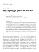
Figure 5: Five noisy LR were synthetically generated by random warp and downsampling by 2, additive Gaussian noise (σ
2
= 40), and 1
outlier image. (a) Reference LR image, SNR
= 11.85. (b) SR result with mean fusing (ML solution) after 10 iterations, SNR = 14.12. (c)
Iterative median fusing after 10 iterations, SNR
= 15.32.(d)SRusingadaptiveFIRfilteringafter10iterations,SNR= 15.99.
to apply space filling curves that are defined over arbitrary
sized images, for example the scanning technique that is pro-
posed in [19] provides an elegant method for preserving two-
dimensional continuity.
To further enhance the stability of the LMS estimator, the
adapted FIR coefficients are saved in between successive iter-
ations of the super-resolution algorithm. These are used to
initialize the input coefficients at the beginning of each scan-
ning block. In fact, in the presence of consistent outliers, the
coefficients tend to stabilize quickly after scanning through
a small part of the image (see Figure 6), and the outlier re-
gions can be pointed out, since their corresponding coeffi-
cients are much smaller than the rest. The detected outlier
regions can be thrown away w hen processing the following it-
erations to reduce the computational complexity of the over-
all algorithm.
6. SIMULATION RESULTS
In this section, we show the performance of the proposed
technique. First, we tested the algorithm on a sequence of
synthetic test images. The images, 5 in total, were generated
from a single HR image according to the imaging model de-

scribedin(1). The original HR image was randomly warped
using an 8 parameter projective model. The registration pa-
rameters were saved for the reconstruction experiments. We
used a continuous Gaussian psf (psf
= 0.5) as the blurring
operator, and we downsampled the images by 2 to obtain
the 5 LR images. All images were contaminated with additive
Gaussian noise (σ
2
= 40). Out of the 5 obtained images, we
singled out one image, and we introduced a deliberate error
in its registration parameter corresponding to a translation
error of 1.5 pixels on the LR image grid.
We ran the algorithm on the resulting set of images.
Figure 6 shows the trajectory of the adapted coefficients
through the first iteration. In this experiment, we fixed a
small LMS step size, γ
= 5 · 10
−7
. Although the step size is
relatively small, the LMS estimator successfully singles out
the outlier image (third image) by decreasing its correspond-
ing FIR coefficient a(3) after scanning through a small part
of the image.
We compared the results of iterative super-resolution
obtained using the proposed fusing process against the mean
and median filters. For the three compared techniques, we
used the same step size μ
n
i

in the update (4). Figure 5 shows
the result images; both our fusing technique and the median
fusing successfully singled out the outlier image and im-
proved the robustness of the overall SR process. Compared
to median fusing, the proposed filtering has shown better
robustness towards noise, and was able to reconstruct finer
character details. Figure 7 shows the corresponding SNR
values across the iterations. The SNR figures confirm that
the proposed filtering scheme consistently performs better
than the mean and median filters. It is worth mentioning
that the intermediate result was truncated in between iter-
ations, which helped to constrain the solution and achieve
steadier convergence for this set of almost binary images.
Note that in all experiments, we have not used a regular-
ization operator because we are mainly interested to isolate
the effect of the fusing strategy. We assume that it would
be possible to enhance the final result when we correctly
assert some prior knowledge about the image content in the
regularization step.
8 EURASIP Journal on Applied Signal Processing
0
0.05
0.1
0.15
0.2
0.25
FIR coefficient values
0 4000 8000 12000 16000
Scan path, in pixels (k)
a(1) a(4)

a(2)
a(3)
a(5)
Coefficient trajectory through first iteration
step size
= 0.5e − 7
Image 3 corresponds to the outlier image
Figure 6: Adaptation of the filter coefficients during the first iter-
ation corresponding to the image shown in Figure 5(d). The coef-
ficient a(3) reflecting the contribution of the outlier image is auto-
matically decreased.
12
12.5
13
13.5
14
14.5
15
15.5
16
SNR
0123456789
Iterations
SNR adaptive FIR fusing gradient images
SNR median fusing of gradient images
SNR average fusing of gradient images
Figure 7: SNR comparison across the first 10 iterations for the
super-resolved images shown in Figure 5. SNR curves for (a) pro-
posed adaptive solution, (b) median fusing of the gradient images,
and (c) average fusing of the gradient images.

In Figure 8, we repeated the same experiment. We gener-
ated 4 LR images with the same parameters described above,
but in this setting, we selected the last LR frame, and we in-
serted several outlier objects. Figure 10 shows the SNR val-
ues across the iterations for the three fusing techniques. The
convergence of the SR algorithm is fast during the first 4
iterations of the steepest descent (SD), but in the follow-
ing iterations, the SNR starts to oscillate without significant
improvement. This example illustrates the need for a reg-
ularization step in order to ensure the convergence of the
solution. Early abortion of the iterations is the only avail-
able option to avoid over-amplified edges. In Figure 8,we
display the results after 4 iterations, again, both the me-
dian and the proposed solution eliminated the outlier ar-
eas, whereas the mean failed. Better SNR performance, as
well as better visual result, was obtained with our fusing
method (Figure 8(f)). Figure 9 shows the trajectory of the
adapted coefficients through the last iteration. The coeffi-
cient a(4) reflecting the contribution of the last LR image is
automatically decreased when stepping inside an outlier area.
When the scanning steps outside the outlier area, the co-
efficient increases again. The other coefficients correspond-
ing to the nonoutlier images are kept around the same level.
As indicated in Figure 9, basically our method oper ates as a
weighted mean filter, except for the detected outlier areas.
So, compared to median fusing, an improved performance
against Gaussian noise is predictable. In Figure 8(f), the ex-
pert eye will notice some artifacts near the borders of the
Hilbert scanning blocks that contain outlier regions. These
are due to the fast and abrupt change of the coefficient values

on the borders of the subareas that were used for scanning. To
reduce this effect, some implementation enhancements can
be designed, such as the use of larger scanning areas or the
smoothing of the coefficients near adjacent blocks.
Figure 11 shows the super-resolved images obtained us-
ing 5 LR scenery images taken with a camera phone (Nokia
6600). To register the pixels on the reference HR grid, we used
hierarchical block matching in the centra l parts of the image,
followed by the estimation of the global projective motion
parameters. In one of the images, the registration failed due
to a significant perspective change. Figure 11(a) shows the
interpolated reference frame (pixel replication). Figure 11(b)
shows the result when simple mean fusing is used; note the
picture of a ghost car that does not belong to the original
scene. Figures 11(c) and 11(d) show, respectively, the results
after 5 iterations when fusing with the median and with the
proposed technique. For both images, the sharpness of the
scene detail is significantly enhanced and the outlier region
in the bottom of the image is successfully eliminated. In this
specific set of input images, the clouds were particularly dif-
ficult to register because they were deformed from one shot
to the next. In fact, for the corresponding area, the only in-
formation that needs to be considered is the one that comes
from the reference frame. This specific example illustrates the
inadequacy of the median filter to fuse this kind of fuzzy re-
gions (Figure 11(c)). Since the input samples do not consti-
tute a reliable majority to obtain a correct vote, the median
filter picks borders randomly from any one of the input im-
ages. The proposed filtering does not solve the problem com-
pletely, however, it prevents the formation of excessive arti-

facts in those reg ions (clouds in Figure 11(d)). The reason is
that similar FIR coefficients are employed when filtering ad-
jacent pixels, unless a clear outlier frame is consistently voted
after scanning through several consecutive pixels, which is
not the case in this example. Note that Zomet et al. [11]have
tackled this problem and proposed to use a bias detection
procedure in conjunction with the median. The detection
procedure outputs a binary mask indicating where to per-
form the filtering. However it is unclear how the thresholds
and the windows would be selected.
Mejdi Trimeche et al. 9
(a) (b) (c)
(d) (e) (f)
Figure 8: (a) Original HR image. (b) The set of LR images used in the experiment: 4 noisy LR were synthetically generated from the original
HR image. The last image was generated from the same image with artificial objects inserted. All images were shifted, downsampled by 2,
and contaminated with additive Gaussian noise (σ
2
= 40). (c) Interpolated reference image (pixel replication), SNR = 8.6. (d) SR result
using iterative mean fusing after 4 iterations, SNR
= 11.4. Remark the shaded outlier regions. (e) SR result using iterative median fusing
after 4 iterations, SNR
= 11.3. (f) SR using adaptive FIR filtering after 4 iterations, SNR = 12.1.
0
0.05
0.1
0.15
0.2
0.25
0.3
0.35

FIR coefficient values
012345678
×10
4
Scan path, in pixels (k)
a(1)
a(2)
a(3)
a(4)
Coefficient trajectory through last iteration
Figure 9: Adaptation of the filter coefficients during the fourth and
last iteration corresponding to the result in Figure 8(f). The coeffi-
cient a(4) reflecting the contribution of the last LR image is auto-
matically decreased when inside an outlier region, when the scan-
ning steps outside the outlier area, the coefficient increases again.
16
× 16 Hilbert scanning is used in this example.
Figure 12 shows a similar example depicting the perfor-
mance of the proposed algorithm on real image scenes. We
used 5 LR images that were cropped from VGA pictures
9
9.5
10
10.5
11
11.5
12
12.5
13
SNR

012345678910
Iterations
SNR for adaptive fusing of gradient images
SNR for median fusing of gradient images
SNR for mean fusing of gradient images
Figure 10: SNR comparison across the first 10 iterations for the
super-resolved images shown in Figure 8. SNR curves for (a) pro-
posed adaptive solution, (b) median fusing of the gradient images,
and (c) average fusing of the gradient images.
imaged at close range (the images are JPEG compressed at
90%). The last frame contained an outlier object. Again, note
that the median fusing (c) and our technique (d) successfully
10 EURASIP Journal on Applied Signal Processing
(a) (b)
(c) (d)
Figure 11: The super-resolved images using the proposed implementation. Five LR images were used. The global motion estimation failed
to register at least one fr ame. (a) Interpolated reference frame, zoom factor 2; (b) result using mean fusing; (c) result using median fusing;
and (d) super-resolved image using the proposed algorithm.
(a) (b)
(c) (d)
Figure 12: The super-resolved images using the proposed implementation. We used 5 LR Images that were cropped from VGA images taken
with a camera phone (Nokia 9500). One outlier object appears in the last frame. (a) Zero-order interpolated reference frame, zoom factor 2;
(b) result using mean fusing, (c) using median fusing, and (d) super-resolved image using the proposed algor ithm.
Mejdi Trimeche et al. 11
wiped out the outlier object from the reconstructed scene.
Looking more closely, we can notice that the result image of
the proposed filtering method has less noise artifacts, espe-
cially on smooth areas.
7. CONCLUSION
In this paper, we have proposed to use adaptive FIR filter-

ing of the gradient images in iterative super-resolution. The
FIR coefficients are adapted using an LMS estimator that is
tuned to detect motion outliers. The algorithm performs ad-
equately in the presence of Gaussian noise, and is capable of
automatically isolating outlier regions, which are due to reg-
istration errors. The proposed method is useful to enhance
the robustness of super-resolution implementations.
ACKNOWLEDGMENT
The authors would like to thank the anonymous reviewers
for their valuable comments and insightful steering to en-
hance the content of this paper.
REFERENCES
[1] R. Y. Tsai and T. S. Huang, “Multiframe image restoration and
registration,” in Advances in Computer Vision and Image Pro-
cessing, vol. 1, chapter 7, pp. 317–339, JAI Press, Greenwich,
Conn, USA, 1984.
[2] S. Chaudhuri, Ed., Super-Resolution Imaging,KluwerAcadem-
ic, Boston, Mass, USA, 2001.
[3] S. C. Park, M. K. Park, and M. G. Kang, “Super-resolution im-
age reconstruction: a technical overview,” IEEE Signal Process-
ing Magazine, vol. 20, no. 3, pp. 21–36, 2003.
[4] S. Baker and T. Kanade, “Super-resolution optical flow,” Tech.
Rep. CMU-RI-TR-99-36, Robotics Institute, Carnegie Mellon
University, Pittsburgh, Pa, USA, 1999.
[5] R. R. Schultz and R. L. Stevenson, “Extraction of high-resolu-
tion frames from video sequences,” IEEE Transactions on Im-
age Processing, vol. 5, no. 6, pp. 996–1011, 1996.
[6] R. C. Hardie, K. J. Barnard, and E. E. Armstrong, “Joint MAP
registration and high-resolution image estimation using a se-
quence of undersampled images,” IEEE Transactions on Image

Processing, vol. 6, no. 12, pp. 1621–1633, 1997.
[7] E. S. Lee and M. G. Kang, “Regularized adaptive high-resolu-
tion image reconstruction considering inaccurate subpixel
registration,” IEEE Transactions on Image Processing, vol. 12,
no. 7, pp. 826–837, 2003.
[8] S. Baker and T. Kanade, “Limits on super-resolution and how
to break them,” IEEE Transactions on Pattern Analysis and Ma-
chine Intelligence, vol. 24, no. 9, pp. 1167–1183, 2002.
[9] S. Farsiu, D. Robinson, M. Elad, and P. Milanfar, “Robust shift
and add approach to super-resolution,” in Applications of Digi-
tal Image Processing XXVI, vol. 5203 of Proceedings of SPIE,pp.
121–130, San Diego, Calif, USA, August 2003.
[10] S. Farsiu, M. D. Robinson, M. Elad, and P. Milanfar, “Fast and
robust multiframe super-resolution,” IEEE Transactions on Im-
age Processing, vol. 13, no. 10, pp. 1327–1344, 2004.
[11] A. Zomet, A. Rav-Acha, and S. Peleg, “Robust super-
resolution,” in Proceedings of IEEE Computer Soc iety Confer-
ence on Computer Vision and Pattern Recognition (CVPR ’01),
vol. 1, pp. 645–650, Kauai, Hawaii, USA, December 2001.
[12] J. Astola and P. Kuosmanen, Fundamentals of Nonlinear Digital
Filtering, CRC Press, New York, NY, USA, 1997.
[13] M. Trimeche and J. Yrj
¨
an
¨
ainen, “Order filters in super-
resolution image reconstruction,” in Image Processing: Algo-
rithms and Systems II, vol. 5014 of Proceedings of SPIE,pp.
190–200, Santa Clara, Calif, USA, January 2003.
[14] D. Capel and A. Zisserman, “Super-resolution from multi-

ple views using learnt image models,” in Proceedings of IEEE
Computer Society Conference on Computer Vision and Pattern
Recognition (CVPR ’01), vol. 2, pp. 627–634, Kauai, Hawaii,
USA, December 2001.
[15] M. Elad and A. Feuer, “Super-resolution reconstruction of im-
age sequences,” IEEE Transactions on Pattern Analysis and Ma-
chine Intelligence, vol. 21, no. 9, pp. 817–834, 1999.
[16] M. Bertero and P. Boccacci, Introduction to Inverse P roblems
in Imaging, chapter 6, Institute of Physics Publishing (IOP),
Bristol, UK, 1998.
[17] S. Haykin, Adaptive Filter Theory, Prentice-Hall, Englewood
Cliffs, NJ, USA, 3rd edition, 1996.
[18] N. Max, “Visualizing Hilbert curves,” in Proceedings of IEEE
Visualization ’98, pp. 447–450, 564, Research Triangle Park,
NC, USA, October 1998.
[19] A. Perez, S. Kamata, and E. Kawaguchi, “Peano scanning of
arbitrary size images,” in Proceedings of 11th IAPR-IEEE Inter-
national Conference on Pattern Recognition (ICPR ’92), vol. 3,
pp. 565–568, The Hague, the Netherlands, August–September
1992.
Mejdi Trimeche received the B.S. degree in
electrical engineering from Bilkent Univer-
sity, Ankara, Turkey, in 1998. In 2000, he
received the M.S. degree with distinction
from the Department of Information Tech-
nology, Tampere University of Technology
(TUT), Tampere, Finland. He is currently
a Ph.D. student with the same university.
He joined Nokia in 2000. Since then, he has
been working in various topics on image

and video processing. Currently, he works as a Senior Research
Engineer in Nokia Research Center. His research interests include
image and video processing, in particular, algorithms for image
restoration and enhancement. Other active topics of interest in-
clude computer vision and content-based indexing and retrieval.
Radu Ciprian Bilcu received the B.S. and
M.S. degrees from the Technical Univer-
sity of Cluj-Napoca, Romania, in 1995 and
1996, respectively, and the Dr.Tech. degree
from Tampere University of Technology,
Tampere, Finland, in 2004. He has pub-
lished 28 papers in international journals
and conferences and holds three patents.
From 1999 to 2004 he was a Researcher at
the Institute of Signal Processing, Tampere
University of Technology, where he was also involved in teaching.
In 2004, he joined Nokia Research Center as a Research Engineer in
the field of image processing. His research interests include adaptive
systems, adaptive algorithms and applications to image processing,
communications, echo control, audio, and speech.
12 EURASIP Journal on Applied Signal Processing
Jukka Yrj
¨
an
¨
ainen studied for the degree
of Engineering Diploma in Tampere Uni-
versity of Technology. He joined Nokia in
1992. Currently he works as a Senior Tech-
nology Manager in Nokia Technology Plat-

forms, Tampere, Finland. He is responsible
for imaging and video related R&D activi-
ties. His interests include image and video
signal processing, multimedia applications,
camera technologies, and processing archi-
tectures for multimedia.