Báo cáo hóa học: "Iterative Refinement Methods for Time-Domain Equalizer Design" potx
Bạn đang xem bản rút gọn của tài liệu. Xem và tải ngay bản đầy đủ của tài liệu tại đây (1.03 MB, 12 trang )
Hindawi Publishing Corporation
EURASIP Journal on Applied Signal Processing
Volume 2006, Article ID 43154, Pages 1–12
DOI 10.1155/ASP/2006/43154
Iterative Refinement Methods for
Time-Domain Equalizer Design
G
¨
uner Arslan,
1
Biao Lu,
2
Lloyd D. Clark,
3, 4
and Brian L. Evans
5
1
Silicon Laboratories, Corporate Headquarters, 7000 West William Cannon Drive, Austin, TX 78735, USA
2
Schlumberger Sugar Land Product Center, 110 Schlumberger Drive, Sugar Land, TX 77478, USA
3
Schlumberger Austin Systems Center, 8311 N FM 620 Road, Austin, TX 78726, USA
4
TICOM Geomatics, 9130 Jollyville Road, Austin, TX 78759, USA
5
Department of Electrical and Computer Engineering, The University of Texas, Austin, TX 78712-1084, USA
Received 1 December 2004; Revised 23 May 2005; Accepted 2 August 2005
Commonly used time domain equalizer (TEQ) design methods have been recently unified as an optimization problem involving an
objective function in the form of a Rayleigh quotient. The direct generalized eigenvalue solution relies on matrix decompositions.
To reduce implementation complexity, we propose an iterative refinement approach in which the TEQ length starts at two taps
and increases by one tap at each iteration. Each iteration involves matrix-vector multiplications and vector additions with 2
× 2
matrices and two-element vectors. At each iteration, the optimization of the objective function either improves or the approach
terminates. The iterative refinement approach provides a range of communication performance versus implementation complexity
tradeoffs for any TEQ method that fits the Rayleigh quotient framework. We apply the proposed approach to three such TEQ
design methods: maximum shortening signal-to-noise ratio, minimum intersymbol interference, and minimum delay spread.
Copyright © 2006 G
¨
uner Arslan et al. This is an open access article distributed under the Creative Commons Attribution License,
which permits unrestricted use, distribution, and reproduction in any medium, provided the original work is properly cited.
1. INTRODUCTION
Multicarrier modulation is a widely used modulation me-
thod for reliable high-speed communication. Discrete multi-
tone (DMT) modulation is a popular variant of multicarrier
modulation that has been standardized for asymmetric and
very high-speed digital subscriber loops (ADSL and VDSL,
resp.) [1]. In these applications, a guard sequence known as
the cyclic prefix is prepended to each symbol to help the re-
ceiver eliminate intersymbol interference (ISI) and perform
symbol recovery.
A DMT symbol consists of N samples, and the cyclic pre-
fix is a copy of the last ν samples of the symbol. The length
of the channel impulse response has to be less than or equal
to (ν + 1) samples in order for all ISI to be eliminated. Using
a cyclic prefix, however, reduces the channel throughput of
a DMT transceiver by a factor of ν/(N + ν). Therefore, it is
desirable to choose ν as small as possible.
The ADSL and VDSL standards set ν to be N/16. In
the field, however, ADSL and VDSL channel impulse re-
sponses can exceed N/16 samples. It is up to the equalizer
in the receiver to shorten the channel impulse response and
to correct for frequency distortion in the shortened channel.
These two equalization tasks may be decoupled or combined
[2]. In a decoupled approach, the equalizer is a cascade of
a time-domain equalizer (TEQ) to shorten the channel, a fast
Fourier transform (FFT) to perform multicarrier demodula-
tion, and a frequency-domain equalizer (FEQ) to invert the
frequency response of the shortened channel [3]. These three
operations are linear. Combined equalization approaches ex-
ploit the linearity by either moving the TEQ into the FEQ
to yield per-tone equalizers [4], or moving the FEQ into the
TEQ to yield complex-valued time-domain equalizer filter
banks [5]. Combined equalization approaches yield higher
data rates than decoupled approaches for the downstream
ADSL case [2].
A TEQ is generally implemented as a finite impulse re-
sponse (FIR) filter placed at the receiver. The cascade of the
channel impulse response and the TEQ forms an effective
channel impulse response with length of ν + 1 samples, as
shown in Figure 1. (In the case of ADSL, the channel im-
pulse response is actually shortened to ν samples.) Various
design criteria resulting in many different design methods
have been proposed to calculate the TEQ coefficients [3, 6–
8]. These four cited desig n methods can be unified as an op-
timization problem involving a Rayleigh quotient [2]. The
generalized eigenvalue solution using matrix decompositions
2 EURASIP Journal on Applied Signal Processing
×10
−3
2
1.5
1
0.5
0
−0.5
−1
−1.5
−2
Amplitude
0 50 100 150 200 250 300
Discrete time
Original channel
Shortened channel
Figure 1: Example of the channel impulse response (carrier serving
area loop 1), and the shortened channel impulse response obtained
with a 16-tap TEQ designed with a maximum shortening signal-to-
noise ratio (MSSNR) method.
is in general not practical to implement in real-time on pro-
grammable digital signal processors.
Instead, iterative design methods could be a pplied. The
iterative method could fix the TEQ length, N
w
,andusegra-
dient descent based on the Rayleigh quotient formulation to
iterate towards an optimal answer [9]. The step size must
be chosen with care, and scaling (normalization) may be
needed at each iteration. Although each iteration depends on
matrix-vector multiplications and vector additions involving
N
w
× N
w
matrices and vectors of length N
w
,matrixdecom-
positions are avoided.
We propose an iterative refinement approach in which
the TEQ length starts at two taps and increases by one tap at
each iteration. A maximum TEQ length may be set. Other
stopping criteria include the cases in which no significant
improvement in the objective function over the previous
iteration, and cases in which the objective function value
has degraded over the previous iteration. Hence, the ap-
proach will improve the design at each iteration until it ter-
minates. No step size needs to be chosen and no scaling
is needed. Each iteration involves matrix-vector multiplica-
tions and vector additions but involving 2
× 2matricesand
two-element vectors. Provided that the proposed approach
completes its initialization step, the proposed approach can
be terminated at any time and a useful TEQ will result.
Hence, our approach scales with the available computational
resources.
We apply the iterative refinement approach to the objec-
tive functions of three different TEQ design methods: max-
imum shortening signal-to-noise ratio (MSSNR) [6], min-
imum intersymbol interference (min-ISI) [7], and mini-
mum delay spread (MDS) [8] methods. For each TEQ de-
sign method, we develop two iterative refinement algorithms.
The divide-and-conquer Rayleigh quotient (DC-Rayleigh)
algorithm uses the objective function in Rayleigh quotient
form. The divide-and-conquer eigenvector algorithm (DC-
eigenvector) optimizes the numerator of the objective func-
tion subject to a constraint involving the TEQ. The DC-
eigenvector algorithm will have lower implementation com-
plexity than the DC-Rayleigh algorithm, which in turn will
have significantly lower complexity than the originally re-
ported TEQ design method.
The rest of the paper is organized as follows. Section 2
summarizes the three TEQ design methods of interest with
their objective functions. Section 3 derives the closed-form
solutions for the DC-Rayleigh and DC-eigenvector meth-
ods. Section 4 applies the DC-Rayleigh and DC-eigenvector
methods to three TEQ design methods. Section 5 shows de-
tailed simulation results for the proposed methods. Section 6
concludes the paper.
2. BACKGROUND
In this section, we summarize three existing TEQ design
methods and the objective functions they optimize. All
methods assume that ν is the length of the cyclic prefix, that
the equalized or effective channel impulse response has a to-
tal delay of Δ samples, and that perfect knowledge of the
channel impulse response is available. In ADSL and VDSL,
the channel impulse response can be estimated during train-
ing. During training, the discrete Fourier transform (DFT)
of the channel impulse response is estimated, from which we
can obtain the channel impulse response estimate. The ef-
fect of channel estimation error on the following TEQ design
methods has been quantified in [10].
2.1. The maximum shortening signal-to-noise
ratio method
Melsa et al. [6] approach the TEQ design as solely a chan-
nel shortening problem. They define a shortening signal-to-
noise (SSNR) and derive the optimal TEQ in terms of maxi-
mizing SSNR which is the ratio of the energy inside a win-
dow of (ν + 1) samples starting at sample (Δ + 1) to the
energy outside the same window of the shortened channel
impulse response. An ideal shortened channel impulse re-
sponse would be zero-valued outside the window in order to
yield zero ISI and infinite SSNR. The assumption is that the
larger the SSNR, the closer the shortened channel impulse re-
sponse is to the ideal. However, optimizing SSNR is not nec-
essarily equivalent to maximizing bitrate or minimizing bit-
error rate but only an approximation to make the TEQ design
problem mathematically tra ctable. Although this method ig-
nores all noise components simulation results show that it
performs comparably well to other methods that take noise
into account [2].
Let us define the effective or shortened channel impulse
response h
eff
(k)as
h
eff
(k) = h(k) ∗ w(k), (1)
G
¨
uner Arslan et al. 3
where h(k) is the channel impulse response of length L
h
,
w(k) represents the N
w
TEQ coefficients, and “∗”denotes
linear convolution. We can represent h
eff
(k)invectorform
as
h
eff
=
h
eff
(1), h
eff
(2), , h
eff
L
h
+ N
w
− 1
. (2)
The goal is to choose the TEQ coefficients such that the en-
ergy of the effective channel impulse response h
eff
mostly
concentrates inside a window with length ν + 1, one sample
longer than the cyclic prefix. To accomplish this goal, we split
h
eff
into two parts, h
win
and h
wall
, which represent samples of
the effective channel impulse response inside and outside the
window [6], respectively:
h
win
=
h
eff
(Δ+1), h
eff
(Δ +2), , h
eff
(Δ + ν +1)
,
h
wall
=
h
eff
(1), , h
eff
(Δ), h
eff
(Δ+ν +2), , h
eff
L
h
+ N
w
− 1
.
(3)
The samples in h
wall
include the samples before the window
and the samples after the window. The SSNR objec tive func-
tion [6]isdefinedas
SSNR
= 10 log
10
Energy in h
win
Energy in h
wall
,(4)
where h
win
and h
wall
can be written in matrix form as shown
in the following:
⎡
⎢
⎢
⎢
⎢
⎣
h
eff
(Δ +1)
h
eff
(Δ +2)
.
.
.
h
eff
(Δ + ν +1)
⎤
⎥
⎥
⎥
⎥
⎦
h
win
=
⎡
⎢
⎢
⎢
⎢
⎣
h(Δ +1) h(Δ) ··· h
Δ − N
w
+2
h(Δ +2) h(Δ +1) ··· h
Δ − N
w
+3
.
.
.
.
.
.
.
.
.
.
.
.
h(Δ + ν +1) h(Δ + ν)
··· h
Δ + ν − N
w
+2
⎤
⎥
⎥
⎥
⎥
⎦
H
win
⎡
⎢
⎢
⎢
⎢
⎣
w(0)
w(1)
.
.
.
w
N
w
− 1
⎤
⎥
⎥
⎥
⎥
⎦
w
(5)
⎡
⎢
⎢
⎢
⎢
⎢
⎢
⎢
⎢
⎢
⎢
⎣
h
eff
(1)
.
.
.
h
eff
(Δ)
h
eff
(Δ + ν +2)
.
.
.
h
eff
L
h
+ N
w
− 1
⎤
⎥
⎥
⎥
⎥
⎥
⎥
⎥
⎥
⎥
⎥
⎦
h
wall
=
⎡
⎢
⎢
⎢
⎢
⎢
⎢
⎢
⎢
⎢
⎢
⎣
h(1) 0 ··· 0
.
.
.
.
.
.
.
.
.
.
.
.
h(Δ) h(Δ
− 1) ··· h
Δ − N
w
+1
h(Δ + ν +2) h(Δ + ν +1) ··· h
Δ + ν − N
w
+3
.
.
.
.
.
.
.
.
.
.
.
.
00
··· h
L
h
− 1
⎤
⎥
⎥
⎥
⎥
⎥
⎥
⎥
⎥
⎥
⎥
⎦
H
wall
⎡
⎢
⎢
⎢
⎢
⎣
w(0)
w(1)
.
.
.
w
N
w
− 1
⎤
⎥
⎥
⎥
⎥
⎦
w
. (6)
The energy of h
win
and h
wall
in (4)canbewrittenas
h
T
wall
h
wall
= w
T
H
T
wall
H
wall
w = w
T
Aw,
h
T
win
h
win
= w
T
H
T
win
H
win
w = w
T
Bw,
(7)
where the N
w
× N
w
matrices are defined as
A
= H
T
wall
H
wall
B = H
T
win
H
win
.
(8)
Note that both A and B are real, symmetric and positive def-
inite (excluding the case of ideal equalization which is not
possible in practice) by definition. SSNR can then be written
in compact form as
SSNR
= 10 log
10
w
T
Bw
w
T
Aw
. (9)
This form is known as the Rayleigh quotient. The optimal
shortening method would find w to minimize w
T
Aw while
satisfying w
T
Bw = 1[6]. Solving this problem via the La-
grange multiplier method easily yields the solution that w
should be chosen as the generalized eigenvector of B and A
corresponding to the largest generalized eigenvalue [11].
The approach in [6] to find the solutions is based on the
assumption that B is positive definite so that it has a Cholesky
decomposition as, B =
√
B
√
B
T
.Then,l
min
is computed as
the eigenvector associated with the smallest eigenvalue of the
matrix (
√
B)
−1
A(
√
B
T
)
−1
. Finally, w
opt
= (
√
B
T
)
−1
l
min
.
Amorecomplicatedmethodin[6]applieswhenB is sin-
gular. In order to avoid B from being singular, Yin and Yue
[12] suggest an objective function to maximize w
T
Bw while
satisfying the constraint w
T
Aw = 1. In this case, they as-
sume that A is positive definite since they perform a Cholesky
decomposition on A.Bothcases[6, 12] require a Cholesky
decomposition, an eigendecomposition, and a matrix inver-
sion of an N
w
× N
w
matrix to find w
opt
.
2.2. The minimum intersymbol interference method
Arslan et al. [7] propose a TEQ design method that can
be viewed as a generalization to the MSSNR method. The
minimum intersymbol interference (min-ISI) method is also
4 EURASIP Journal on Applied Signal Processing
a simplified version of the maximum bitrate TEQ [7]design
method that directly optimizes bitrate based on a subchannel
SNR model:
SNR
i
=
S
x,i
C
signal,i
2
S
n,i
C
noise,i
2
+ S
x,i
C
ISI,i
2
, (10)
where S
x,i
, S
n,i
, C
signal,i
, C
noise,i
,andC
ISI,i
are the signal power,
noise power, signal path gain, noise path gain, and ISI path
gain in the ith subchannel, respectively. The min-ISI method
makes use of the observation that the ISI term in the sub-
channel SNR model is the dominant factor limiting bitrate;
hence, minimizing ISI alone would be a viable alternative to
the Maximum Bit Rate (MBR) method [7] that otherwise re-
quires nonlinear optimization to calculate the TEQ taps. The
objective function for the min-ISI method can also be writ-
ten as a Rayleigh quotient with matrices A and B defined as:
A
= H
T
D
T
i∈R
f
H
i
S
x,i
f
i
DH,
B
= H
T
win
H
win
,
(11)
where H is the channel convolution matrix, H
win
is defined
in (5), f
i
is the ith row of the N ×N DFT matrix, and D is a
diagonal matrix where the diagonal is defined a s
g
k
=
⎧
⎨
⎩
0, Δ +1≤ k ≤ Δ + ν +1,
1, otherwise.
(12)
Compared to the MSSNR method, the min-ISI method holds
the energy inside the window of size (ν + 1) constant while
minimizing a frequency-weighted form of the energy outside
the window. The frequency weighting is based on the signal
energy at a given frequency bin which can be thought as the
ISI energy. The weighting can also be chosen to take channel
noise into account by replacing S
x,i
in (11)withS
x,i
/S
n,i
where
S
n,i
is the noise power in subchannel i. This weighting func-
tion emphasizes the placement of ISI in the frequencies with
high SNR (low noise power). A small amount of ISI power
in subchannels with low noise power can reduce the overall
SNR dramatically. In subchannels with low SNR, however,
the noise power is large enough to dominate the ISI power
such that the effect of ISI power on the SNR is negligible.
2.3. The minimum delay spread method
Schur and Speidel [8] propose another approach to shorten
a channel impulse response which can be described as vari-
ation of the MSSNR method. The idea behind this approach
is to minimize the square of the delay spread of the effective
channel impulse response w hich is defined as
D
=
1
E
L
c
n=0
(n − n)
2
c[n]
2
, (13)
where c is the effective channel impulse response defined as
c
= Hw. L
c
is the length of the effective channel impulse
response, E
= c
T
c is the total energy in the effective channel
impulse response, and
n is the predefined “center of mass.”
If we can think of the MSSNR method as weighting the
samples of the effective channel impulse response with zero
inside the window of size ν + 1 and one elsewhere, the MDS
method, on the other hand, weights all samples with the
square distance from the “center of mass” which has a similar
function to the Δ delay parameter in the MSSNR or min-ISI
methods. The objective function of this method is the square
delay spread which can be written as a Rayleigh quotient with
A and B defined as
A
= H
T
QH,
B
= H
T
H,
(14)
where Q is a diagonal matrix with the diagonal made of the
vector [(0
− n)
2
,(1− n)
2
, ,(L
w
+ L
h
−1 − n)
2
], and n is the
“center of mass.”
3. DIVIDE-AND-CONQUER METHODS
Each method in the previous section requires a Rayleigh
quotient to be optimized. The solution to this optimiza-
tion problem is a generalized eigenvector of the two m atri-
ces. Computing the generalized eigenvectors is a computa-
tionally challenging task that requires a heavy computational
burden and careful scaling to prevent singularities in the
matrix computations. In this section, we propose two sub-
optimal methods called the divide-and-conquer Rayleigh-
quotient (DC-Rayleigh) and divide-and-conquer eigenvec-
tor (DC-eigenvector) methods that can be used with most
objective functions that can be written as a Rayleigh quotient.
The proposed DC methods divide the calculation of a N
w
-
tap TEQ into smaller problems of finding two-tap TEQs, one
per iteration. A unit-tap constraint is placed on each two-tap
TEQ. The proposed methods are computationally efficient
and do not require any advanced matrix computation that
could cause singularity problems.
3.1. Divide-and-conquer Rayleigh quotient method
The goal is to optimize an objective function of the form
J
=
w
T
Aw
w
T
Bw
. (15)
At the ith iteration, w
i
is a 2 ×1 vector (a two-tap equalizer),
and A
i
and B
i
are 2 × 2 matrices. Assuming a unit-tap con-
straint on each w
i
:
w
i
=
1, g
i
T
(16)
the objective function becomes
J
i
=
w
T
i
A
i
w
i
w
T
i
B
i
w
i
=
1 g
i
a
1,i
a
2,i
a
2,i
a
3,i
1
g
i
1 g
i
b
1,i
b
2,i
b
2,i
b
3,i
1
g
i
=
a
1,i
+2a
2,i
g
i
+ a
3,i
g
2
i
b
1,i
+2b
2,i
g
i
+ b
3,i
g
2
i
.
(17)
G
¨
uner Arslan et al. 5
Table 1: DC-Rayleigh algorithm steps and complexity analysis for MSSNR, min-ISI, and MDS TEQ design, only step 3.1 differs among the
TEQ methods.
Step Description Multiplications Additions Divisions Square root
1 Initialize w
TEQ
= [1]— ———
2 Initialize h
0
= h ————
3 Repeat for i
= 1, , N
w
− 1— — — —
3.1 MSSNR A
i
(28)andB
i
(29)2(L
h
+ i +1) 2(L
h
+ i)— —
3.1 min-ISI A
i
(30)andB
i
(29)2(L
h
+ i + N +2) 2(L
h
+ i + N +1) — —
3.1 MDS A
i
(32)andB
i
(33)5(L
h
+ i)+4 5(L
h
+ i)— —
3.2 g
i,1
and g
i,2
from (19)14 8 21
3.3 J in (25)forg
i,1
and g
i,2
12 8 2 —
3.4 w
TEQ
= w
TEQ
∗ w
i
(i −1) (i −1) — —
3.5 h
i
= h
i−1
∗ w
i−1
(L
h
+ i)(L
h
+ i)——
The assumption that matrix B is positive definite prevents the
denominator in (17) from going to zero for any value of g
i
.
Inspection of the B matrices in the three objective functions
in the previous section will show that all are symmetric and
positive definite by definition.
Differentiating J
i
in (17)withrespecttog
i
, setting the
derivative to zero, and simplifying the result leads to
a
3,i
b
2,i
− a
2,i
b
3,i
g
2
i
+
a
3,i
b
1,i
− a
1,i
b
3,i
g
i
+
a
2,i
b
1,i
− a
1,i
b
2,i
=
0.
(18)
The solutions to the quadratic function of g
i
in (18)are
g
i,(1,2)
=
−
a
3,i
b
1,i
− a
1,i
b
3,i
±
γ
2
a
3,i
b
2,i
− a
2,i
b
3,i
, (19)
where γ is
a
3,i
b
1,i
− a
1,i
b
3,i
2
− 4
a
3,i
b
2,i
− a
2,i
b
3,i
a
2,i
b
1,i
− a
1,i
b
2,i
.
(20)
We choose the value of g
i
among {g
i,1
, g
i,2
} in (19) that gives
the optimal value for J
i
. Once the value for g
i
is chosen,
we have a two-tap TEQ w
i
that maximizes the given objec-
tive.
Our goal is to maximize the objective for a N
w
-tap TEQ.
After the first iteration, we convolve the calculated two-tap
TEQ with the channel impulse response h to obtain an in-
termediate effective channel impulse response h
1
. Assuming
that this newly calculated intermediate effective channel im-
pulse response is our new channel we repeat the above proce-
dure and calculate a new two-tap TEQ and a new intermedi-
ate channel impulse response. This process is repeated N
w
−1
times so that we have g
i
, and hence w
i
for i = 1, , N
w
− 1.
The N
w
-tap TEQ can than be obtained by convolving all two-
tap TEQs together:
w(k)
= w
1
(k) ∗ w
2
(k) ∗···∗w
N
w
−1
(k), (21)
where w
i
(k) is the two-tap TEQ obtained at the ith iteration.
Table 1 summarizes the steps of the DC-Rayleigh method.
We can also design a t wo-tap equalizer with a unit-norm
constraint (UNC) as
w
i
=
sin θ
i
,cosθ
i
T
. (22)
By factoring out sin θ
i
,wecanrewrite(22)toobtain
w
i
=
sin θ
i
,cosθ
i
T
= sin θ
i
1,
cos θ
i
sin θ
i
T
= sin θ
i
1, η
i
T
.
(23)
If we substitute (23) into (17), then the sin θ
i
term would can-
cel out, which would give the same result as (19).
3.2. Divide-and-conquer eigenvector method
The DC-Rayleigh method finds a suboptimal solution of an
objective funct ion described as a Rayleigh quotient. In many
cases, however, the denominator term of the objective func-
tion is constrained to prevent the trivial all-zero TEQ solu-
tion. For example in the MSSNR and min-ISI methods the
denominator term is to constrain the energy inside the win-
dow of length ν + 1. In the MDS method the denominator is
constraining the total energy in the effective channel impulse
response. The D C-Rayleigh method already places a unit-tap
constraint on each two-tap TEQ, which prevents the trivial
solution.
The DC-eigenvector method is developed to drop the de-
nominator term from the objective function and optimize
the numerator only in order to prevent over-constraining
the solution space. The problem is reduced to optimizing the
quadratic objective function
J
i
= w
T
i
A
i
w
i
. (24)
We apply the same idea in optimizing this objective func-
tion by defining a two-tap TEQ as in (16) and rewriting the
6 EURASIP Journal on Applied Signal Processing
objective function at the ith iteration as
J
i
= w
T
i
A
i
w
i
=
1 g
i
a
1,i
a
2,i
a
2,i
a
3,i
1
g
i
=
a
1,i
+2a
2,i
g
i
+ a
3,i
g
2
i
.
(25)
Differentiating J
i
in (25)withrespecttog
i
and setting the
derivative to zero gives
g
i
=−
a
2,i
a
3,i
. (26)
Once again we obtain the optimal solution for a two-tap
TEQ. Repeating this process N
w
− 1 times and convolving
the resulting two-tap TEQs together, we obtain the N
w
-tap
TEQ.
Note that the DC-Rayleigh method requires the calcula-
tion of all entries of both A and B matrices at e very iteration,
but the DC-eigenvector method only requires two entries of
the A matrix to be computed in every iteration. The DC-
eigenvector method also does not require a square root oper-
ation, which further reduces the computational complexity
and is more suitable for real-time implementation on a pro-
grammable digital signal processor.
Similar to the DC-Rayleigh method we can derive the
unit-norm constrained DC-eigenvector by replacing w
i
in
(25)by(23)toobtain
J
i,UNC
= w
T
i
A
i
w
i
= sin θ
i
1 η
i
a
1,i
a
2,i
a
2,i
a
3,i
sin θ
i
1
η
i
=
sin
2
θ
i
a
1,i
+2a
2,i
η
i
+ a
3,i
η
2
i
(27)
which will make η
i
equal to g
i
in (26)afterwesolvefor
η
i
. Therefore, both unit-tap constraint and unit-norm con-
straint in DC-Rayleigh and DC-eigenvector methods should
yield the same per formance.
4. APPLICATION OF DIVIDE-AND-CONQUER
METHODS
This section gives detailed derivations on how the MSSNR,
min-ISI, and MDS objective functions can be used in con-
junction with DC-Rayleigh and DC-eigenvector methods.
Tables 1 and 2 describe the steps and quantify the
computations per iteration for the DC-Rayleigh and DC-
eigenvector methods, respectively. Note that only the calcu-
lation of the A
i
and B
i
matrices differ between methods.
The delay parameter (Δ in the min-ISI and MSSNR
methods or
n in the MDS method) is still an important pa-
rameter in the DC methods although it does not appear in
the derivation of the DC methods themselves. This param-
eter is embedded in the A
i
and B
i
matrices, as it was in the
original methods. In [2], a range of 15–35 for the delay pa-
rameter caused a change in achieved bitrate of less than
±1%
for MDS,
±2% for MSSNR, and ±5% for min-ISI methods.
A reasonable initial guess for the delay parameter is the cyclic
prefix length ν (i.e., 32 for downstream ADSL). When using
the DC methods, a delay search could be performed during
the first iteration.
4.1. Application to MSSNR
In the case of MSSNR, the A
i
and B
i
matrices used at iteration
i are written as
A
i
= H
T
i,win
H
i,win
=
a
1,i
a
2,i
a
2,i
a
3,i
=
⎡
⎢
⎢
⎢
⎢
⎢
⎢
⎣
Δ+ν+1
k=Δ+1
h
2
i
(k)
Δ+ν+1
k=Δ+1
h
i
(k)h
i
(k − 1)
Δ+ν+1
k=Δ+1
h
i
(k)h
i
(k − 1)
Δ+ν+1
k=Δ+1
h
2
i
(k − 1)
⎤
⎥
⎥
⎥
⎥
⎥
⎥
⎦
,
(28)
B
i
= H
T
i,wall
H
i,wall
=
b
1,i
b
2,i
b
2,i
b
3,i
=
⎡
⎢
⎢
⎢
⎣
k∈S
h
2
i
(k)
k∈S
h
i
(k)h
i
(k − 1)
k∈S
h
i
(k)h
i
(k − 1)
k∈S
h
2
i
(k − 1)
⎤
⎥
⎥
⎥
⎦
,
(29)
where h
i
(k) = h
i−1
(k) ∗ w
i
(k)fori = 1, , N
w−1
, k =
0, , L
h
+ i − 1, and h
0
(k) is the original channel impulse
response. The convolution to obtain the new intermediate
channel impulse response is simplified by the fact the first
tap of the two-tap TEQ is always set to one; hence, only one
multiplication and one addition is required to calculate each
tap of the new intermediate impulse response. Also note that
a
3,i
and b
3,i
are closely related to a
1,i
and b
1,i
,respectively,in
that they differ in only two elements of the sums hence can
be derived from each other without recomputing the square
of the sums.
4.2. Application to min-ISI
In the case of min-ISI, the B
i
matrix is the same as given in
(29) and the elements of A
i
are defined as
a
1,i
=
k∈R
N−1
n=0
h
i
(n)s(k − n)
2
,
a
2,i
=
k∈R
N−1
n=0
h
i
(n)s(k − n)
N−1
n=0
h
i
(n)s(k − 1 − n)
2
,
a
3,i
=
k∈R
N−1
n=0
h
i
(n)s(k − 1 − n)
2
,
(30)
where S
={1, , Δ, Δ + ν +2, , N} and s(n) is the time-
domain equivalent of the frequency-domain weighting func-
tion S
x,i
andisdefinedas
s(n)
=
N−1
i=0
S
x,i
e
j(2π/N)in
. (31)
The application of DC methods to the min-ISI objective
function requires first the calculation of the time-domain
weighting function s(n), which can be performed with an
N-point inverse FFT. This calculation needs to b e done only
G
¨
uner Arslan et al. 7
Table 2: Implementation complexity of DC-eigenvector algorithms for MSSNR, min-ISI, and MDS TEQ design methods. Only step 3.1
differs among the TEQ methods.
Step Description Multiplications Additions Divisions Square root
1 Initialize w
TEQ
= [1]— — ——
2 Initialize h
0
= h ————
3FixΔ.Fori
= 1, , N
w
− 1— — ——
3.1 MSSNR A
i
(28)(L
h
+ i − ν)(L
h
+ i − ν −1) — —
3.1 min-ISI A
i
(30)(L
h
+ i − ν)+2(N +1) (L
h
+ i − ν −1) + 2(N +1) — —
3.1 MDS A
i
(32)3(L
h
+ i)+2 3(L
h
+ i)——
3.2 g (26)— —1—
3.3 w
TEQ
= w
TEQ
∗ w
i
(i −1) (i − 1) — —
3.4 h
i
= h
i−1
∗ w
i−1
(L
h
+ i)(L
h
+ i)——
once and not for every iteration. However the inner sums
in (30) are required for every iteration which adds to the
computational complexity compared to the MSSNR objec-
tive function. As a side benefit, the DC methods get around a
restriction of the min-ISI method that the TEQ length could
exceed the CP length by designing two taps at a time.
4.3. Application to MDS
For the MDS objective functions, the A
i
and B
i
matrix ele-
ments are defined as
a
1,i
=
L
c
k=0
(k − n)
2
h
2
i
(k),
a
2,i
=
L
c
k=0
(k − n)(k − 1 − n)h
i
(k)h
i
(k − 1),
a
3,i
=
L
c
k=0
(k − 1)(k − 1 − n)
2
h
2
i
,
(32)
b
1,i
=
L
c
k=0
h
2
i
(k),
b
2,i
=
L
c
k=0
h
i
(k)h
i
(k − 1),
b
3,i
=
L
c
k=0
h
2
i
(k − 1).
(33)
As with the MSSNR method the calculation of both a
3,i
and
b
3,i
can be based on a
1,i
and b
1,i
, respectively, to avoid recal-
culating the sum of squares. Even with these savings, how-
ever, the MDS method requires all sums to be over the entire
length of the intermediate channel impulse response dou-
bling the computational complexity compared to the former
two methods.
4.4. Comparison of computational complexity
We compare the computation complexity of the applica-
tion of both the DC-Rayleigh and DC-eigenvector meth-
ods to all three objective functions in this section. For a fair
comparison of computational complexity, we replace the
eigenvalue decomposition in the original methods by the it-
erative power method [13] since only the dominant eigen-
value and its corresponding eigenvector are needed. We as-
sume 10 iterations for the power method as in [14].
Table 3 summarizes the original TEQ design methods
and their computational costs, whereas Tables 1 and 2 sum-
marize the DC-Rayleigh and DC-eigenvector methods and
their computational complexity, respectively.
Both proposed methods have reduced computational
complexity when compared to the original methods and are
better suited for real-time implementation on digital signal
processors because they avoid any matrix calculations that
require careful scaling. The complexity gap between the orig-
inal and proposed methods increases with increasing N
w
be-
cause the dominant cost savings are from the matrix opera-
tions performed on N
w
× N
w
matrices in the original meth-
ods.
Table 4 lists the computational complexity for each of the
methods for a moderate length TEQ of size N
w
= 16 and
N
= L
h
= 512, and ν = 32, by assuming 10 iterations in the
power method for the orig inal methods. T he largest com-
plexity reduction is 24% and 15% for the MSSNR objective
function for the DC-Rayleigh and DC-eigenvector methods,
respectively. Percentage savings in all cases would increase for
longer TEQs.
5. SIMULATION RESULTS
We showed in the previous section that the divide-and-
conquer methods, especially the DC-eigenvector method,
have significant complexity savings over the original meth-
ods. In this section, we present simulation results to analyze
the bitrate performance of the proposed methods. It is worth
noting that the DC-Rayleigh method communication per-
formance is bounded above by the perfor mance of the origi-
nal method used because it optimizes the same function but
two taps at a time. Since we fix the previous taps at every
iteration, we are not guaranteed to obtain the optimal solu-
tion. It is not possible to determine the upper-bound perfor-
mance for the DC-eigenvector method in terms of the origi-
nal methods since the DC-eigenvector method uses different
constraints compared to the original methods.
8 EURASIP Journal on Applied Signal Processing
Table 3: Implementation complexity of the MSSNR, min-ISI, and MDS methods.
Step Description Multiplications Additions Divisions
1 A and B for MSSNR (8) N
w
(L
h
+2N
w
− 2) N
w
(L
h
+2N
w
− 3) —
1
A and B for min-ISI (11) N
w
(L
h
+2N
w
− 1+N) N
w
(L
h
+2N
w
− 2+N)—
1
A and B for MDS (14)2N
w
(L
h
+2N
w
− 2) + L
h
+ N
w
− 12N
w
(L
h
+2N
w
− 3) + L
h
+ N
w
− 1—
2 Cholesky Decomposition B N
3
w
N
3
w
—
3 (
√
B)
−1
[11](5N
3
w
+ N
w
)/3(5N
3
w
+ N
w
)/3—
4 c = (
√
B)
−1
A(
√
B
T
)
−1
2N
3
w
2N
2
w
(N
w
− 1) —
6 Power method to find eigenvector corresponding to the minimum eigenvalue of C
6.1 Calculate C
−1
[11](5N
3
w
+ N
w
)/3(5N
3
w
+ N
w
)/30
6.2
Initialize l
(0)
———
6.3
z
(k)
= C
−1
l
(k−1)
N
2
w
(N
w
− 1)N
w
0
6.4
l
(k)
opt
= z
(k)
/ z
(k)
N
w
N
w
− 1 N
w
6.5 λ
(k)
= [l
(k)
]
T
C
−1
l
(k)
(N
w
+1)N
w
N
2
w
− 10
6.6
if |λ
(k)
− λ
(k−1)
| > threshold, go to step 6.3 — — —
7 w
opt
= (
√
B
T
)
−1
l
(k)
opt
N
2
w
(N
w
− 1)N
w
0
Table 4: Tradeoff between bitrate performance and complexity
(multiplications) of the original and the two divide-and-conquer
variations of each TEQ design method for ν
= 32, N
w
= 16, and
L
h
= 512. Complexity of original methods assume that the power
method is run for 10 iterations.
Method
Bitrate
(Mbps)
Complexity Bitrate Complexity
MSSNR original 7.96 101 808 100% 100%
MSSNR Rayleigh 7.34 23 925 92% 24%
MSSNR eigenvector 7.74 15225 97% 15%
Min-ISI original 8.02 110 016 100% 100%
Min-ISI Rayleigh 7.40 39 315 92% 36%
Min-ISI eigenvector 7.70 30615 96% 28%
MDS original 7.72 111 007 100% 100%
MDS Rayleigh 7.45 47 355 96% 43%
MDS eigenvector 7.58 31 335 98% 28%
All simulations are based on the commonly used eight
carrier-serving-area (CSA) loops that were obtained from
the UT Austin Matlab DMTTEQ Toolbox [15]. The CSA
loops are placed in cascade w ith two fifth-order high-pass
Chebyshev filters. The first filter has a turn-on frequency of
4.8 kHz and simulates the effect of the splitter that separates
the voice-band from the data-band. The second filter is used
to separate the upstream from the downstream in frequency
division multiplexing at a frequency of 138 kHz.
A transmit signal power of 26 dBm on a 100 Ω load is
assumed. The thermal noise is modeled as white Gaussian
noise with
−140 dBm/Hz spectral power. Near-end crosstalk
noise is introduced for 8 ISDN disturbers as described in the
ADSL specifications [1].Allmethodsmakeuseofanideal
estimate of the channel impulse response.
The delay parameter is chosen based on a heuristic search
that gives satisfactory performance with minimal complexity
[14]. The method uses a rectangular window of size ν +1
that is slid over the original channel impulse response so that
the SSNR as defined in (4) is maximized. The index of the
first nonzero sample of the w indow is chosen as the delay
parameter.
Simulations are carried out for 300 DMT symbols carry-
ing quadrature phase-shift key ing (QPSK) signals in all sub-
channels, except for subchannel 0 (voiceband) which is not
used for data, subchannels 1–5 (ISDN band) which are not
used for data, and subchannel N/2 + 1 which cannot carry
complex symbols. At the receiver, an FIR TEQ filters the re-
ceived noisy signal, and passes its output through the cyclic
prefix removal block and the FFT. A one-tap FEQ per sub-
channel rotates the symbols in each subchannel. (We de-
signed the FEQ tap on each subchannel to be optimal in
a mean-squared error sense.) The rotated symbols are then
compared to the transmitted symbols in each subchannel,
and the difference is the error signal, from which the receiver
SNR is calculated. Based on the SNR in each subchannel, we
calculate the total bitrate achievable for the given TEQ by us-
ing
b
DMT
=
k∈R
log
2
1+
SNR
i
Γ
, (34)
where R is a set of indices for all used subchannels, SNR
i
is
the SNR in subchannel i, and the SNR gap Γ is 10.8dB[16].
Figure 1 shows the impulse response of CSA loop 1
and the shortened or effective impulse response obtained
with a 16-tap TEQ designed with the proposed MSSNR-
DC-Rayleigh method. Figure 2 compares the performance
of all nine methods for all 8 CSA loops with the matched-
filter bound (MFB) and the case where no TEQ is used at
all. The motivation of using a TEQ is apparent due to the
gap in communication performance when no TEQ is used.
When comparing the original methods among each other in
achieved bitrate, the MSSNR and min-ISI methods perform
closely while outperforming the MDS method. All meth-
ods seem to perform relatively close to the MFB although
other TEQ design methods that get even closer to the MFB
G
¨
uner Arslan et al. 9
10
9
8
7
6
5
4
3
2
1
0
Bitrate (Mbps)
12345678
CSA loop
MFB
MSSNR
MINISI
MDS
MSSNR-RQ
MINISI-RQ
MDS-RQ
MSSNR-EV
MINISI-EV
MDS-EV
NO-TEQ
Figure 2: Performance of all methods on 8 CSA loops with TEQ
length N
w
= 16, symbol length N = 512, channel length L
h
= 512,
and cyclic prefix length ν
= 32.
exist [2]. As expected, the proposed suboptimal div ide-and-
conquer methods generally perform worse than the orig-
inal methods. However, on CSA loops 6 and 8, the pro-
posed MDS-DC-eigenvector method actually outperforms
the original MDS method. This could be expected since none
of the methods directly optimize bitrates but alternative ob-
jective functions such as the delay spread in this case. Since
optimizing the delay spread is not equivalent to optimizing
the bitrate, one can sometimes expect the bit rate to increase
while the delay spread decreases.
Another observation from Figure 2 is that most of the
time, the DC-eigenvector method outperforms the DC-
Rayleigh method. At first thought, one might think that
the DC-Rayleigh method should perform better because it
solves the original objective functions as opposed to a sim-
plified one, as the DC-eigenvector method does. As men-
tioned in Section 3.2, the DC-Rayleigh method may be over-
constraining the solution due to the new constraint on the
first tap of the two-tap equalizers designed at every iteration.
For all three original methods in this paper, the denominator
of the Rayleigh quotient serves mostly as a constraint to pre-
vent the all-zero trivial solution for the TEQ. The divide-and-
conquer methods already have a unit-tap constraint built
into them. Thus, removing the original constraint expands
the solution space, and the DC-eigenvector method is able to
find better solutions most of the time while having lower im-
plementation complexity. Taking into account the reduction
in computational complexity when compared to the DC-
Rayleigh method the DC-eigenvector method seems to be a
better choice in general.
The primary motivation of the proposed DC methods
is to reduce the computational complexity and avoid ma-
trix computations that require careful scaling in return for
some communication performance loss. Figure 3(a) maps all
methods referred in this paper onto a two-dimensional space
with one axis representing the computational complexity and
the other communication performance. The best solutions
would lie in the lower right corner of this map where perfor-
mance is maxima and computational complexity is minimal.
This plot is obtained by averaging the bitrate numbers ob-
tained for each method on each of the eight CSA loops. We
see from this plot that the MSSNR-DC-eigenvector method is
the choice when computational complexity is the major de-
ciding factor. If, however, communication performance is the
only factor, then the original min-ISI or the MSSNR meth-
ods seemed to be the best choice. Complexity of the original
methods assume that the power method is run for 10 itera-
tions. One could easily argue that the performance gap be-
tween the proposed DC methods and the original methods
is so small (on the order of 0.5 Mbps) that the extra com-
plexity and implementation hardship due to matrix opera-
tions is not justified. This plot also reveals that for all DC-
Rayleigh methods there exists a method that gets better per-
formance with lower computational complexity. A similar ar-
gument holds for the min-ISI objective function which seems
not to perform as well as the other two objective functions
when DC methods are applied. The MSSNR-DC-eigenvector
method gives on average better performance with less com-
plexity compared to the min-ISI when DC methods are ap-
plied. Figure 3(b) shows performance for all methods un-
der varying numbers of TEQ taps. The graph shows that
most methods settle around an upper-bound performance
with a 10-tap TEQ. The DC-Rayleigh methods actually re-
duce bitrate performance with increasing numbers of taps.
This again could be explained by the fact that none of these
methods directly optimize the bitrate. It turns out that the
DC-Rayleigh method tends to use the additional freedom of
more TEQ taps in the wrong direction in terms of bitrate
performance.
Finally we analyze the effect of channel estimation error
on each method. The channel estimation error is modeled
as additive white Gaussian noise on the ideal (real) channel
impulse response. The noisy channel estimate is used in the
calculations of the TEQ coefficients with each method while
the performance estimation is done using the real channel
impulse response.
As shown in Figure 4 the performance of all methods in-
creases with increasing SNR of the channel estimation error.
For SNRs higher than 80 dB the original methods outper-
form the iterative methods by similar margin as with an ideal
channel so the noise is too low to have an effect on the results.
The performance gap between the original and DC meth-
ods increases for SNRs lower than 80 dB–90 dB. The worst-
case additional performance loss of the DC methods over the
original methods is around 3% for the MSSNR and min-
ISI-based DC methods and about 14% for the MDS-based
DC methods. So we can conclude that the MDS method is
more sensitive to channel estimation errors w hen used in
conjunction with the proposed DC methods. This conclu-
sion also agrees with the results in [10].
Although the DC-Rayleigh method fol lows the trend of
the original method with drastic performance reductions at
lower SNRs, the DC-eigenvector method delivers about 30–
40% of the peak bitrate even with bad channel estimates. This
again may be explained by the fact that the DC-eigenvector
10 EURASIP Journal on Applied Signal Processing
×10
4
12
10
8
6
4
2
0
Complexity (number of multiplications)
7.47.67.888.2
Bitrate (Mbps)
MSSNR
MINISI
MDS
MSSNR-RQ
MINISI-RQ
MDS-RQ
MSSNR-EV
MINISI-EV
MDS-EV
(a)
8
7.5
7
6.5
6
5.5
Achievable bit rate (Mbps)
51015202530
Number of TEQ taps (N
w
)
MSSNR
MSSNR-EV
MSSNR-RQ
(b)
8
7.5
7
6.5
6
5.5
Achievable bitrate (Mbps)
51015202530
Number of TEQ taps (N
w
)
MINISI
MINISI-EV
MINISI-RQ
(c)
8
7.5
7
6.5
6
5.5
Achievable bitrate (Mbps)
51015202530
Number of TEQ taps (N
w
)
MDS
MDS-EV
MDS-RQ
(d)
Figure 3: With symbol length N = 512 and channel length L
h
= 512, communication performance versus (a) implementation complexity
for all methods with TEQ length N
w
= 16 and cyclic prefix length ν = 32, where the bitrates are taken as the average over all eight CSA
loops; (b) TEQ length for MSSNR methods; (c) TEQ length for min-ISI methods; and (d) TEQ length for MDS methods. EV means the
DC-eigenvalue method and RQ means the DC-Rayleigh method.
methods are less constrained hence have a larger space to find
a better solution even with noisy channel estimates. The orig-
inal methods as well as the DC-Rayleigh methods practically
stop working at low SNR situations delivering only about
10% of the peak bitrate with 20 dB estimation noise.
6. CONCLUSION
The design of a time-domain equalizer (TEQ) for dis-
crete multitone modulation has been studied extensively and
a number of methods can deliver bitrates close to the up-
per bound of achievable performance. Many of these high-
performance methods can mathematically be classified as an
optimization of a Rayleigh quotient, which requires com-
putationally intensive matrix decompositions to solve di-
rectly. The focus of this paper is to reduce the computational
complexity by avoiding matrix decompositions. We propose
an iterative refinement approach in which the TEQ length
starts at two taps and increases by one tap at each itera-
tion.
G
¨
uner Arslan et al. 11
10
5
0
Achievable bitrate (Mbps)
20 30 40 50 60 70 80 90 100
Channel estimation SNR (dB)
MSSNR
MSSNR-EV
MSSNR-RQ
(a)
10
5
0
Achievable bitrate (Mbps)
20 30 40 50 60 70 80 90 100
Channel estimation SNR (dB)
MINISI
MINISI-EV
MINISI-RQ
(b)
10
5
0
Achievable bitrate (Mbps)
20 30 40 50 60 70 80 90 100
Channel estimation SNR (dB)
MDS
MDS-EV
MDS-RQ
(c)
Figure 4: Performance of all methods on CSA loop 1 with TEQ length N
w
= 16, symbol length N = 512, channel length L
h
= 512, cyclic
prefix length ν
= 32, and SNR of channel estimation error. Estimation error is modeled as additive white Gaussian noise. Performance is
averaged over 10 runs.
The first method is the divide-and-conquer Rayleigh
quotient (DC-Rayleigh) method. The DC-Rayleigh gives an
approximate solution to the Rayleigh quotient optimization
problem. Our simulation results show that the proposed DC-
Rayleigh method gives close to ideal performance with re-
duced computational complexity. The fact that the proposed
DC-Rayleigh method introduces an additional unit-tap con-
straint on the solutions motivates us to fur ther simplify the
TEQ design methods by dropping the divisor term from the
Rayleigh quotient. This yields to a quadratic cost functions
with eigenvector solutions. The second method is the divide-
and-conquer eigenvector method (DC-eigenvector), which
solves the eigenvalue problem approximately with further re-
duced complexity.
We apply both divide-and-conquer methods to optimize
the objective functions of three different TEQ design meth-
ods. The methods are the maximum shortening signal-to-
noise ratio, minimum intersymbol interference, and mini-
mum delay spread (MDS). Complexity analysis and simu-
lations results show that the proposed methods reduce the
computational complexity of the original methods with mi-
nor performance degradation. In fact, the proposed itera-
tive refinement approach provides a range of communication
performance versus implementation complexity tradeoffsfor
any TEQ method that fits the Rayleigh quotient framework.
The measure of communication performance depends on
the objective function used by the TEQ method.
REFERENCES
[1] “ANSI T1.413-1995, Network and customer installation in-
terfaces: Asymmetrical digital subscr iber line (ADSL) metal-
lic interface,” printed from: Digital Subscriber Line Technol-
ogybyT.Starr,J.M.Cioffi, and P. J. Silverman, Prentice-Hall,
1999.
[2] R. K. Martin, K. Vanbleu, M. Ding, et al., “Unification and
evaluation of equalization structures and design algorithms
for discrete multitone modulation systems,” IEEE Transac-
tions Signal Processing, vol. 53, no. 10, part 1, pp. 3880–3894,
2005.
[3] J. S. Chow and J. M. Cioffi,“Acost-effective maximum likeli-
hood receiver for multicarrier systems,” in Proceedings of IEEE
International Conference on Communications (ICC ’92), vol. 2,
pp. 948–952, Chicago, Ill, USA, June 1992.
[4] K. Van Acker, G. Leus, M. Moonen, O. van de Wiel, and T.
Pollet, “Per tone equalization for DMT-based systems,” IEEE
Transactions on Communications, vol. 49, no. 1, pp. 109–119,
2001.
[5] M. Ding, Z. Shen, and B. L. Evans, “An achievable per-
formance upper bound for discrete multitone equalization,”
in Proceedings of IEEE Global Telecommunications Conference
(GLOBECOM ’04), vol. 4, pp. 2297–2301, Dallas, Tex, USA,
November–December 2004.
[6]P.J.W.Melsa,R.C.Younce,andC.E.Rohrs,“Impulsere-
sponse shortening for discrete multitone transceivers,” IEEE
Transactions on Communications, vol. 44, no. 12, pp. 1662–
1672, 1996.
12 EURASIP Journal on Applied Signal Processing
[7] G. Arslan, B. L. Evans, and S. Kiaei, “Equalization for discrete
multitone transceivers to maximize bit rate,” IEEE Transactions
Signal Processing, vol. 49, no. 12, pp. 3123–3135, 2001.
[8] R. Schur and J. Speidel, “An efficient e qualization method to
minimize delay spread in OFDM/DMT systems,” in Proceed-
ings of IEEE International Conference on Communications (ICC
’01), vol. 5, pp. 1481–1485, Helsinki, Finland, June 2001.
[9] R. K. Martin, K. Vanbleu, M. Ding, et al., “Implementation
complexity and communication performance tradeoffs in dis-
crete multitone modulation equalizers,” to appear in IEEE
Transactions Signal Processing, />bevans/papers/2005/equalizationII.
[10] M. Ding, B. L. Evans, and I. Wong, “Effect of channel estima-
tion error on bit rate performance of time domain equalizers,”
in Proceedings of 38th IEEE Asilomar Conference on Signals,
Systems and Computers, vol. 2, pp. 2056–2060, Pacific Grove,
Calif, USA, November 2004.
[11] G. H. Golub and C. F. Van Loan, Matrix Computation,John
Hopkins University Press, Baltimore, Md, USA, 3rd edition,
1996.
[12] C. Yin and G. Yue, “Optimal impulse response shortening for
discrete multitone transceivers,” IEE Electronics Letters, vol. 34,
no. 1, pp. 35–36, 1998.
[13] J. W. Demmel, Applied Numerical Linear Algebra,SIAM,
Philadelphia, Pa, USA, 1997.
[14]B.Lu,L.D.Clark,G.Arslan,andB.L.Evans,“FastTime-
Domain Equalization for Discrete Multitone Modulation Sys-
tems,” in Proceedings of IEEE Digital Signal Processing Work-
shop, Hunt, Tex, USA, October 2000.
[15] G. Arslan, M. Ding, B. Lu, M. Milosevic, Z. Shen, and B.
L. Evans, “MATLAB DMTTEQ Toolbox 3.1,” 2003, Available
at: />∼bevans/projects/adsl/dmtteq/
dmtteq.html.
[16] N. Al-Dhahir and J. M. Cioffi, “A bandwidth-optimized
reduced-complexity equalized multicarrier transceiver,” IEEE
Transactions on Communications, vol. 45, no. 8, pp. 948–956,
1997.
G
¨
uner Arslan received his Ph.D. degree in
electrical engineering (2000) at the Uni-
versity of Texas at Austin in Austin, Texas,
USA. His dissertation was entitled Equal-
ization for Discrete Multitone Transceivers.
He received his M.S. degree in electron-
ics and communications engineering from
Yildiz Technical University, Istanbul, Turkey
in 1998, and his B.S. degree in electronics
and communications engineering as Vale-
dictorian of his class from Yildiz University, Kocaeli, Turkey in
1994. He is currently a Senior Systems Design Engineer in the wire-
less product division of Silicon Laboratories based in Austin, Texas,
USA. He is also an Adjunct Faculty in the Electrical and Computer
Engineering Depart ment at the University of Texas at Austin. His
research interests are in digital signal processing, communications
systems, and embedded real-time digital signal processing. He is
a Member of IEEE Signal Processing and Communication Soci-
eties.
Biao Lu received her Ph.D. degree in elec-
trical engineering (2000) and M.S.E.E. de-
gree (1997) from the University of Texas at
Austin in Austin, Texas, USA. Her disserta-
tion was entitled Wireline Channel Estima-
tion and Equalization. She received her B.S.
degree in biomedical engineering (1992)
from the Capital Institute of Medicine in
Beijing, China. Since 2000, she has been
with Schlumberger in Houston, Texas, USA,
where she is currently a Senior Software Engineer in telemetry sys-
tems. Her research interests include signal processing, image pro-
cessing, neural networks, and embedded systems.
Lloyd D. Clark received his B.S., M.S., and
Ph.D. degrees in electrical engineering and
computer science from the Massachusetts
Institute of Technology in 1984, 1986, and
1990, respectively. From 1990 to 2003, he
held various positions at the Schlumberger
Austin Technology Center in Austin, Texas,
USA, including Principal Engineer and Re-
search Scientist. While at Schlumberger, he
designed and developed wireline telemetry
systems for well logging applications for the oil field, as well as
wireless metering systems. Since 2004, he has been a Principal Sci-
entist with Ticom Geomatics in Austin, Texas, USA, where he has
been the technical lead on several wireless geolocation projects. He
holds several patents, has published several technical papers, and
has coadvised graduate students at both MIT and t he University of
Texas at Austin.
Brian L. Evans is Professor of Electrical
and Computer E ngineering at the Univer-
sity of Texas at Austin in Austin, Texas,
USA. His B.S.E.E.C.S. ( 1987) degree is from
the Rose-Hulman Institute of Technology in
Terre Haute, Indiana, USA, and his M.S.E.E.
(1988) and Ph.D.E.E. (1993) degrees are
from the Georgia Institute of Technology in
Atlanta, Georgia, USA. From 1993 to 1996,
he was a Postdoctoral Researcher at the Uni-
versity of California, Berkeley, in design automation for embedded
digital systems. At UT Austin, his research group develops signal
quality bounds, optimal algorithms, low-complexity algorithms,
and real-time embedded software of high-quality image halftoning
for desktop printers, smart image acquisition for digital still cam-
eras, high-bitrate equalizers for multicarrier ADSL receivers, and
resource allocation for multiuser OFDM base stations. He is the
architect of the Signals and Systems Pack for Mathematica. He re-
ceived a 1997 US National Science Foundation CAREER Award.