Báo cáo hóa học: "Efficient Realization of Sigma-Delta (Σ-Δ) Kalman Lowpass Filter in Hardware Using FPGA" ppt
Bạn đang xem bản rút gọn của tài liệu. Xem và tải ngay bản đầy đủ của tài liệu tại đây (1.42 MB, 11 trang )
Hindawi Publishing Corporation
EURASIP Journal on Applied Signal Processing
Volume 2006, Article ID 52736, Pages 1–11
DOI 10.1155/ASP/2006/52736
Efficient Realization of Sigma-Delta (Σ-Δ) Kalman
Lowpass Filter in Hardware Using FPGA
Saman S. Abeysekera and Charayaphan Charoensak
School of Elect rical & Electronic Engineering, Nanyang Technological University, Block S1, Nanyang Avenue, Singapore 639798
Received 8 December 2004; Revised 3 August 2005; Accepted 12 September 2005
Recommended for Publication by Peter Handel
Sigma-delta (Σ-Δ) modulation techniques h ave moved into mainstream applications in signal processing and have found many
practical uses in areas such as high-resolution A/D, D/A conversions, voice communication, and software radio. Σ-Δ modulators
produce a single, or few bits output resulting in hardware saving and thus making them suitable for implementation in very
large scale integration (VLSI) circuits. To reduce quantization noise produced, higher-order modulators such as multiloop and
multistage architectures are commonly used. The quantization noise behavior of higher-order Σ-Δ modulators is well understood.
Based on these quantization noise characteristics, various demodulator architectures, such as sinc filter, optimal FIR filter, and
Laguerre filter are reported in literature. In this paper, theory and design of an efficient Kalman recursive demodulator filter is
shown. Hardware implementation of Kalman lowpass filter, using field programmable gate array (FPGA), is explained. The FPGA
synthesis results from Kalman filter design are compared with previous designs for sinc filter, optimum FIR filter, and Laguerre
filter.
Copyright © 2006 Hindawi Publishing Corporation. All rights reserved.
1. INTRODUCTION
Recently, Σ-Δ modulation techniques have been successfully
applied in numerous applications such as low-cost and high-
resolution A/D and D/A converters, software-defined radio
[1, 2], correlators, multipliers, and synchronizers [3].
One main reason for popularity of Σ-Δ modulation lies
in its ability to trade bandwidth with quantization noise. Σ-
Δ circuit allows reduction in hardware complexity, while at
the same time provides higher signal resolution. The fewer
number of bits removes the need for expensive multibit cir-
cuitry such as multipliers and hence decreases the overall
circuit complexity. In some cases, multipliers can be en-
tirely eliminated from the circuit [4]. These features make
Σ-Δ based circuits attractive for complete system-on-chip
designs [3, 5, 6]. The applications of Σ-Δ require proper low-
pass filters as demodulators to remove quantization noise.
Various demodulator filter architectures, such as optimum
FIR filter, sinc filter, and Laguerre filters are well understood
and reported in literature [7–10].
In this paper, theory and efficient realization of a Kalman
lowpass filter is described and implemented in hardware us-
ing field programmable gate array (FPGA). The simulation
and synthesis results of FPGA implementation of the filter
are reported. Comparison of synthesis results among various
FPGA filter desig ns including sinc filter, optimum FIR filter,
Laguerre filter, and Kalman filters, both down-sampled and
full-rate, is given.
This paper is organized as follows. Section 2 briefs on
some lowpass filters commonly used for removing quantiza-
tion noise from Σ-Δ modulators. Sections 3 and 4 explain,
respectively, Kalman filter and theory formulation of effi-
cient, full-rate implementation of the Kalman filter. Section 5
shows MATLAB simulation of down-sampled and full-rate
Kalman filters. Section 6 describes the FPGA implementation
of full-rate Kalman filter with results of FPGA simulations
and comparison of FPGA resource requirement compared to
previously reported filter designs [11, 12].
2. SOME COMMON LOWPASS FILTER ARCHITECTURES
FOR Σ-Δ DEMODULATION
The single feedback loop Σ-Δ modulator produces a high
quantization noise. The improved signal-to-quantization
noise performance can be achieved by using the multiloop
(DSM) [13] or the multistage (MASH) architectures [14, 15].
The typical quantization noise charac teristics of various Σ-Δ
modulators are described in literature [7].
2 EURASIP Journal on Applied Signal Processing
Let x(n) be a slowly varying input signal to a Σ-Δ modu-
lator. For simplicity, consider the case where x(n)isadcsig-
nal given by x(n)
= ρ. (This assumption is usually warranted
due to the oversampling of Σ-Δ modulator.) The power spec-
trum of the output, y(n), of a Σ-Δ modulator is given by
[11]
S
yy
( f ) =
(2 sin πf)
2m
3
+ ρ
2
δ( f ), (1)
where f denotes the frequency, normalized by the sampling
frequency, and m is the order of the modulator. The second
term of the right-hand side of (1) is the signal term while the
first term represents the quantization noise resulting from
the modulator. The objective is to design a digital filter, H(z),
such that the filtered quantization noise power at the output
of the demodulator is minimized, that is,
Γ
= min
0.5
−0.5
H
e
j2πf
2
(2 sin πf)
2m
df (2)
subject to
H
e
j2πf
|
f =0
= 1. (3)
The linear constraint on the minimization problem of (3)
is imposed to pass dc signal unattenuated through the filter.
The effective bandwidth of the filter is given by
f
B
=
0.5
−0.5
H
e
j2πf
2
df
H
e
j2πf
2
f
=0
. (4)
At the demodulator, the high-frequency noise produced by
the Σ-Δ modulator is removed by using the lowpass filter,
H(z), and the input signal is recovered.
Some common Σ-Δ lowpass filters are introduced in
the following subsections. They are discussed in more de-
tail in literature [9, 10, 16, 17]. The architecture of recursive
Kalman filter is explained in detail in Sections 3 and 4.
2.1. Sinc
K
/ comb filter
An N-tap sinc filter is described by the impulse response:
h(k)
=
1
N
(0
≤ k ≤ N −1). (5)
An N-tap sinc
K
filter is a cascade of K(N/K)-tap filters. The
amplitude response of sinc
K
filter is given by
H( f )
=
K
sin(πfN/K)
N · sin(πf)
K
. (6)
Usually, a sinc
L+1
filter is used to filter out the quantization
noise of an Lth-order modulator.
2.2. Optimum FIR filter
An optimal filter that produces the minimum filtered quanti-
zation noise power at the output can be derived [15, 16]. For
second-order multiloop (DSM2) and third-order multistage
(MASH3) architectures, coefficients of the N-tap optimum
FIR filter are given by
DSM2 : c(n)
=
30
N
n +1
N +1
n +2
N +2
N − n
N +3
×
N +1− n
N +4
,
MASH3 : c(n)
=
140
N
n
N
3
1 −
n
N
3
;0≤ n<N.
(7)
The number of filter taps, N, is usually selected to be the same
as the oversampling ratio (OSR) of the Σ-Δ modulator.
2.3. Optimal Laguerre IIR filter
To minimize quantization noise, it is described in [17, 18]
that the filter transfer function, H(z), can be expressed using
the following truncated Laguerre series:
H
L
(z) =
M−1
k=0
γ
k
φ
k
(z), (8)
where γ
k
is the Laguerre series coefficients and φ
k
(z) is the
frequency domain Laguerre function, given by
φ
k
(z) =
z
√
1 − a
2
z −a
1 − az
z −a
k
,
− 1 ≤ a<1, k = 0, 1, , M −1.
(9)
Using (8), the minimization of noise yields
Γ
= min
˜
γ
T
Q
m
˜
γ
subject to u
T
˜
γ
= h, (10)
where
˜
γ
= [γ
0
, γ
1
, , γ
M−1
]
T
, h =
(1 − a)/(1 + a), u is a
unit vector of length M,andQ
m
is a constant positive definite
matrix.
The quantization noise power resulting from Laguerre
lowpass filter is the same as that resulting from an optimum
FIR filter.
S. S. Abeysekera and C. Charoensak 3
x(n)+
−
+
−
y(n)
Δ
μ(·)
Δ
p(n)
(a)
x
k
y
k
q
k
p
k
Z
−1
1 − Z
−1
+
+
1
− Z
−1
ν
k
+
(b)
Figure 1: (a) Single-loop Σ-Δ modulator and (b) its linear repre-
sentation.
3. KALMAN FILTER
This section will describe the design methodology for the
Kalman lowpass filter that produces minimum filtered quan-
tization noise power at the output. It is first assumed that in
(1) m
= 1, that is, a first-order Σ-Δ modulator is considered.
The design will then be extended to higher-order modula-
tors.
Figure 1(a) shows the first-order (single-loop) Σ-Δ mod-
ulator, where x(n)andp(n) are the input and output sig-
nals, respectively. The input to the threshold element μ(
·)is
denoted y(n). The Σ-Δ modulator in Figure 1(a) is not lin-
ear due to presence of the thresholder. However, the circuit
can be approximated to be linear as shown in Figure 1(b)
[11, 19].
The circuit in Figure 1(b) can be described by two state
variables,
{x
k
, y
k
} corresponding to signals x(n)andy(n)in
Figure 1(a).Hereν
k
denotes the quantization error of the
thresholder, which can be approximately represented as a
white Gaussian process with variance 1/12 [20]. The follow-
ing state-space relationship can be obtained for the circuit in
Figure 1(b):
x
k+1
= x
k
,
y
k+1
= x
k+1
+ y
k
,
q
k
= y
k
+ ν
k
,
(11)
where
q
k
=
1
1 − z
−1
p
k
. (12)
Based on (11), let φ and H be defined as
φ
=
10
11
, H =
[0 1]
T
. (13)
Then, the Kalman gain equation (state update) and the
Kalman prediction equation can be obtained as follows [21]:
K
k
=
φβ
k
φ
T
H
H
T
φβ
k
φ
T
H + σ
2
,
G
k+1
= φG
k
+ K
k
q
k
− H
T
φG
k
,
(14)
0
−20
−40
−60
−80
−100
−120
−140
−160
−180
−200
00.511.52 2.533.54
Iteration number (log)
m.s.e (dB)
Simulation
From theoretical equation
Figure 2: Output mean-squared error (m.s.e) versus iteration num-
ber, m
= 2. Theoretical result is shown for an optimum FIR filter
[19].
where G
k
is the state vector, given by G
k
={x
k
, y
k
}
T
and σ
2
is
the quantization noise variance. Furthermore, the covariance
of the state estimation error β
k
(i.e., the 2×2 state covariance
matrix) satisfies
β
k+1
= γ
I −K
k
H
T
φβ
k
φ
T
(15)
with I being the identity matrix and γ being a forgetting fac-
tor, selected as γ
= 1. Note that p
k
is the output of the mod-
ulator in Figure 1(b),andq
k
is obtained by integrating p
k
.
Taking the quantization noise variance σ
2
= 1/12, and using
the initial conditions shown in (16), it is possible to update
(14)-(15) recursively:
β
k=0
=
1
12
[I]
2×2
, G
k=0
=
[0 0]
T
. (16)
After updating (14)-(15)forN times (where N
= OSR), the
filtered output can be taken from the value of the first el-
ement of the state vector G
k
, that is, G
k
(1), and again the
filter is initialized using the conditions in (16). This pro-
cedure essentially implements lowpass filtering and down-
sampling operations. Extension of Kalman lowpass filter for
the second-order modulator is str aightforward. This could
be obtained by modifying (13)and(16), respectively, as
φ
=
⎡
⎢
⎣
100
110
111
⎤
⎥
⎦
, H =
[0 0 1]
T
,
β
k=0
=
1
12
[I]
3×3
, G
k=0
=
[0 0 0]
T
.
(17)
Extension to higher-order demodulators could be easily ob-
tained via generalization of (17).
For each update (or iteration) the filer output is taken
from the value of G
k
(1). Figure 2 shows the filtered error as
4 EURASIP Journal on Applied Signal Processing
a function of the number of iterations, k of a second-order
modulator (m
= 2) when the forgetting factor is selected as
γ
= 1. Note that the filtered error is the same as that obtained
using the N-length optimal FIR filter defined in ( 7).
Note here that the recursion in (14)-(15)iscompleteat
every N samples (down-sampling), and the m.s.e of Kalman
filter will be the same as that of an optimum FIR filter.
4. FULL-RATE KALMAN FILTER
The previous section discusses the implementation of the
down-sampled Kalman filter. However in certain applica-
tions, a full-rate demodulator filter would be very advan-
tageous. This means that the Σ-Δ demodulator is used at a
sampling frequency given by the OSR. For example, in [5], a
full-rate Laguerre filter has shown to improve the noise per-
formance by approximately 13 dB. In another example [6], a
bandpass Σ-Δ demodulator is used to retrieve the intermedi-
ate frequency (IF) in a software radio system. In this case, full
sampling rate processing would be necessary as frequency es-
timation from the IF signal depends on the number of sam-
ples used. A full-rate lowpass filter would improve the accu-
racy by a factor of N
3
[10]. (For N = 128, SNR will increase
by 63 dB!)
In full-rate applications, the Kalman filter can be imple-
mented such that the recursive formulas in (14)-(15)areup-
dated continuously, without down-sampling, that is, N
→∞.
In such a case where N
→∞, the filter bandwidth and the
mean-squared error of the filtered output approaches zero
(see Figure 2). However, this is not acceptable as it is neces-
sary for the demodulator to have a finite bandwidth so that
the desired signal can pass through the filter.
In the case of optimum FIR filter design, the filter length
is selected as the oversampling ratio (OSR) of the system.
The objective function, Γ, (mean-squared error of the filtered
output) and the bandwidth of the optimum FIR was shown
in Section 2. It is possible to design a Kalman filter with a
finite bandwidth by using appropriate selection of the for-
getting factor γ.
For a second-order modulator, m
= 2, it can be shown
that using the following values for γ, the Kalman filter would
result in the same m.s.e as that of an optimum FIR filter [12]:
γ
=
5.210
N
. (18)
Equation (18) provides the value of the forgetting factor that
needs to be used in the full-rate Kalman filter for a given
oversampling ratio. Figure 3 shows the filtered error as a
function of the number of iterations, for second-order mod-
ulator, w hen the forgetting factor is selected as given in (18).
Efficient full-rate Kalman filter implementation
According to Figure 1(b), the input to the Kalman filter q
k
is obtained as an integrated value of the Σ-Δ modulator out-
put p
k
. The hardware implementation of Kalman filter could
0
−20
−40
−60
−80
−100
−120
−140
−160
−180
−200
00.511.52 2.533.54
Iteration number (log)
m.s.e (dB)
From equation
N
= 32
N
= 128
N
= 512
N
= 2048
Figure 3: Mean-squared error versus iteration number for m = 2.
Forgetting factors are selected using (18).
be improved, however, by moving the demodulator block
(1
− z
−1
) in Figure 1(b) from the demodulator input to the
demodulator output. This avoids the integration of the in-
put signal in the demodulator that would cause significant
bit-growth in the data path in hardware implementations
and thus increases hardware cost. Noting that q
k
= p
k
, the
Kalman filter equations for Figure 1(b) could now be written
as
G
k+1
= φG
k
+ K
k
p
k
− H
T
φG
k
. (19)
Assuming that the steady states have been a chie ved, the out-
put, o
k
, is obtained from integrating the state vector G
k
as
shown in the following:
o
k
= G
k
(1)+G
k−1
(1). (20)
(For a second-order modulator m
= 2, the output is ob-
tained by double integrating the state vector.) This modified
demodulator, thus, avoids integrating the input signal. The
hardware resource can be further reduced by implementing
the demodulator using a preevaluated steady-state Kalman
gain K
∞
(this is elaborated in Section 6.2). The recursive
computations of (14)-( 15) are thus avoided, reducing the
required number of multiplications and results in hardware
saving.
5. PERFORMANCE RESULTS
The proposed recursive Σ-Δ demodulator filter architectures
were implemented and used to filter and down-sample Σ-
Δ-modulated signals from a double-loop modulator (DSM
where m
= 2), where OSR and N = 128. The parameters for
Laguerre filter were selected as a
= 0.906 25, M = 7. The re-
sults from the recursive filters were compared with that from
a 128-tap optimum FIR filter. First, the modulator input was
selected as a dc signal with value 0.0921. The mean-squared
errors of the resulting lowpass filtered down-sampled signals
S. S. Abeysekera and C. Charoensak 5
0
−20
−40
−60
−80
−100
−120
−140
−160
−180
0 5 10 15 20 25
Frequency (kHz)
Power (dB)
Input
From Optimum FIR,
Laguerre
and Kalman filter
Figure 4: Input signal and down-sampled demodulated power
spectra from optimum FIR filter, Laguerre filter, and Kalman filter.
are shown below:
optimum FIR filter
−88 dB,
Laguerre filter
−87 dB,
Kalman filter
−87 dB.
It can be seen that Laguerre filter, Kalman filter, and opti-
mum FIR filter result in similar values of mean-squared er-
rors. (Note that the quantization noise power resulting from
(6)is
−85 dB for a sinc filter.)
Next, in the second simulation, the modulator input was
selected as the sum of three sinusoids, (amplitudes and fre-
quencies of the sinusoids are 0.36, 0.24, 0.18 and 1.44, 6.24,
16.80 kHz, resp.), and sampled at 48 kHz. Figure 4 shows the
demodulated signal power spectra resulting from optimum
FIR filter, Laguerre filter, and Kalman filter.
For comparison, input signal power spectrum is also
shown in Figure 4. The power spectra are computed using
the 1024-point FFT and with Hann window. (Total signal
length is 2048 samples.) Note that optimum FIR filter, La-
guerre filter, and Kalman all produce a noise floor at approx-
imately
−120 dB. Since the FFT length is 1024, the signal-to-
quantization noise ratios resulting from all three filters are
around
−90 dB, which is as expected from previously noted
dc signal simulation. As can be seen from Figure 4, all three
filters produce no signal attenuation.
It has been proposed in [18] to use a Laguerre filter as a
narrowband lowpass postprocessing filter before the down-
sampling operation. In using the Laguerre filter for filtering
the quantization noise, by suitable selection of the Laguerre
filter pole parameter a, the two Laguerre filters (i.e., the op-
timal quantization noise filter and the post-narrowband fil-
ter) could b e combined. This results in efficient hardware ar-
chitecture while improving the signal-to-quantization noise
ratio. The simulation result of this simplified Laguerre archi-
tecture is described next.
The two inputs to the Σ-Δ modulator were the same dc
and complex sinusoid signals used in previous simulations.
0
−20
−40
−60
−80
−100
−120
−140
−160
0 5 10 15 20 25
Frequency (kHz)
Power (dB)
Input
Laguerre without
post-filter
Laguerre with
post-filter
Figure 5: Demodulated signal and input signal power spectra from
Laguerre filters, with and without postprocessing filter.
The modulated signals were lowpass filtered using the opti-
mal Laguerre filter described in Section 2.3. The lowpass fil-
tered signal was down-sampled, with and without the post-
processing narrowband Laguerre filter. The narrowband La-
guerre filter has 21 coefficients [5]. For the dc signal, the m.s.e
results from the two architectures are as follows:
using a single Laguerre filter
−87 dB,
with additional postprocessing filter
−100 dB.
For the three sinusoids input, Figure 5 shows the demod-
ulated signal power spectra from Laguerre filters, with and
without postprocessing narrowband filter. It can be seen that,
by adding the postprocessing Laguerre filter, another 13 dB
of quantization noise reduction is achieved. Note that the
two Laguerre filters could be combined into a single fil-
ter with 27 coefficients [18]. The coefficients of the com-
binedLaguerrefilterare10
−3
[0.0888, 0.3395, 0.5345, 0.2248,
−0.9247, −2.7369, −4.1848, 3.6235, 0.4083, 8.4116, 19.4670,
31.1266, 40.0539, 43.3961]. Due to symmetry of the filter,
only one half of the coefficients are shown.
Figure 6 shows the results from Kalman demodulator.
Asinusoidoffrequency0.13
× 48 = 6.24 kHz, with ampli-
tude 0.5 was used. Figure 6(a) shows the input and demod-
ulated down-sampled output signal spectra, using 64-point
FFT and with Hann window. Figure 6(b) shows the output
spectrum from the full-rate Kalman filter. The figure shows
that by using the full-rate demodulator, approximately an
SNR gain of 15 dB could be obtained.
6. FPGA IMPLEMENTATION OF KALMAN
LOWPASS FILTER
To get insight into hardware implementation of Kalman fil-
ter architecture, this section presents the FPGA design for the
second-order full-rate Kalman lowpass filter described ear-
lier. Although application specific integrated circuit (ASIC)
offers the most efficient hardware implementation, the rapid
realization achieved by using field programmable gate array
6 EURASIP Journal on Applied Signal Processing
−20
−40
−60
−80
−100
−120
00.05 0.10.15 0.20.25 0.30.35 0.40.45 0.5
Frequency (normalized by sampling frequency)
Power (dB)
Input
Down-sampled
Kalman
Error signal
(a)
−20
−40
−60
−80
−100
−120
00.20.40.60.81 1.21.41.61.82
Frequency (normalized by sampling frequency)
Power (dB)
Input signal
Kalman filtered signal
Error signal
(b)
Figure 6: Demodulated signal, input signal, and error power spec-
tra from Kalman filters: (a) down-sampled, (b) full-rate.
(FPGA) is more suitable for prototyping phase in which the
new concept or architecture is verified. Section 6.1 presents
FPGA design and simulation results of the second-order
full-rate Kalman filter. Section 6.2 describes hardware sim-
plifications of the filter. Detailed comparison of FPGA im-
plementations among various architectures is given in Sec-
tion 6.4.
6.1. FPGA implementation of Kalman demodulator
In this experimentation, the FPGA design and simulation
tools used were System Generator version 2.3 from Xilinx
[22], Simulink, and MATLAB version 6.5 from MathWorks.
The second-order down-sampled Kalman filter and full-
rate Kalman filter described in Section 4 were designed using
System Generator. Figure 7 shows the top level of FPGA im-
plementation under Simulink environment of MATLAB. Fig-
ure 8 shows more details of the circuit that implement (19).
The FPGA design of the down-sampled Kalman filter was
then used to filter the Σ-Δ-modulated complex sinusoid sig-
nal described in Section 5. The MATLAB simulation results
from Section 5 and the FPGA simulation results are then
compared.
MATLAB uses double precision floating point numeric
system whereas only fixed-point number is commonly used
in FPGA implementation. In order to compare FPGA result
with MATLAB result, without too much effect of quanti-
zation noise introduced by the fixed-point arithmetic used,
the bit size of data path in FPGA is allowed to grow with-
out truncation, up to 32 bits. No attempts to save the FPGA
gate count were carried out at this point. The optimized
FPGA implementation of the Kalman filter is explained in
Section 6.2.
The input signal to the Σ-Δ modulator was a sum of three
sinusoids, sampled at 48 kHz. Amplitudes and frequencies of
the sinusoids are 0.36, 0.24, 0.18 and 1.44, 6.24, 16.80 kHz,
respectively. The Σ-Δ modulator used was the double-loop
modulator (DSM where m
= 2, referred to as DSM2) with
OSR
= 128. Figure 9 shows the spectrum of the down-
sampled demodulated output signal. The window size of FFT
was 1024, and with Hann window. The SNR achieved is ap-
proximately 100 dB. The FPGA result agrees with the MAT-
LAB simulation shown in Figure 4 in Section 5.
Next, the FPGA design of the second-order full-rate
Kalman filter was simulated and the result compared with
that from the down-sampled Kalman filter. A sinusoid with
frequency 0.13
× 48 = 6.24 kHz, amplitude 0.5, and 48 kHz
sampling frequency was used. Figure 10(b) compares the
error spectrum of the filtered output signal from full-rate
Kalman filter against the input signal of the Σ-Δ modula-
tor. When compared to the same simulation for the down-
sampled Kalman filter shown in Figure 10(a), the result
shows approximately 15 dB lower noise floor in the full-rate
Kalman filter.
6.2. Optimization of FPGA design for
full-rate Kalman filter
Optimization of the FPGA implementation of full-rate
Kalman filter explained in Section 6.1 is discussed in this sub-
section. The FPGA design can be optimized by reducing the
number of gates used. This, in turn, lowers the power con-
sumption and increases maximum operating frequency of
the FPGA. Basically, gate count can be reduced by
(a) reducing number of bits representing each data path,
that is, use minimal bits while still meeting the SNR
requirement of the application,
(b) implementing pipelined arithmetic such as serial mul-
tiplications and additions,
(c) sharing of functional units such as multipliers,
(d) simplification of algorithms.
Only optimization methods in (a) and (d) are discussed here.
In this application, since the objective is to verify a new
filter architecture, it is necessary to make sure that the SNR
performance of the FPGA design for the full-rate Kalman fil-
ter is comparable to that achieved by MATLAB simulation,
that is, approximately 100 dB. For this reason, the FPGA was
carefully designed to make sure that enough number of data
bits was used in the data path, limited to 32 bits. This makes
sure that the quantization noise in data path is much lower
S. S. Abeysekera and C. Charoensak 7
1
In
0.005 676 269 531 25
0.084 091 186 523 44
0.445 323 944 091 8
Opain
Go1
K1
K2
K3
Go2
Go3
q
2
x0.01276
ab
a+b
a
b
a+b 1
Out
Cast
x(
−0.8112)
x1.798
z
−1
z
−1
Figure 7: FPGA design of the second-order Kalman filter using System Generator under MATLAB Simulink.
k = 0
b
rst
q
a
b
a+b
a
b
a+b
b
rst
q
b
rst
q
a+b
a
b
a
b
(ab)
a
b
(ab)
a
b
(ab)
Opain
1
2
3
4
a+b
a
b
a
−b
ab
1
2
3
Accumulator
Accumulator 1
Accumulator 2
Go1
Go2
Go3
K1
K2
K3
Figure 8: Detail of circuit that implements (19).
than the noise floor achieved by MATLAB simulation. Note
that in other applications where the required SNR is lower,
much less bits will be needed for data path and this will di-
rectly result in reduced gate count.
The FPGA design for the full-rate Kalman filter reported
here is based on the simplified architecture as described in
Section 4. Note that the circuit in Figure 8 implements the
output portion of the Kalman filter according to (19). By
avoiding the integrators at the input, the bit-growth in the
data path is significantly slower. This helps to reduce the gate
count in the final FPGA design.
Now, for second-order Kalman filter, when N
= OSR =
128, according to (18), γ = 1.0407. Using the value of γ,with
the aid of simulations, the steady-state Kalman gain can be
20
0
−20
−40
−60
−80
−100
−120
0 5 10 15 20
Frequency (kHz)
Magnitude (dB)
Figure 9: FPGA simulation showing the spectrum of demodulated
output from the second-order down-sampled Kalman filter.
obtained as [12]
K
∞
=
⎡
⎢
⎣
0.000 06
0.004 57
0.112 80
⎤
⎥
⎦
. (21)
(Note that deriving K
∞
by analytic means is tedious as the so-
lution to the associated algebraic Riccati equation cannot be
obtained in closed from.) It can be seen that the magnitude
of K
∞
(1) is four decades smaller than that of K
∞
(3) and two
decades smaller than K
∞
(2). This means that K
∞
(1)maybe
forced to be zero and the corresponding circuit paths be re-
moved.AscanbeseeninFigure8,ifK
∞
(1) is removed, the
circuit can be simplified by removing one multiplier, one ac-
cumulator, and two adders. This, again, significantly reduces
the gate count. Note that more detailed gate count compar-
ison among different filter architectures will be discussed in
8 EURASIP Journal on Applied Signal Processing
20
0
−20
−40
−60
−80
−100
−120
0 5 10 15 20
Frequency (kHz)
Magnitude (dB)
Kalman-filtered error signal (down-sampled)
Input signal
(a)
20
0
−20
−40
−60
−80
−100
−120
01020304050
Frequency (kHz)
Magnitude (dB)
Input signal
Kalman-filtered error signal (full rate)
(b)
Figure 10: FPGA simulation showing the spectra of input versus
the filtered output error-(a) down-sampled Kalman filter, and (b)
full-rate Kalman filter.
Section 6.4. It is noted here that the use of constant multi-
pliers as in (21), over the use of variable multipliers would
save hardware and also would improve the speed of opera-
tions.
Figure 11 compares the filtered error signals (using the
single sinusoid input as described in Section 6.1) from the
unmodified full-rate Kalman filter and the simplified full-
rate Kalman filter. As can be seen, there is no degradation
in the filter performance.
6.3. Applying full-rate Kalman filter in
applications with down-sampling
As discussed earlier, full-rate filters offer much better noise
performance than down-sampled versions. Note also, full-
rate Kalman filter can still be used in the application where
the down-sampling is needed. This can be obtained by keep-
ing only one out of N (N
= OSR) samples. In this case, the
noise performance of full-rate Kalman filter is the same as the
20
0
−20
−40
−60
−80
−100
−120
01020304050
Frequency (kHz)
Magnitude (dB)
Input signal
Kalman-filtered error signal
Kalman-filtered error signal (optimized FPGA)
Figure 11: Simplified FPGA versus original full-rate Kalman.
down-sampled version. Figure 12 shows the spectrum of the
demodulated error signal from full-rate Kalman filter after
down-sampling by OSR
= 128. The figure shows the same
SNR of approximately 100 dB as shown in Figure 10(a).Note
that if one needs to achieve the 10 dB noise gain noted in Fig-
ure 10(b), then the signal could be further lowpass filtered
before the down-sampling, using a simple filter such as an
accumulator and dump (sinc) filter [18].
6.4. Comparison of FPGA designs for sinc filter,
optimum FIR filter, Laguerre filter, and
Kalman filters
In [10, 12]wehavecarriedoutFPGAdesignsandprovided
comparison among different Σ-Δ demodulators including
optimum FIR filter, optimum Laguerre filter, sinc filter, and
down-sampled Kalman filter. This section compares the full-
rate Kalman architecture design explained in previous sub-
sections with earlier FPGA designs.
In the experiment, comparisons are made among FPGA
designs for 128-tap sinc filter, 128-tap optimum FIR filter,
7-stage Laguerre filter (a
= 0.906 25, M = 7), second-order
down-sampled Kalman filter, and second order full-rate filter
(described in Section 6.2). All four filter designs were imple-
mented using Xilinx System Generator version 2.3, Simulink,
and MATLAB 6.5, and synthesized using Xilinx ISE 5.1i.The
target FPGA was Xilinx Virtex II XC2V250-6. All the filters
were carefully designed to make sure that a sufficient number
of data bits was used in the datapath; that is, full bit-growth
for arithmetic operation, up to maximum of 32 bits.
Tab le 1 shows the comparison of FPGA resource usage
among the five Σ-Δ filters. From the table, the total num-
ber of gates needed for 128-tap sinc filter, 128-tap optimum
FIR filter, 7-stage Laguerre filter, down-sampled Kalman
filter, and full-rate Kalman filter are 15 026, 3273, 20 213,
16 523, and 10 356 gates, respectively. Seven-stage Laguerre
filter contains the highest number of multipliers and thus the
highest number of look up tables (LUTs). Optimum FIR filter
S. S. Abeysekera and C. Charoensak 9
20
0
−20
−40
−60
−80
−100
−120
0 5 10 15 20
Frequency (kHz)
Magnitude (dB)
Kalman-filtered error signal (full-rate down-sampled)
Input signal
Figure 12: FPGA simulation showing the filtered error signal from
full-rate Kalman filter after down-sampling.
requires minimum LUTs as well as total gate count. Down-
sampled Kalman filter and sinc filter offer approximately the
same gate count. Second-order full-rate Kalman filter offers
the second lowest gate count.
Note that here the optimum FIR filter is the only filter
implemented using multiply-accumulate technique (MAC)
and as a result, there is a big saving in the number of mul-
tipliers and adders. The design requires only one multiplier
and one adder. In other applications where a full-rate opera-
tion is needed (i.e., the filtered output is not down-sampled),
this MAC technique could not be applied and the optimum
FIR filter FPGA would require a lot more ga tes.
128-tap sinc, with long 128-tap delays, needs the maxi-
mum number of slice flip-flops, 253. Note also that a large
number of LUTs, 150, are used for shift registers. Down-
sampled Kalman filter requires very little register resources,
that is, 150 slice flip-flops and 0 LUTs. Its resource require-
ment is low when compared with the Laguerre filter.
When compared to the down-sampled Kalman fi lter, the
full-rate Kalman filter requires less registers still, that is, 84
slice flip-flops and 0 LUTs. Its resource requirement is thus
very low and higher only than that of optimum FIR filter.
The figure of gate count for full-rate Kalman filter, 10 356,
may look much higher than that of the optimum FIR filter,
3273, but in practice, the price of FPGA in this small gate
count range is about the same.
In conclusion, the advantages of Kalman filter over the
other filters are (i) the filter implementation is indepen-
dent of the oversampling ratio and thus suitable for full
sampling rate applications, (ii) the filter algorithm is sim-
ple and well structured in that it could be easily extended
to higher-order modulators, (iii) the requirement for register
components is minimal. All these features make Kalman fil-
ter an attractive solution for hardware implementation with
programmability. For full-rate Kalman fi lter, additional ad-
vantages are (iv) operation at full sampling frequency with-
out having to down-sample the output signal, (v) reduced
hardware resource requirements, (v i) the filter specification
such as bandwidth can be adjusted easily and can be designed
to be programmable.
Tab le 2 compares the maximum operating frequency of
the Σ-Δ filters. The maximum operating speed of sinc filter,
optimum FIR filter, Laguerre filter, down-sampled Kalman
filter, and full-rate Kalman filter are 24.5 MHz, 98.3 MHz,
8.4MHz, and 22.3 MHz, and 28.2MHz, respectively. Note
again that the high operating speed of optimum FIR filter
is achievable only because of the reduced circuit complexity
using MAC architecture.
From the table, it is clear that Laguerre filter is slow com-
pared to other filters. This is due to the more complicated
structure and much longer critical path. Down-sampled
Kalman filter, achieved approximately the same maximum
operating frequency as sinc filter. Full-rate Kalman filter is the
second fastest architecture, 28.2 MHz. Taking into account
that it operates at full sampling frequency, full-rate Kalman
filter offers the highest output signal sampling rate. For op-
timum FIR filter, the maximum output signal sampling ra te
after down-sampling is only 98.3/128
= 0.77 MHz.
Another figure that can be used to compare the per-
formance of hardware architectures is the processing power
per unit of supplied power (measured in sample per sec-
ond per watt, Msps/W). The following power consumptions
were taken from Xilinx utility called XPower which provides
a postrouted estimation of power consumption. The mea-
surements of dynamic power consumption shown in Table 3
were based on 20 MHz operating frequency. Note that the av-
erage static power consumption of all designs is in order of
hundreds of milliwatts. Again, it is shown that optimal FIR
filter offers the lowest power consumption due to the low cir-
cuit complexity. However, due to the fact that Kalman filter
produces full-rate output, the architecture offers many folds
increase in net Msps/W, that is, the value shown in the table
multiplied by OSR. In this point of view, Kalman filter offers
the highest Msps/W.
7. CONCLUSION
Σ-Δ modulation offers high resolution and simplified hard-
ware implementation making it suitable for various signal
processing applications. In this paper, theory formulation of
an efficient full-rate Kalman filter, suitable for Σ-Δ demod-
ulation, is given. FPGA implementation of the full-rate re-
cursive Kalman lowpass filter is compared with previous re-
ported work on optimum FIR filter, Laguerre filter, sinc filter,
and down-sampled Kalman filter. Issues on hardware opti-
mization of full-rate Kalman filter are discussed. Resource re-
quirement and speed performance of Kalman filter are given
in comparison with other filters.
It has been observed in our work that, when compared to
sinc filter and Laguerre filter, Kalman filter offers a very inter-
esting choice for hardware implementation of Σ-Δ lowpass
filter. Although optimum FIR filter implemented here ex-
hibits a very low gate count and high operating speed, this is
due to the application of MAC architecture. In applications
where full sampling rate is needed, MAC technique could not
be used and the design would require a lot more gates as well
10 EURASIP Journal on Applied Signal Processing
Tabl e 1: Comparison of FPGA resource used in sinc filter, optimum FIR filter, Laguerre filter, down-sampled and full-rate Kalman filters.
sinc filter
Optimum
FIR filter
Laguerre filter
Kalman filters
Down-sampled Full-rate
Number of slices 285 194 1068 744 546
Number of slice flip-flops 253 165 195 150 84
Number of 4-input LUTs 512 154 1762 1266 862
Used as LUTs 316 150 1530 1240 787
Used as a route-thru 46 4 222 26 75
Used as shift registers 150 0 10 0 0
Total equivalent gate count 15 026 3273 20213 16 523 10 356
Tabl e 2: Comparison of maximum operating frequency of sinc, Laguerre, and Kalman filters.
sinc filter
Optimum
FIR filter
Laguerre filter
Kalman filters
Down-sampled Full-rate
Maximum clock frequency (MHz) 24.598.38.422.328.2
Tabl e 3: Power consumption of sinc, optimal FIR, Laguerre, and Kalman filters (at 20 MHz operating frequency).
Sinc filter Optimum FIR filter Laguerre filter Kalman filters
Dynamic power consumption at 20 MHz (mW) 3.70.48 5.41.14
Million samples per second (Msps/W) 5405 41 667 3703 17 543
as be much slower. It is noted that the use of LUTs (look up
tables) instead of the MAC architecture for multiplication
would need large LUTs as well as slow downs in the opera-
tional speed.
The gate requirement and maximum operating frequen-
cy of the down-sampled Kalman filter are approximately the
same as those of the popular sinc filter. Kalman filter requires
minimal flip-flops for memories. This characteristic makes
Kalman filter attractive in applications where the number of
delays is limited such as the case of complex programmable
logic devices (CPLDs), or low-power designs. Architecture of
the Kalman filter is independent of oversampling ratio and
well structured that it could be easily designed to be pro-
grammable for use with different order modulators, as well
as the full sampling rate applications.
The full-rate Kalman filter exhibits additional and very
interesting advantages over the down-sampled version. This
includes full sampling rate operation, higher maximum op-
erating frequency, adjustable bandwidth, and saving of hard-
ware cost. This makes full-rate Kalman filter a very attractive
choice for applications in Σ-Δ demodulation. Using FPGA
for implementation of Σ-Δ demodulation allows a quick and
easy verification of new algorithms. Although the speed and
performance of the designs using FPGAs is limited and of-
ten inferior to ASICs, the development time is much shorter,
making FPGA more suitable in applications where there is
the need to verify practicalit y of a new concept, in this case
the Kalman Σ-Δ demodulator. Moreover, the newer genera-
tions of FPGA promise the architecture improvements that
will close the gap between the two technologies.
REFERENCES
[1] J. P. Cummings, “Software radios for airborne platforms,”
IEEE Journal on Selected Areas in Communications, vol. 17,
no. 4, pp. 732–747, 1999.
[2]S.P.Reichhart,B.Youmans,andR.Dygert,“Thesoftware
radio development system,” IEEE Personal Communications,
vol. 6, no. 4, pp. 20–24, 1999.
[3] C. Dick and F. Harris, “FPGA signal processing using Sigma-
Delta modulation,” IEEE Signal Processing Magazine, vol. 17,
no. 1, pp. 20–35, 2000.
[4] S. S. Abeysekera and K. P. Padhi, “Design of multiplier free
FIR filters using a LADF Sigma-Delta (Σ-Δ) modulator,” in
Proceedings of IEEE International Symposium on Circuits and
Systems (ISCAS ’00), vol. 2, pp. 65–68, Geneva, Switzerland,
May 2000.
[5] R. Schreier and M. Snelgrove, “Bandpass Sigma-Delta modu-
lation,” Electronics Letters, vol. 25, no. 23, pp. 1560–1561, 1989.
[6] B S. Song and I. S. Lee, “A digital FM demodulator for FM,
TV, and wireless,” IEEE Transactions on Circuits and Systems II:
Analog and Digital Signal Processing, vol. 42, no. 12, pp. 821–
825, 1995.
[7] S. S. Abeysekera, X. Yao, and Z. Zang, “A comparison of var-
ious low-pass filter architectures for Sigma-Delta demodu-
lators,” in Proceedings of IEEE International Sy mposium on
S. S. Abeysekera and C. Charoensak 11
Circuits and Systems (ISCAS ’99), vol. 2, pp. 380–383, Orlando,
Fla, USA, May-June 1999.
[8] K. Lin, K. Zhao, E. Chui, A. Krone, and J. Nohrden, “Digital fil-
ters for high performance audio Delta-Sigma analog-to-digital
and digital-to-analog conversions,” in Proceedings of 3rd Inter-
national Conference on Signal Processing (ICSP ’96), vol. 1, pp.
59–63, Beijing, China, October 1996.
[9] S. S. Abeysekera and C. Charoensak, “Optimum Sigma-Delta
(Σ-Δ) de-modulator filter implementation via FPGA,” in Pro-
ceedings of 14th Annual IEEE International ASIC/SOC Confer-
ence, pp. 281–285, Arlington, Va, USA, S eptember 2001.
[10] S. S. Abeysekera and C. Charoensak, “FPGA implementation
of a Sigma-Delta (Σ-Δ) architecture based digital I-F stage
for software radio,” in Proceedings of 15th Annual IEEE Inter-
national ASIC/SOC Conference, pp. 341–345, Rochester, NY,
USA, September 2002.
[11] S. S. Abeysekera, X. Yao, and C. Charoensak, “Design of opti-
mal and narrow-band Laguerre filters for Sigma-Delta demod-
ulators,” IEEE Transactions on Circuits and Systems II: Analog
and Digital Signal Processing, vol. 50, no. 7, pp. 368–375, 2003.
[12] S. S. Abeysekera, “Bandpass Sigma-Delta (Σ-Δ) a rchitecture
based efficient FM demodulator for software radio,” in Pro-
ceedings of IEEE International Symposium on Circuits and Sys-
tems (ISCAS ’04), vol. 4, pp. 381–384, Vancouver, BC, Canada,
May 2004.
[13] J. C. Candy, “A use of double integration in Sigma Delta mod-
ulation,” IEEE Transactions on Communications, vol. 33, no. 3,
pp. 249–258, 1985.
[14] K. Uchimura, T. Hayashi, T. Kimura, and A. Iwata, “Over-
sampling A-to-D and D-to-A converters with multistage noise
shaping modulators,” IEEE Transactions on Acoustics, Speech,
and Signal Processing, vol. 36, no. 12, pp. 1899–1905, 1988.
[15]W.Chou,P.W.Wong,andR.M.Gray,“MultistageSigma-
Delta modulation,” IEEE Transactions on Information Theory,
vol. 35, no. 4, pp. 784–796, 1989.
[16] P. W. Wong and R. M. Gray, “FIR filters with Sigma-Delta
modulation encoding,” IEEE Transactions on Acoustics, Speech,
and Signal Processing, vol. 38, no. 6, pp. 979–990, 1990.
[17] S. S. Abeysekera and X. Yao, “Optimum Laguerre filter design
technique for Sigma-Delta demodulators,” in Proceedings of
IEEE International Symposium on Circuits and Systems (ISCAS
’00), vol. 5, pp. 405–408, Geneva, Switzerland, May 2000.
[18] S. S. Abeysekera and X. Yao, “A single stage decimator archi-
tecture for Sigma-Delta demodulators using Laguerre filters,”
in Proceedings of IEEE International Symposium on Circuits and
Systems (ISCAS ’01), vol. 2, pp. 789–792, Sydney, NSW, Aus-
tralia, May 2001.
[19] S. S. Abeysekera, “Stability analysis of Sigma-Delta modula-
tors using a non-linear technique,” in Proceedings of 4th Inter-
national Symposium on Signal Processing and Its Applications
(ISSPA ’96), vol. 1, pp. 242–245, Gold Coast, Australia, August
1996.
[20] S. S. Abeysekera, “Kalman filter architectures for Sigma-Delta
demodulators,” in Proceedings of IEEE International Sympo-
sium on Intelligent Signal Processing and Communication Sys-
tems (ISPACS ’02), Kaohsiung, Taiwan, November 2002.
[21] S. Haykin, Adaptive Filter Theory, Prentice-Hall, Englewood
Cliffs, NJ, USA, 1996.
[22] Xilinx Inc., System Generator v2.3 for the MathWorks
Simulink: Quick Start Guide, July 2002.
Saman S. Abeysekera received the B.S. En-
gineering (first class honors) degree from
the University of Peradeniya, Sri Lanka, in
1978 and the Ph.D. degree in electrical en-
gineering from the University of Queens-
land, Brisbane, Australia, in 1989. From
1989 to 1997, he worked at the Centre
for Water Research, University of Western
Australia, and Australian Telecommunica-
tion Research Institute, Curtin University of
Technology, Western Australia. He is presently an Associate Profes-
sor in the School of Electrical and Electronic Engineering, Nanyang
Technological University, Singapore. He is also a Program Direc-
tor in the Centre for Signal Processing. His research interests in-
clude time frequency domain analysis of audio and electrocardio-
graphic signals, synchronization aspects of SONET/SDH systems,
blind signal processing, applications of Sigma-Delta modulators,
and wideband signal processing.
Charayaphan Charoensak received the
M.A.S. and Ph.D. degrees in electrical en-
gineering from the Technical University of
Nova Scotia, Halifax, Nova Scotia, Canada,
in 1989 and 1993, respectively. He is cur-
rently a Senior Manager at Philips Electron-
ics Singapore, in the division of Flat Display
Technology. His main works include digital
signal processing for video picture improve-
ment and advanced system architecture for
flat panel television .