Báo cáo hóa học: " Multisensor Processing Algorithms for Underwater Dipole Localization and Tracking Using MEMS Artificial " ppt
Bạn đang xem bản rút gọn của tài liệu. Xem và tải ngay bản đầy đủ của tài liệu tại đây (1.22 MB, 8 trang )
Hindawi Publishing Corporation
EURASIP Journal on Applied Signal Processing
Volume 2006, Article ID 76593, Pages 1–8
DOI 10.1155/ASP/2006/76593
Multisensor Processing Algorithms for Underwater
Dipole Localization and Tracking Using MEMS Artificial
Lateral-Line Sensors
Saunvit Pandya,
1
Yingchen Yang,
1
Douglas L. Jones,
2
Jonathan Engel,
1
and Chang Liu
1
1
Micro and Nanotechnology Laboratory, University of Illinois, Urbana-Champaign, Urbana, IL 61801, USA
2
Coordinated Science Laboratory, University of Illinois, Urbana-Champaign, Urbana, IL 61801, USA
Received 1 January 2006; Revised 12 June 2006; Accepted 16 July 2006
An engineered artificial lateral-line system has been recently developed, consisting of a 16-element array of finely spaced MEMS
hot-wire flow sensors. This represents a new class of underwater flow sensing instruments and necessitates the development of
rapid, efficient, and robust signal processing algorithms. In this paper, we report on the development and implementation of a set
of algorithms that assist in the localization and tracking of vibrational dipole sources underwater. Using these algorithms, accurate
tracking of the trajectory of a moving dipole source has been demonstrated successfully.
Copyright © 2006 Saunvit Pandya et al. This is an open access article distributed under the Creative Commons Attribution
License, which permits unrestricted use, distribution, and reproduction in any medium, provided the original work is properly
cited.
1. MOTIVATION
In nature, almost all species of fish use arr ays of cilium-like
haircell sensors in a lateral-line configuration for flow sensing
and near-field hydrodynamic imaging [1]. Each haircell sen-
sor in the lateral line is capable of measuring local fluid flow
velocity. Fish utilize the lateral-line organ for a rich set of be-
haviors including schooling, navigation, predator avoidance,
and prey capture.
Manmade underwater vehicles currently use technolo-
gies such as sonar or optical systems for navigation and imag-
ing. However, these established methods have limitations.
Active sonar, for example, may reveal the location of the
source. Furthermore, many sonar systems rely on pulse-echo
width analysis. This method has limited resolution and does
not work well in close range. Optical systems cannot operate
in deep or murky waters.
In light of these limitations, a biomimetic flow sensing
system inspired by the fish lateral line could augment or com-
plement current technologies. Potential applications would
include imaging and maneuvering control for autonomous
underwater vehicles (AUVs), intrusion detection (ID) sys-
tems, and hydro-robotics. For example, underwater vehicles
and platforms equipped with artificial lateral lines could de-
tect intruders (e.g., a swimmer) based on the hydrodynamic
signature, thereby allowing unprecedented methods of threat
monitoring.
An engineering equivalent of the biological lateral-line
organ, an artificial lateral line, has never been developed.
This is primarily due to the fact that commercially available
flow sensors are typically bulky and therefore not amenable
for high-density array integr a tion.
However, recent advancement in micromachining and
MEMS makes it possible to mimic functions and structures
of biological sensors such as lateral lines [2, 3]. MEMS sen-
sors can offer high sensitivity and high-resolution capabil-
ities with low power consumption, small footprint, and at
low cost (due to integrated-circuit-style batch production).
Researchers have made MEMS sensors based on many trans-
duction principles and for many applications, including tem-
perature sensors, accelerometers [4, 5], gyroscopes, pressure
sensors, tactile sensors [6–9], flow sensors [10–13], and mul-
timodal sensors [6, 14]. MEMS flow sensors based on prin-
ciples such as hot-wire anemometry and biomimetic haircell
sensing have also been developed [10, 13, 15–23].
Recently, our group invented an engineered artificial
lateral-line system, consisting of a 16-element array of finely
spaced hot-wire flow sensors. Fast and efficient algorithms
are needed to analyze complex spatial-temporal input from
the sensor array for perception of hydrodynamic activities.
Here, we report on our progress with the design and imple-
mentation of algorithms complementing the artificial lateral-
line system for a complete biomimetic hardware-software so-
lution.
2 EURASIP Journal on Applied Signal Processing
(a)
(b) (c)
Figure 1: (a) An optical micrograph of an artificial lateral line, con-
sisting of a linear array of hot-wire anemometers. (b) Schematic di-
agram of a single raised hot-wire sensor. (c) An SEM micrograph of
the same array.
2. SENSOR DESCRIPTION
The artificial lateral line consists of a linear array of hot-wire
anemometers (HWAs) [12, 15, 16, 19, 20]. In Figure 1,anar-
ray of 16 HWA sensors with 1 mm spacing between each is
shown. An individual HWA consists of a thermal resistive el-
ement (hot wire) and operates on the principle of convective
heat loss. During operation, the hot-wire element is heated
above the ambient temperature using an electrical current.
When it is exposed to a flow medium, the fluid convectively
removes heat from the hot wire and causes its temperature to
drop and its resistance value to change.
The density of the sensors approaches that of the biolog-
ical lateral line in some fish. Through the use of microma-
chining technology such high-density arrays can be made,
together w ith analog integrated circuits [15] for local signal
conditioning.
The HWA sensor offers high performance in terms of
sensitivity. The fabricated MEMS HWA can sense flow at the
order of 10 mm/s. Another advantage of the MEMS HWA
sensor is the desired frequency range. The micromachined
hot-wire anemometer has a viable frequency range from
0(DC)to
∼10 kHz, thus spanning the entire frequency range
for hydrodynamic events of interest [12].
3. FLUID THEORY OVERVIEW
Using the lateral-line sensing organ, fish can detect water
flow disturbances underwater. One of the simplest and most
commonly encountered forms of disturbance is an acoustic
dipole [12]. Biologists have studied fish lateral-line response
x
y
z
θ
r
γ
Figure 2: Schematic of analytical model (dipole at origin and ob-
servation point at r, θ, γ)[25].
to acoustic dipoles extensively and found that fish can locate
the source of a dipole and track its movement [1]. There-
fore, we choose to investigate the perfor mance of our arti-
ficial lateral-line sensor in response to an oscillating dipole
source.
The acoustic dipole model has been well established
[1, 22, 24, 25]. The pressure and velocity distributions, re-
spectively, can be described according to an abridged version
of the model as
p(r, θ)
=−
ρωa
3
U
o
cos(θ)
2r
2
,(1)
v
flow
(r, θ) =
a
3
U
o
cos(θ)
r
3
e
r
+
a
3
U
o
2
sin(θ)
r
3
e
θ
. (2)
Equation (1) relates the scalar pressure field of a dipole in the
local flow region to the dipole diameter a, the density ρ, the
observation distance r and angle θ, the angular frequency ω,
as well as the dipole’s initial vibrational velocity amplitude
U
o
.Equation(2) describes the local fluid flow velocity (vec-
tor field) as a function of the initial velocity, position, and
dipole diameter. The position of the observation point, as
well as the coordinate description, is shown in Figure 2.
The root-mean-square (rms) velocity distribution in re-
sponse to an oscillating dipole, as per the analytical model
presented in (1)-(2), is shown in Figure 3(a). Figure 3(b)
shows the experimental response of an HWA to a dipole
stimulus. The experimental output of the sensor matches
pertinent profile information predicted by the theoretical
model. The difference between the two profiles can be at-
tributed to the directional sensitivity of the sensor. A detailed
explanation of this phenomenon is beyond the scope of this
paper.
4. EXPERIMENTAL SETUP
Hydrodynamic experiments were conducted in a custom-de-
signed water tank. Figure 4 shows the detailed experimental
setup. It consists of a stage system (made by Standa Ltd.) for
translation control, a minishaker for vibration generation, a
sphere to function as a dipole source, and a micro-fabricated
SaunvitPandyaetal. 3
Vel o c it y
Distance
(a)
Vel o c it y
Distance
(b)
Figure 3: (a) Velocity distribution in response to a dipole (repre-
sented as a filled-in circle) as a function of distance away from the
dipole (x-axis—along the receiver array) and derived from the an-
alytical model. (b) Velocity distribution of an HWA response to a
dipole (represented as a filled-in circle) as a function of distance
away from the dipole. In both figures, the oscillating direction of
the dipole is shown.
HWA sensor array for sensing and detection. A B&K min-
ishaker (model 4010) was mounted to the stage system. It
can generate sinusoidal vibration along its axis within a fre-
quency range from 2 Hz to 11000 Hz. A PCB accelerometer
(model 352B10) was attached to the rod to measure acceler-
ation of vibration. The sphere vibrated in a direction parallel
to the axis of the sensor array, at a fixed frequency of 75 Hz
and displacement amplitude of 0.4 mm.
5. SIGNAL PROCESSING ALGORITHMS
We investigated and implemented two approaches to suc-
cessfully predict the dipole location. These approaches con-
sisted of the template training approach and the model-
ing approach, b oth of which operate on empirical data col-
lected using the systems described in Section 4. A minimum
mean-squared error (MMSE) algorithm was used in both
approaches. As shown in [26], for independent, identically
(a)
(b)
Figure 4: (a) Overview of the experimental setup. (b) Local details
of a dipole source (vibrating sphere) and the HWA sensor ar ray.
distributed Gaussian noise at each sensor (a reasonable as-
sumption for electronic noise), this is also a maximum like-
lihood estimator (MLE). We describe these approaches and
their implementation in detail in the following sections.
The template training approach compared experimental
data to a series of templates to make a decision. Two data
sets were collected and used. The first data set was called the
training data set, or the template set. The second data set was
called the experimental data set. Systematic measurements
were made with the dipole source traveling step by step in a
grid scanning two body lengths of the sensor array along its
axis and one body length away from it. Distance away from
the array (normal to the array) was designated as the y-axis,
whereas distance along (parallel to) the array was designated
as the x-axis. A spatial distribution of the magnitude of flow
velocity fluctuation was collected from the lateral line for the
dipole source located at each grid point (vertex), with in-
dividual grid points 1 mm apart (Figure 5). Four runs were
taken at each spe cified g rid point. For each run, time traces
of signal outputs from 16 channels (sensors) were recorded
through a computer-controlled data acquisition system via
Labview interface, with a sample rate of 2048 samples/s and
a total length of 1024 samples for each channel. Later, experi-
mental runs were recorded as the dipole source was mechani-
cally swept along various paths. Three experimental paths are
shown—one parallel to the direction of the lateral line (i.e.,
along x-axis), one perpendicular to the lateral line (i.e., along
y-axis), and one being a zigzagged, inclined path.
4 EURASIP Journal on Applied Signal Processing
13 mm
12 mm
11 mm
10 mm
9mm
8mm
7mm
6mm
5mm
Sensors
Offset
12345678910111213141516
1514131211109876543210
1 2 3 4 5 6 7 8 9 10 11 12 13 14 15
Figure 5: The training gr id used for recording template and exper imental data. The y-axis is the distance away from the sensor array (repre-
sented by filled-in circles at the bottom). The x-axis is the distance along the sensor array. As mentioned, there were three experimental data
sets. One experimental data set is along the x-axis (horizontal sweep). Another is along the y-axis (vertical sweep). The third experimental
data set was a zigzagged path.
For each integer position on the y-axis (within the rel-
evant scope), a training matrix was created with rows being
the horizontal integer positions (31 positions along the ar-
ray) and with columns being the sensor outputs (16 sen-
sors) averaged over four dipole measurement runs. Effec-
tively, there were 9 positions (5–13 mm inclusive) vertically,
leading to nine training matrices. These were coalesced into a
combined three-dimensional matrix, indexed by vertical po-
sition first, cal led the training data set as mentioned above.
Each of the experimental data sets consisted of an m-by-n
matrix, where m is the number of experimental positions a nd
n is the number of sensor outputs.
A minimum mean-squared error (MMSE) estimator was
used. We assume that we have a calibrated data training set
as well as an experimental data set taken using hardware cal-
ibrated in the same manner. For a set of sensor readings cor-
responding to a particular position (k) in the experimental
data set, a search is then performed through the template x-y
grid. When the error between the experimental data set un-
der consideration and a particular template is minimal, the
x and y coordinates corresponding to that template consti-
tutes the predictive solution. The algorithm is presented in
pseudocode in Algorithm 1.
Themodelingapproachwasusedinaneffort to improve
the performance of the training algorithm. A model was em-
pirically developed for the MEMS HWA for this study. Due
to the visual form of the data, we speculated that a Gaus-
sian mixture model might work well as an empirical model.
Gaussian mixtures of the form of (3)weretried.
f (x)
=
k
n=1
a
n
e
((−(x−b
n
)/
√
2c
n
)
2
)
. (3)
From (3), the variable k is hereto referred to as the order of
the fit. The first-order fit suitably approximates the sensor
data, while higher-order fits fine-tune the approximation and
increase the goodness of fit. Figure 6 shows the approxima-
Let
x be the distance along the array
y be the distance away from the array
s(x, y) be the position of the dipole relative to the array
d be the experimental data set with k positions of the dipole
t be the template data set
S
optimal
(x, y) be the predicted position of the dipole
ε be the error
for X = 1 to x,(horizontal search space){
for Y
= 1 to y,(vertical search space){
A
=
t
T
x,y,k
· d
t
T
x,y,k
· t
x,y,k
ε =
N
1
(A · t
x,y,k
− d)
2
if (ε<minimumerror)
minimumerror
= ε}}
S
optimal, k
= min
x,y
(ε)
Algorithm 1: (Top) Definition of variables used. (Bottom) MMSE
algorithm in pseudocode. A is the correlation factor between the
template and data sets for the MMSE algorithm, ε is the error, while
S is the predictive solution.
tion of the data collected by a single MEMS HWA sensor by
Gaussian fits of the first and second orders. The first order
fit yielded an R
2
value of 0.985 while the second (and succes-
sive high-order) fit yielded a 0.997 R
2
value. Polynomial fits
were also attempted, but were not used due to the complex-
ity of the high-order curves needed for a good fit. Often, as
shown in Figure 6, a ninth-order or higher polynomial curve
was needed to achieve a fit with an R
2
value of .95, less than
even a first-order Gaussian curve.
SaunvitPandyaetal. 5
5 1015202530
0
50
100
150
200
Col
Gauss 1
Gauss 2
(a)
51015202530
0
50
100
150
200
Col
Gauss 2
Poly 1
(b)
Figure 6: (a) Curve fitting comparison of MEMS sensor data with Gaussian curves. (b) Curve fitting comparison of MEMS sensor data
between candidate Gaussian and high-order polynomial curve.
Once the applicable curve was chosen (two-mixture Gau-
ssian), the curve was fit to all 16 columns of sensor training
data. Then, the fitted model was used as a template for the
MMSE algorithm. The algorithm was designed to predict the
position of the dipole to within a millimeter using the Gaus-
sian fit. However, to achieve a greater accuracy (nearest tenth
of a millimeter), simple linear interpolation was used be-
tween the points of the fit curve. As with training with the
sensory data, the MMSE algorithm was used and three ex-
perimental runs were conducted as a test of this approach.
6. RESULTS AND DISCUSSIONS
The template training approach was used to t rack the loca-
tion of the dipole source as it moves through the three repre-
sentative pathways as described earlier. As shown in Figure 7,
the MMSE algorithm accurately predicts the dipole’s local-
ization along the array (in the x-axis) as well as away from
the array (y-axis) in all three experimental cases. For the
horizontal sweep, the maximum error in predicting the loca-
tion of the dipole source is 0.9 mm in the x-axis and 0.5 mm
in the y-axis. The average error is 0.1 mm along either axis.
The percentage error of most individual measurements is less
than 5%. For the vert ical sweep, the maximum error in pre-
dicting the location of the dipole source is 0.2 mm along the
x-axis and 1.5 mm in the y-axis (vertical axis). The aver-
age error is 0.0 m m in the x-axis and 0.4 mm in the y-axis.
The p ercentage error for most of the experimental points is
less than 5% in the x-axis and less than 10% in the y-axis.
For the zigzag inclined path, the maximum error along the
x-axis is 0.9 mm and the maximum error along the y-axis
is 3.7 mm. The average errors, 0.1 mm along the x-axis and
0.3 mm along the y-axis, are significantly smaller. This is be-
cause, statistically, the accuracy for predicting the location of
5
6
7
8
9
10
11
12
13
14
Vertical position (mm)
0 5 10 15 20 25 30 35
Horizontal position (mm)
Horizontal
predicted
Horizontal
actual
Ver t ic al
predicted
Ver t ic al
actual
Zizzag
predicted
Zigzag
actual
Figure 7: Prediction of experimental runs using MMSE algorithm
and template training approach.
the dipole decreases as the distance between the dipole and
the lateral line increases in both the x-axis and y-axis. Since
a few points on the inclined path are a combination in this
regard, the accuracy at the fringe is often limited.
The modeling approach was also used in predicting the
location of the dipole source and tracking its m ovement. Re-
sults obtained using this approach are shown in Figure 8.
For the horizontal sweep, the maximum er ror of predicting
the dipole source location is 15.6 mm along the x-axis and
7.0 mm along the y-axis. However, these figures are distorted
by performance at the fringes. The average error, which holds
for most of the points in range of the sensor array, is 0.5 mm
along the x-axis and 0.7 mm along the y-axis. For the vertical
sweep, the maximum error in predicting the dipole source
6 EURASIP Journal on Applied Signal Processing
5
6
7
8
9
10
11
12
13
14
Vertical position (mm)
0 5 10 15 20 25 30 35
Horizontal position (mm)
Horizontal
predicted
Horizontal
actual
Ver t ic al
predicted
Ver t ic al
actual
Zizzag
predicted
Zizzag
actual
Figure 8: Prediction of experimental runs using MMSE algorithm
and Gaussian-modeled data.
location is 0.1 mm along the x-axis and 1.1 mm a long the y-
axis. Once again, outliers distort the performance. The av-
erage error is 0.04 mm along the x-axis and 0.3 mm along
the y-axis. For the zigzag inclined run, the maximum pre-
dictive error along the x-axis is 15.1 mm and 8.0 mm along
the y-axis (primarily due to outliers). The average error is
0.9 mm along the x-axis and 0.4 mm along the y-axis. The
performance of the modeling approach is similar to the per-
formance of the training approach, but slightly worse due to
the inaccuracies of the model. Like the training approach, ac-
curacy at the fringes is low and distorts the overall perfor-
mance of points within the scope of the array.
We have shown the ability to localize a dipole source us-
ing an array of MEMS sensors and bioinspired approaches.
The training approach produced accurate results using the
MMSE algorithm. Furthermore, the approach can be imple-
mented in a straightforward manner on both static and real-
time systems. However, this approach does have its limita-
tions. The computational power and the raw data set (sen-
sory data) need to be significantly large when this approach is
applied to complex scenarios. The introduction of variables
such as dipole orientation, vibrational frequency and size or
a complicated environment involving multiple dipoles would
necessitate the use of a much more complex raw data set. Fur-
thermore, the speed and effort of a real-time implementation
of the training algorithm would be proportional to the size of
the underlying data set.
In contrast, the modeling approach is more flexible. The
accuracy of the model can place its performance and lim-
itations anywhere between the formal training to informal
heuristics. For our purposes, we used a very accurate model
(R
2
value > 0.99). At this accuracy, the model closely resem-
bles the underlying data set. Therefore, the model achieves
comparable accuracy. The main disadvantage to using a
model (Gaussian for the MEMS HWA sensors or analyti-
cal model for an ideal dipole) is the difficulty and cost of a
system-level implementation. This is due to the fact that the
rawdatasetsmustbeprefittedtoaparticularmodelforthe
particular array (which requires additional system-level stor-
age) as well as the fact that calibration needs to be done be-
fore the approach is initially used.
In a real-world system, such as unmanned underwater
vehicle (UUV) guidance or intrusion detection, a hybrid mix
of both approaches would be possibly warranted depending
on the application goal and engineering constr aints. Differ-
ent applications such as monitoring and targeting for sub-
marines and ships, port and harbor defense, intrusion detec-
tion, and hydro-robotics, as well as different environmental
conditions might call for a fusion of both approaches.
ACKNOWLEDGMENTS
The researchers would like to thank their colleagues in
the MASS Group as well as collaborators on the DARPA
BioSENSE project. This work was funded by the DARPA
BioSENSE project through the AFOSR (Program: FA9550-
05-1-0459).
REFERENCES
[1] S. Coombs, “Nearfield detection of dipole sources by the
goldfish (Carassius auratus) and the mottled sculpin (Cottus
bairdi),” Journal of Experimental Biology, vol. 190, pp. 109–
129, 1994.
[2] C. Liu, “Progress in MEMS and micro systems research,” in
Proceedings of the IMAPS/ACerS 1st International Conference
and Exhibition on Ceramic Microsystems Technologies (CICMT
’05), Baltimore, Md, USA, April 2005.
[3] C. Liu, Foundations of MEMS, Pearson Education, Upper Sad-
dle River, NJ, USA, 2006.
[4] A. Partridge, J. K. Reynolds, B. W. Chui, et al., “High-perfor-
mance planar piezoresistive accelerometer,” Journal of Micro-
electromechanical Systems, vol. 9, no. 1, pp. 58–66, 2000.
[5] K. E. Petersen, A. Shartel, and N. F. Raley, “Micromechani-
cal accelerometer integrated with MOS detection circuitry,”
IEEE Transactions on Electron Devices, vol. 29, no. 1, pp. 23–
27, 1982.
[6] J. Engel, J. Chen, Z. Fan, and C. Liu, “Polymer micromachined
multimodal tactile sensors,” Sensors and Actuators A: Physical,
vol. 117, no. 1, pp. 50–61, 2005.
[7] J.Engel,J.Chen,andC.Liu,“Developmentofpolyimideflex-
ible tactile sensor skin,” Journal of Micromechanics and Micro-
engineering, vol. 13, no. 3, pp. 359–366, 2003.
[8]J.Engel,J.Chen,X.Wang,Z.Fan,C.Liu,andD.L.Jones,
“Technology development of integrated multi-modal and flex-
ible tactile skin for robotics applications,” in Proceedings of
the IEEE/RSJ International Conference on Intelligent Robots and
Systems (IROS ’03), vol. 3, pp. 2359–2364, Las Vegas, Nev,
USA, October 2003.
[9] J. Engel, J. Chen, and C. Liu, “Development of a multi-modal,
flexible tactile sensing skin using polymer micromachining,”
in Proceedings of the 12th International Conference on Solid-
State Sensors, Actuators and Microsystems, vol. 2, pp. 1027–
1030, Boston, Mass, USA, June 2003.
[10] J. Chen, Z. Fan, J. Zou, J. Engel, and C. Liu, “Two-dimensional
micromachined flow sensor array for fluid mechanics stud-
ies,” Journal of Aerospace Engineering, vol. 16, no. 2, pp. 85–97,
2003.
SaunvitPandyaetal. 7
[11] C. Liu, J B. Huang, Z. Zhu, et al., “A micromachined flow
shear-stress sensor based on thermal transfer principles,” Jour-
nal of Microelectromechanical Systems, vol. 8, no. 1, pp. 90–98,
1999.
[12] J.Chen,J.Engel,N.Chen,S.Pandya,S.Coombs,andC.Liu,
“Artificial lateral line and hydrodynamic object tracking,” in
Proceedings of the 19th IEEE International Conference on Micro
Electro Mechanical Systems (MEMS ’06), pp. 694–697, Istan-
bul, Turkey, January 2006.
[13] J. Engel, J. Chen, N. Chen, S. Pandya, and C. Liu, “Develop-
ment and characterization of an artificial hair cell based on
polyurethane elastomer and force sensitive resistors,” in Pro-
ceedings of the 4th IEEE International Conference on Sens ors,
Irvine, Calif, USA, October-November 2005.
[14] J. Engel, J. Chen, and C. Liu, “Polymer-based MEMS multi-
modal sensory array,” in Proceedings of the 226th National
Meeting of the American Chemical Society (ACS ’03),NewYork,
NY, USA, September 2003.
[15] J. Chen, J. Engel, M. Chang, and C. Liu, “3D out-of-plane flow
sensor array with integrated circuits,” in Proceedings of the 18th
European Conference on Solid-State Transducer s (Eurosensors
XVI), Rome, Italy, September 2004.
[16] J. Chen, J. Engel, N. Chen, and C. Liu, “A monolithic in-
tegrated array of out-of-plane hot-wire flow sensors and
demonstration of boundary-layer flow imaging,” in Proceed-
ings of the 18th IEEE Internat ional Conference on Micro Electro
Mechanical Systems (MEMS ’05), pp. 299–302, Miami Beach,
Fla, USA, January-February 2005.
[17] J. Chen, J. Engel, and C. Liu, “Development of polymer-based
artificial haircell using surface micromachining and 3D as-
sembly,” in Proceedings of the 12th International Conference
on Solid-State Sensors, Actuators and Microsystems, vol. 2, pp.
1035–1038, Boston, Mass, USA, June 2003.
[18] J. Chen, Z. Fan, J. Engel, and C. Liu, “Towards modular in-
tegrated sensors: the development of artificial haircell sen-
sors using efficient fabrication methods,” in Proceedings of the
IEEE/RSJ International Conference on Intelligent Robots and
Systems (IROS ’03), vol. 3, pp. 2341–2346, Las Vegas, Nev,
USA, October 2003.
[19]J.ChenandC.Liu,“Developmentandcharacterizationof
surface micromachined, out-of-plane hot-wire anemometer,”
Journal of Microelectromechanical Systems,vol.12,no.6,pp.
979–988, 2003.
[20] J. Chen, J. Zou, and C. Liu, “A surface micromachined, out-
of-plane anemometer,” in Proceedings of the 15th IEEE Interna-
tional Conference on Micro Electro Mechanical Systems (MEMS
’02), pp. 332–335, Las Vegas, Nev, USA, January 2002.
[21] S. Coombs, R. R. Fay, and J. Janssen, “Hot-film anemometry
for measuring lateral line stimuli,” Journal of the Acoustical So-
ciety of America, vol. 85, no. 5, pp. 2185–2193, 1989.
[22] P. S. Dubbelday, “Hot-film anemometry measurement of hy-
droacoustic particle motion,” Journal of the Acoustical Society
of America, vol. 79, no. 6, pp. 2060–2066, 1986.
[23] Z. Fan, J. Chen, J. Zou, D. Bullen, C. Liu, and F. Delcomyn,
“Design and fabrication of artificial lateral line flow s ensors,”
Journal of Micromechanics and Microengineering, vol. 12, no. 5,
pp. 655–661, 2002.
[24] S. Coombs, “Smart skins: information processing by lateral
line flow sensors,” Autonomous Robots, vol. 11, no. 3, pp. 255–
261, 2001.
[25] S. Coombs, “Dipole 3D user guide,” Loyola University,
Chicago, Ill, USA, Internal Report and User Guide, 2003.
[26] H. L. Van-Trees, Detection, Estimation, and Modulation The-
ory, vol. 3, John Wiley & Sons, New York, NY, USA, 1971.
Saunvit Pandya received his B.S. degree
with highest honors in computer engineer-
ing from the ECE Department at the Geor-
gia Institute of Technology, where he also
was a recipient of the President’s Under-
graduate Research Scholarship. He is cur-
rently an M.S./Ph.D. candidate in the De-
partment of Electrical and Computer En-
gineering at the University of Illinois at
Urbana-Champaign. His interests are in al-
gorithms, ASIC design for DSP and biomimetic MEMS sen-
sors, wireless s ensing, sensing and computing architecture, and
substrate-to-system integration.
Yingchen Yang received his Ph.D . degree in
mechanical engineering from Lehigh Uni-
versity in May 2005. He is currently a Post-
doctoral Researcher in the Micro and Nan-
otechnology Laboratory at the University
of Illinois, involving the development of
bioinspired haircell receptive sensors. His
research focuses are on flow-structure (sen-
sor) interaction for optimization of sensor
design and hydrodynamic trail t racking via
application of sensor arrays.
Douglas L. Jones received the B.S.E.E.,
M.S.E.E., and Ph.D. degrees from Rice
University in 1983, 1986, and 1987, re-
spectively. During the 1987-1988 academic
year, he was at the University of Erlangen-
Nuremberg in Germany on a Fulbright
Postdoctoral Fellowship. Since 1988, he
has been with the University of Illinois at
Urbana-Champaign, where he is currently
a Professor in the Electrical and Computer
Engineering Department, the Coordinated Science Laboratory, and
the Beckman Institute. He was on sabbatical leave at the University
of Washington in Spring 1995 and at the University of California at
Berkeley in Spring 2002. In the Spring semester of 1999, he served
as the Texas Instruments Visiting Professor at Rice University. He
is an author of two DSP laboratory textbooks, and was selected as
the 2003 Connexions Author of the Year. He is a Fellow of the IEEE.
He served on the Board of Governors of the IEEE Signal Process-
ing Society from 2002 to 2004. His research interests are in digi-
tal signal processing and communications, including nonstationary
signal analysis, adaptive processing, multisensor data processing,
OFDM, and various applications such as advanced hearing aids.
Jonathan Engel received the B.S. degree
in general engineering from Harvey Mudd
College in 1999 and the M.S. degree
in mechanical engineering from the Uni-
versity of Illinois at Urbana-Champaign
(UIUC) in 2003. He is working toward
the Ph.D. degree at UIUC. From 1999 to
2001, he ser ved as the director of techni-
cal sales for MindCruiser Inc. From 2002
to present, he has held a Research Assis-
tantship with the Micro and Nanotechnology Laboratory at UIUC
8 EURASIP Journal on Applied Signal Processing
and in 2003 was selected for a Motorola Center for Commu-
nications Fellowship through the Coordinated Science Labora-
tory at UIUC. His research interests include polymer-based and
biomimetic MEMS, wireless sensing, as well as fatigue of engineer-
ing materials.
Chang Liu received his M.S. and Ph.D.
degrees from Caltech in 1991 and 1996,
respectively. In January 1997, he became
an Assistant Professor with major appoint-
ment in the Electrical and Computer En-
gineering Department and minor appoint-
ment in the Mechanical and Industrial En-
gineering Department. In 2003, he was pro-
moted to Associate Professor with tenure.
His research interests cover microsensors,
microfluidic lab-on-a-chip systems, and applications of MEMS for
nanotechnology. He has 13 years of research experience in the
MEMS area and has published 100 technical papers. He received
the NSF CAREER award in 1998 and is currently an Associate Ed-
itor of the IEEE Sensors Journal. He teaches undergraduate and
graduate courses covering the areas of MEMS, solid state electron-
ics, and heat t ransfer. In 2002, he was elected to the “Inventor Wall
of Fame” by the Office of Technology Management of the Univer-
sity of Illinois.