Báo cáo hóa học: " Efficient Fast Stereo Acoustic Echo Cancellation Based on Pairwise Optimal Weight Realization Technique" docx
Bạn đang xem bản rút gọn của tài liệu. Xem và tải ngay bản đầy đủ của tài liệu tại đây (1.78 MB, 15 trang )
Hindawi Publishing Corporation
EURASIP Journal on Applied Signal Processing
Volume 2006, Article ID 84797, Pages 1–15
DOI 10.1155/ASP/2006/84797
Efficient Fast Stereo Acoustic Echo Cancellation Based on
Pairwise Optimal Weight Realization Technique
Masahiro Yukawa, Noriaki Murakoshi, and Isao Yamada
Department of Communications and Integrated Systems, Graduate School of Science and Engineering, Tokyo Institute of Technology,
2-12-1 Ookayama, Meguro-Ku, Tokyo 152-8550, Japan
Received 1 February 2005; Revised 1 October 2005; Accepted 4 October 2005
In stereophonic acoustic echo cancellation (SAEC) problem, fast and accurate tracking of echo path is strongly required for stable
echo cancellation. In this paper, we propose a class of efficient fast SAEC schemes with linear computational complexity (with re-
spect to filter length). The proposed schemes are based on pairwise optimal weight realization (POWER) technique, thus realizing
a “best” strategy (in the sense of pairwise and worst-case optimization) to use multiple-state information obtained by preprocess-
ing. Numerical examples demonstrate that the proposed schemes significantly i mprove the convergence behavior compared with
conventional methods in terms of system mismatch as well as echo return loss enhancement (ERLE).
Copyright © 2006 Masahiro Yukawa et al. This is an open access article distributed under the Creative Commons Attribution
License, which permits unrestricted use, distribution, and reproduction in any medium, provided the original work is properly
cited.
1. INTRODUCTION
The ultimate goal of this paper is to develop an efficient adap-
tive filtering scheme, with linear computational complex-
ity, to stably cancel acoustic coupling, from loudspeakers to
microphones, occurring in telecommunications with stereo-
phonic audio systems. This acoustic coupling is commonly
called acoustic echo (we just call it echo in the following). The
stereophonic acoustic echo cancellation (SAEC) problem has
become a central issue when we design high-quality, hands-
free, and full-duplex systems (e.g., advanced teleconferenc-
ing, etc.) [1–13]. A direct application of a monaural echo
cancelling algorithm to SAEC usually results in unaccept-
ably slow convergence [1–3], and this phenomenon is math-
ematically clarified in [5], showing that the normal equation
to be solved for minimization of residual echo is often ill-
conditioned or has infinitely many solutions due to inherent
dependency caused by highly cross-correlated stereo input
signals (see Section 2.2).
Decorrelation of the inputs is a pathway to fast and ac-
curate tracking of echo paths (impulse responses), which is
necessary for stable echo cancellation [6, 8, 14, 15]. A great
deal of effort has been devoted to devise preprocessing of
the inputs [3, 5, 14–22] (see Appendix A). In other words,
these preprocessing techniques relax the ill-conditioned situ-
ation with use of additional information provided artificially
by feeding less cross-correlated input sig nals. Based on the
preprocessing [5], real-time SAEC systems have been effec-
tively implemented, for example, in [8, 13]. Under rapidly
time-varying situations, however, further convergence ac-
celeration is strongly required. Unfortunately, an increase
of decorrelation effects by preprocessing may cause audible
acoustic distortion or loss of stereo sound effects, thus the
preprocessing is strictly restricted to only slight modification
of the input signal. The remaining major challenges in SAEC
with preprocessing are twofold: (i) fast tracking of the echo
paths within the above restriction on audio effects and (ii)
low computational complexity due to necessity to adapt 4
echo cancelers with a few thousand taps [7] (see Figure 1).
Now, the time is ripe to move from the early stage of devising
preprocessing techniques to the next stage: utilize the addi-
tional information provided by preprocessing to the fullest
extent possible.
Effective utilization of the additional information is a key
to achieve the goal shown in the beginning of this introduc-
tion. We formulate the SAEC problem as a ti me-varying set-
theoretic adaptive filtering, that is, approximate the estiman-
dum h
∗
(system to be estimated, true echo paths) as a point
in the intersection of multiple closed convex sets that are de-
fined with observable data and contain h
∗
with high proba-
bility (see Section 3.1). As a preliminary step [23], we found
a clue to maximally utilize the information given by the pre-
processing [14, 15]. The preprocessing in [14, 15]alternately
generates certain two states of inputs (see Appendix A) and it
2 EURASIP Journal on Applied Signal Processing
h
∗
(1)
h
∗
(2)
Rec.
room
n
k
u
(1)
k
Unit 1
u
(1)
k
h
(1)
k
h
(2)
k
u
(2)
k
e
k
(h)
d
k
−
−
+
+
θ
(1)
θ
(2)
s
k
Talker
Trans.
room
Figure 1: Stereophonic acoustic echo cancelling scheme; unit 1 is a preprocessing unit (see Appendix A). Note that the system is not limited
to this special structure but can be any appropriate structure.
is reported that it achieves faster convergence in system mis-
match,
1
at the expense of slower convergence in echo return
loss enhancement (ERLE), than other major preprocessing
techniques such as in [5]. The scheme
2
proposed in [23]uti-
lizes the information from the two states of inputs simulta-
neously at each iteration. The two states can be associated
with two states of solution sets (mathematically linear vari-
eties [5]), say V and
V. By using the adaptive parallel subgra-
dient projection (PSP) algorithm [28] (see Section 3.1), the
scheme fairly reduces the zigzag loss
3
shown in Figure 2(b),
and the direction of its update is governed by certain weight-
ing factors (see Figure 2(c)). However, the update direction
realized by the uniform weights does not sufficiently approx-
imate ideal one. Recently, an efficient strategic weight design
called the pairwise optimal weight realization (POWER) was
developed in [31, 32] for the adaptive PSP algorithm. The
POWER technique realizes a best strategy (in the sense of
pairwise and worst-case optimization) for the use of multiple
information to determine the update direction. This suggests
that further drastic acceleration is highly expected by exploit-
ing POWER (see Figure 3).
In this paper, we propose a class of efficient fast SAEC
schemes that further accelerate the method in [23]byem-
ploying POWER with keeping linear computational com-
plexity. In fact, the POWER technique exerts far-reaching
effects in a general adaptive filtering application, especially
1
Recall that the fast and accurate estimation of h
∗
is necessary in SAEC,
hence system mismatch is a very important criterion.
2
The scheme is derived from the adaptive projected subgradient method
[24, 25], a unified framework for various adaptive filtering algorithms,
which has also been applied to the multiple-access interference suppres-
sion problem in DS/CDMA systems successfully [26, 27].
3
Thelossiscausedbythe“small”anglebetweenV and
V due to the re-
striction of “slight” modification in preprocessing (see, e.g., [29, page 197]
for angle between subspaces or linear varieties). Similar zigzag behavior
can be observed for alternating projection methods know n as Kaczmarz’s
method or, more generally, the projections onto convex sets (POCS) in
convex feasibility problem; find a point in the nonempty intersection of
fixed closed convex sets (see, e.g., [30]andSection 3.1). In the case of two
subspaces M
1
and M
2
, the rate of convergence of alternating projection
methods is exactly given as (cos(M
1
, M
2
))
2n−1
[29, Theorem 9.31], where
cos(
·, ·) denotes the cosine of the angle between two subspaces and n the
iteration number. This provides theoretical verification to slow conver-
gence caused by the zigzag loss when the angle between two subspaces is
small.
h
∗
h
k
˘
h
V
To i denti f y h
∗
accurately
h
∗
V
h
k
V
To r e duce
zigzag loss
h
∗
V
h
k
V
(a) Straightforward (b) Conventional (c) UW-PSP
Figure 2: A geometric inter pretation of existing methods: (a)
straightforward: straightforward application of monaural scheme,
(b) conventional: preprocessing-based approach with just one
state of inputs at each iteration, (c) UW (uniform weight)-PSP:
preprocessing-based approach with two state information at each
iteration [23]. The solution set V is periodically changed into
V by
preprocessing (V and
V are linear varieties). Note that each arrow
of “conventional” stands for the update accumulated during a half-
cycle period in which the state of inputs is constant.
when the input signals are highly correlated. Hence, as seen
from Figure 2, POWER is particularly suitable for the SAEC
problem. The POWER technique is based on a simple for-
mula to give the projection onto the intersection of two
closed half-spaces
4
that are defined by three vectors (see
Proposition 1). We propose two schemes in the proposed
class. The first scheme (Type I) exploits the formula in a
combinatorial manner (see Figure 4(a)). The second scheme
(Type II), on the other hand, exploits the formula just once
after taking respective uniform averages of projections corre-
sponding to each state of inputs (see Figure 4(b)). The lat-
ter scheme is computationally more efficient than the for-
mer one, while overall complexities, including the weight de-
sign, of both schemes are kept linear with respect to the filter
length (see Remark 1(a)).
4
Given v ∈ H (H : real Hilbert space) and a closed subspace M ⊂ H,the
translation of M by v defines the linear variety V :
= v+M :={v+m : m ∈
M}.IfM
⊥
:={x ∈ H : x, m=0, ∀m ∈ M} satisfies dim(M
⊥
) = 1, V
is called hyperplane, which can be expressed as V
={x ∈ H : a, x=c}
forsome(0 =)a ∈ H and c ∈ R. Π
−
:={x ∈ H : a, x≤c} is called a
closed half-space with its boundary V.
Masahiro Yukawa et al. 3
h
∗
h
k
V
V
Find a b est direction
by POWER technique
Fast convergence
Figure 3: The direction of this paper.
Numerical examples demonstrate that notable improve-
mentsareachieved,insystemmismatchaswellasinERLE,
by the use of POWER in place of the uniform weights. Other
possible ways to reduce the zigzag loss would be to employ
the affine projection algorithm (APA) [33, 34] or the recur-
sive least-squares (RLS) algorithm [35, 36] (the essential dif-
ference between our approach and APA is clearly described in
Section 3.2). The proposed schemes are also compared with
such other schemes, all of which employ the same prepro-
cessing technique as the proposed schemes do. From our nu-
merical experiments, we verify superiority of the proposed
method. Moreover, we confirm that the proposed schemes
exhibit excellent tracking behavior after a change of the echo
paths.
2. PRELIMINARIES
2.1. Stereo acoustic echo cancellation problem
Throughout the paper, the following notations are used. Let
L
∈N
∗
:=N \{0} denote the length (of the impulse response)
of the transmission path and N
∈ N
∗
the length of the echo
path. For simplicity, let the length of the adaptive filter be N
(analyses for more general cases are presented in [5]). Refer-
ring to Figure 1, the signals at time k
∈ N are expressed a s
follows (the superscript T stands for transposition):
(i) speech vector: s
k
∈ R
L
;
(ii) ith transmission path: θ
(i)
∈ R
L
(i = 1, 2);
(iii) ith input: u
(i)
k
:= s
T
k
θ
(i)
∈ R;
(iv) ith input vector: u
(i)
k
:= [u
(i)
k
, u
(i)
k
−1
, , u
(i)
k
−N+1
]
T
∈ R
N
;
(v) preprocessed version of u
(1)
k
: u
(1)
k
∈ R
N
;
(vi) input vector: u
k
:= [
u
(1)
k
u
(2)
k
] ∈ H := R
2N
;
(vii) input matrix: U
k
:= [u
k
, u
k−1
, , u
k−r+1
] ∈ R
2N×r
(r ∈ N
∗
);
(viii) ith echo path: h
∗
(i)
∈ R
N
(i = 1, 2);
(ix) estimandum: h
∗
:= [
h
∗
(1)
h
∗
(2)
] ∈ H;
(x) adaptive filter (echo canceler): h
k
:= [
h
(1)
k
h
(2)
k
] ∈ H;
(xi) noise: n
k
:= [n
k
, n
k−1
, , n
k−r+1
]
T
∈ R
r
;
(xii) output: d
k
:= U
T
k
h
∗
+ n
k
∈ R
r
;
(xiii) residual error function: e
k
(h):= U
T
k
h − d
k
∈ R
r
.
Current state 0th stage 1st stage 2nd stage Final stage
Previous
state
(U
1
, d
1
)
h
(0)
k,1
h
(1)
k,(1,5)
(U
5
, d
5
) h
(0)
k,5
(U
2
, d
2
)
h
(0)
k,2
h
(0)
k,6
(U
6
, d
6
)
h
(1)
k,(2,6)
h
(2)
k,((1,5),(3,7))
(U
3
, d
3
)
(U
7
, d
7
)
h
(0)
k,3
h
(0)
k,7
(U
4
, d
4
)
(U
8
, d
8
)
h
(0)
k,4
h
(0)
k,8
h
k+1
h
(1)
k,(3,7)
h
(1)
k,(4,8)
h
(2)
k,((2,6),(4,8))
Projection
POWER
(a)
Current state 1st stage 2nd stage
(U
1
, d
1
)
(U
2
, d
2
)
(U
3
, d
3
)
(U
4
, d
4
)
Previous state
(U
5
, d
5
)
(U
6
, d
6
)
(U
7
, d
7
)
(U
8
, d
8
)
h
(c)
k
h
k+1
h
(p)
k
Projection
Uniform average
POWER
(b)
Figure 4: Simple system models with eight parallel processors (q =
4) to implement (a) POWER I and (b) POWER II. For notational
simplicity, define the current control sequence I
(c)
k
={1, 2, 3,4} and
the previous control sequence I
(p)
k
={5, 6, 7,8}. This type of design
of control sequences for POWER I is called binary-tree-like con-
struction. It is seen that POWER II i s more efficient in computation
than POWER I.
Here, H (:= R
2N
) is a real Hilbert space equipped with the
inner product
x, y := x
T
y, ∀x, y ∈ H , and its induced
norm
x : = (x
T
x)
1/2
, ∀x ∈ H . For any nonempty closed
convex set C
⊂ H , the projection operator P
C
: H → C is
defined by
x − P
C
(x)=min
y∈C
x − y, ∀x ∈ H .The
notation
|S| stands for the cardinality of a set S.
4 EURASIP Journal on Applied Signal Processing
The goal of the SAEC problem is to cancel the echo stably,
that is, u
T
k
h
∗
− u
T
k
h
k
≈ 0, for all k ∈ N. Since only u
k
and d
k
are observable, a common alternative goal is to suppress the
residual echo; that is, e
k
(h
k
) ≈ 0,forallk ∈ N.
2.2. Nonuniqueness problem
In 1991, Sondhi and Morgan found unacceptably slow con-
vergence phenomena in SAEC [2] and, in 1995, Sondhi et
al. showed that the primitive solution set, obtained from the
normal equation to be solved for minimization of the resid-
ual echo, is too large and it depends on the transmission
paths (due to inherent dependency caused by highly c ross-
correlated stereo input signals) [3]. This fundamental diffi-
culty, deeply seated in SAEC, is commonly referred to as the
nonuniqueness problem, which has earned recognition as an
intrinsic burden not existing in the monaural echo cancel-
lation. In 1998, Benesty et al. further clarified this problem,
and showed that the normal equation is often ill-conditioned
or has infinitely many solutions [5].
Let us simply explain the nonuniqueness problem mathe-
matically. The input sequence (u
(i)
k
)
k∈N
, i = 1, 2, can be writ-
ten as
u
(i)
k
= s
k
∗ θ
(i)
,(1)
where
∗ denotes convolution. Considering the case of N = L,
for simplicity,
˘
h :
=
˘
h
(1)
˘
h
(2)
:= h
∗
+ α
θ
(2)
−θ
(1)
, α ∈ R,(2)
satisfies
i=1,2
u
(i)
k
∗
˘
h
(i)
=
i=1,2
u
(i)
k
∗ h
∗
(i)
,(3)
which implies, under noiseless environments, that e
k
(
˘
h) = 0.
This is the basic mechanism of the nonuniqueness problem
[5] (precise analysis is possible by using z-transform of (3)
with (1); see, e.g., [10]). From (2), we see that filter coeffi-
cients that cancel the echo depend on the transmission paths
θ
(1)
and θ
(2)
. This implies that, without well-approximating
h
∗
, e cho will relapse by change of θ
(1)
and θ
(2)
due to talker’s
alternation, and so forth (see also [23, Appendix A]). Hence,
it is strongly desired to keep h
k
close to h
∗
before the trans-
mission paths change drastically.
3. PROPOSED CLASS OF STEREO ACOUSTIC
ECHO CANCELLATION SCHEMES
In this section, we present a class of set-theoretic SAEC
schemes based on the POWER weighting technique. The
proposed approach utilizes parallel projection onto certain
closed convex sets. First, we provide a brief introduction of
set-theoretic adaptive filtering and define the closed convex
sets. Then, we show the relationship between the proposed
approach and the APA-based method. Finally, we present the
proposed schemes in a simple manner.
3.1. Set-theoretic adaptive filtering and
convex set design
We briefly introduce the basic idea of the set-theoretic [24,
25, 28, 37, 38]/set-membership [39, 40] approaches in the
adaptive filtering. Let us first start with the set-theoretic ap-
proach
5
in the static convex feasibility problem [30, 37, 38,
41]; find a point in the nonempty intersect ion of fixed closed
convex sets S
i
, i ∈ I ⊂ N.EachsetS
i
is designed based on
available information, such as noise statistics and observed
data, so that S
i
contains the estimandum h
∗
with high prob-
ability. Suppose that h
∗
∈ S
i
,foralli ∈ I. Then, it is a nat-
ural strategy to find a point in
i∈I
S
i
as an estimate of h
∗
.
Due to the nonlinear nature of the problem, certain succes-
sive numerical approximations by utilizing the information
on each set S
i
infinitely many times are, in general, necessary.
In [28], the adaptive filtering problem is translated into a
time-varying version of the convex feasibility problem, where
multiple closed convex sets S
(k)
i
, i ∈ I
k
⊂ N,aredefined
by multiple observable data, hence being time-varying (a
unified framework for this approach is found in [24, 25]).
Namely, the collection of convex sets (S
(k)
i
)
i∈I
k
used at time
k is varying based on data incoming from one minute to the
next (also h
∗
is possibly time-varying). Especially in rapidly
time-varying environments, it should be reasonable to use
a limited number of sets (S
(k)
i
)
i∈I
k
that are defined with re-
cently obtained data. This strategy agrees with saving the
computational complexity, another requirement in adaptive
filtering. This is the basic idea of the set-theoretic adaptive
filtering approach.
The adaptive PSP algorithm [28] was proposed as an ef-
ficient set-theoretic adaptive filtering technique. The algo-
rithm adopts subg radient projections as approximations of the
exact projections onto the convex sets for saving the compu-
tation costs. The multiple (subgradient) projections are com-
puted in parallel, hence the algorithm can save, by engaging
parallel processors, the time consumption for each update.
Finally, the update direction of filter is determined by taking
a weighted average of the projections.
The first step is to define closed convex sets that contain
h
∗
with high probability. A possible choice is as follows [28]:
C
ι
(ρ):=
h ∈ H
:= R
2N
: g
ι
(h):=
e
ι
(h)
2
− ρ ≤ 0
,
∀ι ∈ I
k
⊂ N, ∀k ∈ N,
(4)
where ρ
≥ 0andI
k
is the control sequence at time k (see
Section 3.3). Assignment of an appropriate value to ρ raises
the membership probability Prob
{h
∗
∈ C
ι
(ρ)} and, at the
same time, keeps C
ι
(ρ)sufficiently small (see Section 3.2
for detailed discussion). Since the projection onto C
ι
(ρ)re-
quires, in general, very high computational complexity, we
5
The difference is clearly stated in [37] between the set-theoretic approach
and the conventional approach, that is, optimize an objective function
with or without constraints.
Masahiro Yukawa et al. 5
instead employ the projection onto the closed half-space
6
[28] H
−
ι
(h
k
):={x ∈ H : x − h
k
, ∇g
ι
(h
k
) + g
ι
(h
k
) ≤ 0}⊃
C
ι
(ρ), which has the following simple closed-form expres-
sion:
P
H
−
ι
(h
k
)
(h)
=
⎧
⎪
⎪
⎪
⎨
⎪
⎪
⎪
⎩
h+
−g
ι
h
k
+
h
k
−h
T
∇g
ι
h
k
∇
g
ι
h
k
2
∇g
ι
h
k
if h ∈ H
−
ι
h
k
,
h otherwise.
(5)
Here,
∇g
ι
(h
k
) = 2U
ι
e
ι
(h
k
)andP
H
−
ι
(h
k
)
(h)
∼
=
P
C
ι
(ρ)
(h); see
[28, Figure 3]. It should be remarked that P
H
−
ι
(h
k
)
(h)requires
O(N) complexity. Choosing specially h
= h
k
,wehave
P
H
−
ι
(h
k
)
(h
k
)
=
⎧
⎪
⎪
⎨
⎪
⎪
⎩
h
k
−
g
ι
h
k
∇
g
ι
h
k
2
∇g
ι
h
k
if h
k
∈ H
−
ι
h
k
,
h
k
otherwise.
(6)
3.2. Relationship to APA-based method and
robustness issue against noise
ThepopularAPA[34] can be viewed in the time-varying
set-theoretic framework [28] with the linear varieties V
k
:=
arg min
h∈H
e
k
(h)
2
(∀k ∈ N). The APA generates a se-
quence of filtering vectors (h
k
)
k∈N
⊂ H (:= R
2N
) by (see
[28])
h
k+1
= h
k
+ λ
k
P
V
k
h
k
− h
k
, ∀k ∈ N,(7)
where λ
k
∈ (0, 2). In particular, for r = 1, (7) is nothing but
the normalized least-mean-square (NLMS) algorithm [43],
where r is the dimension of affine projection (see Section 2.1
for the definitions of U
k
∈ R
2N×r
and d
k
∈ R
r
). A simple
comparison of V
k
with C
k
(ρ)in(4) implies that V
k
= C
k
(δ
k
),
where δ
k
:= min
h∈H
e
k
(h)
2
. Note here that we most likely
have δ
k
≈ 0, since we often have 2N r due to long impulse
responses of acoustic paths.
The remains of this section is devoted to the robustness
issue against noise by highlighting the membership h
∗
∈
C
k
(ρ), which ensures the monotone approximation property
(for stability), that is,
h
k+1
− h
∗
≤h
k
− h
∗
. Noting that
h
∗
∈ C
k
(ρ) ⇔e
k
(h
∗
)
2
=n
k
2
≤ ρ, we see that ρ governs
the reliability on the membership h
∗
∈ C
k
(ρ)by
ρ
0
f
r
(ξ)dξ,
where f
r
(ξ) is the probability density function (pdf) of the
random variable ξ :
=n
k
2
,(f
r
(ξ)isgivenin[28,Equation
(9)]). Under the assumption that the noise process is a zero-
mean i.i.d. Gaussian random variable N (0, σ
2
), the random
variable ξ follows a χ
2
distribution (of order r), where σ
2
is
6
Tighter closed half-spaces are also presented in [42], which can also be
used with the proposed schemes.
the variance of noise. The pdf f
r
(ξ) is strictly monotone de-
creasing over ξ
≥ 0forr = 1,2, wher eas for r ≥ 3, it has its
unique peak at ξ
= (r − 2)σ
2
and f
r
(0) = lim
ξ→∞
f
r
(ξ) = 0.
Recall that we most likely have δ
k
≈ 0. The above facts im-
ply that for r
≥ 3, Prob{h
∗
∈ C
k
(δ
k
)(= V
k
)} is expected
to be small, which causes serious sensitivity of the APA to
noise for r
≥ 3 (see Section 4). For r = 1, 2, on the other
hand, Prob
{h
∗
∈ C
k
(δ
k
)} is expected to be relatively large,
which suggests robustness of the APA (r
= 1, 2) against noise
(this agrees with the H
∞
optimality [44] of the NLMS, a spe-
cial case of the APA for r
= 1). By designing appropriate ρ
based on statistics of noise process (see [28, Example 1]),
the proposed schemes c an fairly raise Prob
{h
∗
∈ C
k
(ρ)};
note that Prob
{h
∗
∈ H
−
k
(h
k
)}≥Prob{h
∗
∈ C
k
(ρ)} because
H
−
k
(h
k
) ⊃ C
k
(ρ). This brings about the noise robustness of
POWER I/II in Section 3.3.
3.3. Novel POWER-based stereo echo canceler
Given q
∈ N
∗
, define the cont rol sequence consisting of the q
latest time indices as I
(c)
k
:={k, k − 1, , k − q +1}⊂N.Let
Q
∈ N
∗
denote the cycle period of preprocessing [14, 15],
that is, every Q/2 iterations, the state of inputs is switched.
Then, k
− Q/2(∀k>Q/2) always belongs to the state op-
posite to k. To utilize data from both states of inputs, we use
I
(c)
k
∪ I
(p)
k
as in [23], where
I
(p)
k
:=
⎧
⎪
⎪
⎨
⎪
⎪
⎩
∅
,0≤ k ≤
Q
2
,
I
(c)
k−Q/2
, k>
Q
2
.
(8)
Note that the definitions of I
(c)
k
and I
(p)
k
can be generalized
to any index sets consisting of arbitrary indices chosen from
the current and previous states, respectively (see [45]). For
simplicity, however, we focus on the above specific definition
in the following.
The most important definition is now given: three-point
expression of projection onto the intersection of two closed
half-spaces. For convenience, let us define that for all a, b
∈
H ,
Π
−
(a, b):=
y ∈ H : a − b, y − b≤0
⊂
H ,(9)
where Π
−
(a, b) is a closed half-space if a = b. Then, for
a given ordered triplet (s, a, b)
∈ H
3
such that Π
−
(s, a) ∩
Π
−
(s, b) =∅,wedefine
P (s, a, b):
= P
Π
−
(s,a)∩Π
−
(s,b)
(s), (10)
namely P (s, a, b) denotes the projection of s onto Π
−
(s, a) ∩
Π
−
(s, b)inH .HowtocomputeP (s, a, b)isgivenin
Appendix C.
6 EURASIP Journal on Applied Signal Processing
We propose a new class of SAEC schemes that utilize P (s,
a, b)(Proposition 1) to realize better weights in the method
proposed in [23] (see Appendix B). Two schemes in the pro-
posed class are presented below, where two families of closed
half-spaces,
{H
−
ι
(h
k
)}
ι∈I
(c)
k
and {H
−
ι
(h
k
)}
ι∈I
(p)
k
,areusedin
different ways.
3.3.1. POWER Type I
A scheme that exploits the POWER technique in a combi-
natorial manner is presented below (see Figure 4(a)). Define
I
(1)
k
:={(k − i +1,k − Q/2 − i +1) : i = 1, 2, , q}⊂
{
(ι
1
, ι
2
):ι
1
∈ I
(c)
k
, ι
2
∈ I
(p)
k
}. Also define inductively the
control sequences used in each stage as I
(m)
k
⊂{(ι
1
, ι
2
):
ι
1
, ι
2
∈ I
(m−1)
k
, ι
1
= ι
2
}, ∀m ∈{2, 3, , M},forallk ∈ N,
satisfying 1
=|I
(M)
k
| |I
(M−1)
k
|≤ ···≤|I
(2)
k
|≤|I
(1)
k
|=q.
Theschemeisgivenasfollows.
Scheme 1 (POWER Type I). Suppose that a sequence of
closed convex sets (C
k
(ρ))
k∈N
⊂ H is defined as in (4). Let
h
0
∈ H be an arbitrarily chosen initial vector. Then, define a
sequence of filtering vectors (h
k
)
k∈N
⊂ H through multiple
stages.
0th stage: projection onto 2q half-spaces
h
(0)
k,ι
:= P
H
−
ι
(h
k
)
h
k
, ∀k ∈ N, ∀ι ∈ I
(c)
k
∪ I
(p)
k
, (11)
where P
H
−
ι
(h
k
)
(h
k
)iscomputedby(6).
1st ∼ Mth stage: find good direction
for m :
= 1 to M do
h
(m)
k,ι
:=
⎧
⎪
⎪
⎨
⎪
⎪
⎩
h
k
if η
(m)
k,ι
=−
ξ
(m)
k,ι
ζ
(m)
k,ι
= 0,
P
h
k
, h
(m−1)
k,ι
1
, h
(m−1)
k,ι
2
otherwise,
∀k ∈ N, ∀ι =
ι
1
, ι
2
∈ I
(m)
k
,
(12)
where η
(m)
k,ι
:=h
(m−1)
k,ι
1
− h
k
, h
(m−1)
k,ι
2
− h
k
, ξ
(m)
k,ι
:=h
(m−1)
k,ι
1
−
h
k
2
,andζ
(m)
k,ι
:=h
(m−1)
k,ι
2
− h
k
2
.
end.
Final stage: update to good direction
h
k+1
:= h
k
+ λ
k
h
(M)
k,ι
− h
k
, ∀k ∈ N, (13)
where λ
k
∈ [0, 2] is the step size.
Through the multiple stages, the direction of update is
improved thanks to the operator P (
·, ·, ·)(see[32]forde-
tails).
3.3.2. POWER Type II
A simple and efficient scheme that exploits the POWER tech-
nique just once is given as follows (see Figure 4(b)).
Scheme 2 (POWER Type II). Suppose that a sequence of
closed convex sets (C
ι
(ρ))
ι∈I
⊂ H is defined as in (4), where
I :
=
k∈N
(I
(c)
k
∪ I
(p)
k
). Let h
0
∈ H be an arbitrarily cho-
sen initial vector. Then, define a sequence of fi ltering vectors
(h
k
)
k∈N
⊂ H through the following two stages.
1st stage: uniformly averaged directions
h
(g)
k
:=
⎧
⎪
⎪
⎪
⎪
⎨
⎪
⎪
⎪
⎪
⎩
h
k
+ M
(g)
k
⎛
⎜
⎝
ι∈I
(g)
k
w
(g)
k
P
H
−
ι
(h
k
)
h
k
−
h
k
⎞
⎟
⎠
if I
(g)
k
=∅,
h
k
otherwise,
∀k ∈ N, ∀g ∈{c, p},
(14)
where w
(g)
k
:= 1/|I
(g)
k
|=1/q (∀ι ∈ I
(g)
k
)and
M
(g)
k
:=
⎧
⎪
⎪
⎪
⎪
⎨
⎪
⎪
⎪
⎪
⎩
ι∈I
(g)
k
w
(g)
k
P
H
−
ι
(h
k
)
h
k
−h
k
2
ι∈I
(g)
k
w
(g)
k
P
H
−
ι
(h
k
)
h
k
−h
k
2
if h
k
∈
ι∈I
(g)
k
H
−
ι
h
k
,
1 otherwise.
(15)
2nd stage: reasonably averaged direction by POWER
h
k+1
:=
⎧
⎪
⎨
⎪
⎩
h
k
if η
k
=−
ξ
k
ζ
k
=0,
h
k
+λ
k
P
h
k
, h
(c)
k
, h
(p)
k
−
h
k
otherwise,
(16)
for all k
∈ N,whereλ
k
∈ [0, 2] is the step size, η
k
:=h
(c)
k
−
h
k
, h
(p)
k
− h
k
, ξ
k
:=h
(c)
k
− h
k
2
,andζ
k
:=h
(p)
k
− h
k
2
.
In the 1st stage, for saving the computational complex-
ity, the uniform averages h
(c)
k
and h
(p)
k
are computed for two
groups corresponding to I
(c)
k
and I
(p)
k
. In the 2nd stage, the
POWER technique is exploited to find a good direction of
update based on three kinds of information: h
k
, h
(c)
k
,andh
(p)
k
(see [32] for details).
Masahiro Yukawa et al. 7
H
−
k−Q/2
(h
k
)
Π
−
(h
k
, h
(p)
k
)
H
−
k−Q/2−1
(h
k
)
h
(1)
k,(k,k
−Q/2)
h
II
k+1
h
(c)
k
V(θ
1
)
h
∗
h
k
H
−
k
(h
k
)
Π
−
(h
k
, h
(c)
k
)
H
−
k−1
(h
k
)
h
I
k+1
h
(1)
k,(k
−1,k−Q/2−1)
h
(p)
k
V(
θ
1
)
Figure 5: A geometric interpretation of the proposed schemes.
POWER I: h
I
k+1
,POWERII:h
II
k+1
. The control sequences are defined
as I
(c)
k
={k, k − 1} and I
(p)
k
={k − Q/2, k − Q/2 − 1}.Thedotted
area shows
ι∈I
(c)
k
∪I
(p)
k
H
−
ι
(h
k
).
Remark 1. (a) Simple system models to implement the pro-
posed schemes with q
= 4 are shown in Figure 4.The
structureofPOWERIisnamedbinary-tree-like construction
with its number of stages M
=log
2
q + 1; in this case,
M
= 3(see[31, 32]). We see that POWER II is more ef-
ficient in computational complexity than POWER I, since
it utilizes the POWER technique just once. The projections
{P
H
−
ι
(h
k
)
(h
k
)}
ι∈I
(c)
k
∪I
(p)
k
,forallk ∈ N,in(11)and(14)are,
respectively, computed simultaneously with 2q concurrent
processors. This implies that the proposed schemes are in-
herently suitable for implementation with concurrent pro-
cessors. With such processors, the number of multiplications
imposed on each processor is (3M +2r +1)N +21M + r
(M
=log
2
q + 1) for POWER I and (2r +6)N + r for
POWER II for q
≥ 2; for q = 1, it is reduced to (2r +4)N + r
for POWER I/II (see [32]). In other words, the complexity
is kept O(N), which is a desired property especially for real-
time implementation.
(b) Discussions about convergence of the adaptive PSP
algorithm are found in the adaptive projected subgradient
method [24, 25], a more general framework. A geometric
interpretation illustrated in Figure 5 will be rather help-
ful from a standpoint of application. For simplicity, we
set q
= 2andλ
k
= 1. In the figure, the estimandum
h
∗
(see Section 2.1) is assumed to belong to the dotted
area, that is, h
∗
∈
ι∈I
(c)
k
∪I
(p)
k
H
−
ι
(h
k
). This assumption
holds if C
k
(ρ) is defined appropriately (for details, see [28]).
We see that the schemes realize good directions of update.
For visual clarity, the half-spaces Π
−
(h
k
, h
(1)
k,(k,k
−Q/2)
)and
Π
−
(h
k
, h
(1)
k,(k
−1,k−Q/2−1)
) are omitted. It is not hard to see that
h
k+1
= P (h
k
, h
(1)
k,(k,k−Q/2)
, h
(1)
k,(k−1,k−Q/2−1)
) = h
(1)
k,(k,k−Q/2)
in
this simple example.
(c) The proposed schemes realize strategic weight designs
for the method in [23] in the sense that the schemes give op-
timal weights, based on a certain max-min criterion, in each
stage, see Appendices C and D.
0.8
0.4
0
−0.4
−0.8
Amplitude
01 2345
Samples (
×10
5
)
u
(1)
k
(a)
0.8
0.4
0
−0.4
−0.8
Amplitude
012345
Samples (
×10
5
)
u
(2)
k
(b)
Figure 6: The input signals (u
(1)
k
)
k∈N
and (u
(2)
k
)
k∈N
.Thesignalsare
generated from a speech signal, sampled at 8 kHz, of an English na-
tive male.
4. NUMERICAL EXAMPLES
This section presents numerical examples of the proposed
schemes, the UW-PSP [23] (see Appendix B), APA [33, 34],
NLMS [43], and fast RLS (FRLS) [36, 46] algorithms. All
the methods are performed with a common preprocessing
technique in [14, 15] that periodically delays input signals
in the 1st channel with the cycle of preprocessing Q
=
2000. The tests are conducted, for estimating h
∗
∈ H :=
R
2000
(N = L = 1000), under the noise situation of SNR :=
10 log
10
(E{z
2
k
}/E{n
2
k
}) = 25 dB, where z
k
:=u
k
, h
∗
and
E
{·} denote pure echo (i.e., echo without noise) and expec-
tation, respectively. We utilize a recorded speech signal of an
Englishnativemale
7
shown in Figure 6,for(s
k
)
k∈N
,which
was sampled at 8 kHz. For numerical stability against the
poorly excited inputs observed in Figure 6, all the algorithms
are regularized. The APA is regularized by following the way
in [47] with exactly the same parameter as in [28]. The
NLMS is regularized by following the way in [35,Equation
(9.144)] with the regularization parameter δ
= 1.0 × 10
−1
for better performance. Because the original RLS algorithm
is computationally intensive for acoustic echo cancellation
applications [11, page 77], a simplified implementation of
the regularized RLS [46] is employed with ξ
2
k
= 20σ
2
u
and
φ
k
= 1(∀k ∈ N), where σ
2
u
is the variance of (u
k
)
k∈N
. For the
proposed schemes a nd the UW-PSP, the projection in (6)is
7
The speech sample is provided by “Special Research Project of the Ty-
pological Investigation into Languages & Cultures of the East & West
(LACE)” in University of Tsukuba, Japan.
8 EURASIP Journal on Applied Signal Processing
0
−10
−20
−30
System mismatch (dB)
012345
Iteration number (
×10
5
)
NLMS
Proposed-I (q
= 4)
UW-PSP (q
= 16)
Proposed-I (q
= 16)
Proposed-II (q
= 16)
Proposed-I (q
= 4)
(a)
25
20
15
10
5
0
ERLE (dB)
012345
Iteration number (
×10
5
)
NLMS
Proposed-I (q
= 4)
UW-PSP (q
= 16)
Proposed-II (q
= 16)
Proposed-I (q
= 16)
(b)
Figure 7: Proposed schemes versus UW-PSP for r = 1andλ
k
= 0.4 under SNR = 25 dB. For a comparison, the performance of NLMS (a
special case of the proposed method for q
= 1) is shown for λ
k
= 0.2.
regularized as
P
(δ)
H
−
ι
(h
k
)
(h
k
)
:
=
⎧
⎪
⎪
⎨
⎪
⎪
⎩
h
k
−
g
ι
h
k
∇
g
ι
h
k
2
+ δ
∇g
ι
h
k
if h
k
∈ H
−
ι
h
k
,
h
k
otherwise,
(17)
where δ is set to 1.0
× 10
−6
. In addition to the regulariza-
tion for numerical stability against poor excitation, while the
signal power is less than a common threshold, we stop the
update for all algorithms throughout the simulations (this is
the reason of the observable flat intervals in the figures).
To measure the achievement level for echo-path identifi-
cation as well as echo cancellation, the following criteria are
evaluated:
system mismatch (k):
= 10 log
10
h
∗
− h
k
2
h
∗
2
, ∀k ∈ N,
ERLE (k):
= 10 log
10
k
i=1
z
2
i
k
i=1
z
i
−
u
i
, h
i
2
, ∀k ∈ N.
(18)
Simulations are conducted under several conditions.
4.1. Proposed schemes versus UW-PSP with different q
First, we examine the performance of the proposed schemes
and the UW-PSP with (
|I
(c)
k
|=|I
(p)
k
|=)q = 4, 16 in Figure 7.
For a comparison, the curve of NLMS with the step size λ
k
=
0.2 is drawn, which is a special case of POWER I for q =
1, r = 1, ρ = 0, λ
k
= 0.4, I
(0)
k
= I
(c)
k
={k}, I
(1)
k
={(k, k)}
(M = 1), and I
(p)
k
=∅. For the proposed schemes, we set
λ
k
= 0.4(∀k ∈ N), r = 1, and ρ = max {(r − 2)σ
2
,0}=0,
see Section 3.2 and [28]. The control sequences for POWER
I are designed in the same manner as shown in Figure 4.
For POWER II and the UW-PSP, the curves of q
= 4
are omitted for visual clarity, since the difference between
q
= 4andq = 16 is not significant. Referring to Figure 7,
we see that the increase of q for POWER I significantly im-
proves the convergence speed without serious degradation in
steady-state performance in both criteria. We also see that
POWER I for q
= 4 exhibits faster convergence than the UW-
PSP for q
= 16. The above observation suggests that weight
design is the key to attain better performance by increasing q.
4.2. APA-based method with different r
Next, we examine the performance of the APA for r
=
2, 4, 8, 16 in Figure 8,wherer is the dimension of affine pro-
jection (see Section 3.2). The APA-based method using data
from one state of inputs at each iteration is referred to as
“APA- I.” T he s tep size for r
= 2issettoλ
k
= 0.2forbetter
performance. For r
= 4, 8, 16, two step sizes are employed;
oneisfixedtoλ
k
= 0.2 (the same step size as r = 2), for all
r, and the other is individually tuned, for each r, so that the
steady-state performance in system mismatch is almost the
same as r
= 2withλ
k
= 0.2.
Referring to Figure 8, the increase of r for the APA-I
raises the initial convergence speed at the expense of seri-
ous degradation in the steady-state performance in system
mismatch, which causes gain loss in ERLE especially for r
=
8, 16. For the tuned step size, on the other hand, no distinct
difference is observed among all r in system mismatch, since,
for large r, the small step size for good steady-state perfor-
mance decreases the initial convergence speed. Comparing
Figure 8 with Figure 7, it is seen that POWER I successfully
alleviates the tradeoff problem between convergence speed
and steady-state performance.
It should be remarked that these results do not contradict
the results in other publications as mentioned below. Under
high-SNR situations, it is reported that the increase of r in
the APA raises the speed of convergence, especially for highly
Masahiro Yukawa et al. 9
0
−10
−20
−30
System mismatch (dB)
012345
Iteration number (
×10
5
)
APA-I (r
= 4, λ
k
= 0.2)
APA-I with tuning (r
= 2, 4, 8, 16)
APA-I (r
= 8, λ
k
= 0.2)
APA-I (r
= 16, λ
k
= 0.2)
APA-I with tuning (r
= 2, 4, 8, 16)
(a)
25
20
15
10
5
0
ERLE (dB)
012345
Iteration number (
×10
5
)
APA-I (r
= 4, λ
k
= 0.2)
APA-I with tuning (r
= 8, 16)
APA-I with tuning (r
= 4)
APA-I (r
= 16, λ
k
= 0.2)
APA-I (r
= 2, λ
k
= 0.2)
APA-I (r
= 8, λ
k
= 0.2)
(b)
Figure 8: APA-I for r = 2, 4, 8, 16 under SNR = 25 dB. For r = 2, we set λ
k
= 0.2. For r = 4, 8, 16, we use the same step size λ
k
= 0.2and
individually tuned one; λ
k
= 0.1forr = 4, λ
k
= 0.04 for r = 8, and λ
k
= 0.022 for r = 16.
0
−10
−20
−30
System mismatch (dB)
012345
Iteration number (
×10
5
)
FRLS
NLMS
APA-I
UW-PSP (q
= 8)
Proposed-II (q
= 8)
Proposed-I (q
= 8)
(a)
25
20
15
10
5
0
ERLE (dB)
012345
Iteration number (
×10
5
)
Proposed-I (q
= 8)
Proposed-II (q
= 8)
UW-PSP (q
= 8)
APA-I
NLMS
FRLS (fair ERLE)
FRLS
(b)
Figure 9: Proposed schemes versus UW-PSP, NLMS, and APA-I under SNR = 25 dB. For the NLMS, λ
k
= 0.2. For the APA-I, r = 2and
λ
k
= 0.15. For the FRLS, γ = 1 − 1/18N. For the proposed schemes and the UW-PSP, r = 1, λ
k
= 0.4, and q = 8.
colored excited input signals, without severely deteriorating
the steady-state performance (see, e.g., [48–51]). Under low-
SNR situations, on the other hand, it is theoretically verified
that the increase of r in the APA decreases the membership
probability h
∗
∈ V
k
(especially for r ≥ 3, Prob(h
∗
∈ V
k
) ≈
0) [28, Section III], which causes serious noise sensitivity of
the APA for r
≥ 3 (see also Section 3.2).
4.3. Proposed schemes versus UW-PSP, APA, NLMS,
and FRLS with fixed and time-varying echo paths
The proposed schemes are now compared with the UW-PSP,
APA-I, NLMS, and FRLS algorithms in Figures 9 and 10.For
the proposed schemes and the UW-PSP, the parameters are
exactly the same as in Figure 7 except that q
= 8. For the
NLMS, the step size is set to 0.2 to attain better steady-state
performance. For the APA-I, we set r
= 2andλ
k
= 0.15 so
that the initial convergence speed is the same as the UW-PSP.
For the FRLS, the forgetting factor is set to γ
= 1−1/18N for
the best performance among our experiments. We remark
that the FRLS algorithm exhibits severe sensitivity against the
choice of the forgetting factor or the regularization parame-
ter ξ
2
k
; for example, once we tried to employ γ = 1 − 1/15N,
the speed of convergence was a little faster but the filter di-
verged around the iteration number 500000. In this simula-
tion, although the steady-state performance is not the same
as the proposed schemes, the parameters are tuned care-
fully.
Figure 9 depicts the results under the condition of fixed
echo paths. We observe that the proposed schemes attain
10 EURASIP Journal on Applied Signal Processing
0
−10
−20
−30
System mismatch (dB)
012345
Iteration number (
×10
5
)
FRLS
NLMS
APA-I
FRLS
NLMS
APA-I
Proposed-I (q
= 8)
Proposed-II (q
= 8)
UW-PSP (q
= 8)
(a)
25
20
15
10
5
0
ERLE (dB)
012345
Iteration number (
×10
5
)
Proposed-I (q
= 8)
Proposed-II (q
= 8)
UW-PSP (q
= 8)
APA-I
NLMS
FRLS (fair ERLE)
FRLS
FRLS (fair ERLE)
NLMS & APA
(b)
Figure 10: Proposed schemes versus UW-PSP, NLMS, and APA-I with the echo paths changed at the iteration number 1.6 × 10
5
. The other
conditions are the same as in Figure 9.
Table 1: Time needed to achieve the system mismatch level of
−20 dB.
Method POWER I POWER II UW-PSP FRLS APA-I NLMS
Second 25 31 43 28 50 75
much faster convergence as well as better steady-state per-
formance than the NLMS, APA-I, and FRLS algorithms. The
time for POWER I to achieve the system mismatch level of
−20 dB is approximately 25 second. The time for each algo-
rithms is summarized in Ta ble 1.POWERIisapproximately
45 second, 25 second, and 3 second faster than the NLMS, the
APA-I, and the FRLS, respectively. Figure 10 depicts the re-
sults under the condition where the echo-paths are changed
at the iteration number 1.6
× 10
5
. We see that the proposed
schemes exhibit excellent tracking behavior against echo path
variation. In Figures 9 and 10, the FRLS exhibits poor ERLE
performance due to the observable instability in system mis-
match at the beginning of adaptation. For fairness, we also
draw the curves of the FRLS in a di fferent ERLE criterion
in which the summations are taken (not from i
= 1but)
from the moment when its system mismatch becomes less
than 0 dB (this new ERLE criterion is referred to as “fair
ERLE”).
It is reported that the RLS algorithm exhibits, besides its
high computational complexity, an instability issue especially
for (nonstationary) speech signals, and thus has been dis-
couraged to be used in acoustic echo cancellation [11,page
77]. Also the FRLS algorithms inherit the instability issue, as
pointed out in a considerable amount of literature, for exam-
ple, [7, page 40], [52–55]. Moreover, the observable slow ini-
tial convergence of the FRLS stems from the same reason as
its tracking inferiority, under nonstationary environments,
to the LMS-type algorithms, as remarked, for example, in
[44, 56, 57].
4.4. Proposed schemes versus APA with simultaneous
use of data from two states
Finally, POWER I is compared, in Figure 11, with the re-
maining possibility to resolve the zigzag loss (see Section 1),
that is, the APA with simultaneous use of data from two states
of inputs. Namely, for all k
≥ Q/2+r/2, e
k
(h):=
U
T
k
h −
d
k
is used to define V
k
(see Section 3.2 ) instead of e
k
(h), where
U
k
:= [u
k
···u
k−r/2+1
u
k−Q/2
···u
k−Q/2−r/2+1
] ∈ R
2N×r
and
d
k
:=
U
T
k
h
∗
+ n
k
∈ R
r
with n
k
:= [n
k
, , n
k−r/2+1
, n
k−Q/2
,
, n
k−Q/2−r/2+1
]
T
. This new APA method is referred to as
“APA-II.” For the proposed scheme, the parameters are the
same as in Figure 7 (or in Figure 9)forq
= 4, 8. For the APA-
II, for fairness, r
= 8, 16 are employed with the tuned step
sizes λ
k
= 0.04, 0.022, respectively. For a comparison, the
curves of APA-I and II with r
= 2andλ
k
= 0.2 are also
drawn.
In Figure 11, we observe that the proposed scheme
achieves faster initial convergence and better steady-state
performance than the APA-II in both criteria. Moreover, for
the APA-II, the increase of r improves the initial convergence
speed at the expense of unignorable deterioration in ERLE.
On the other hand, for the proposed scheme, the increase of
q improves the performance in both criteria, as also shown
in Figure 7.
5. CONCLUSION
This paper has presented a class of efficient fast stereophonic
acoustic echo cancelling schemes based on the POWER
weighting technique. The proposed schemes successfully ac-
celerate the convergence with keeping linear complexity and
good steady-state performance. Numerical examples have
verified the efficacy of the proposed schemes. The results of
the extensive simulations suggest that the POWER technique
is significantly effective especially for the challenging stereo-
phonic echo cancelling problem.
Masahiro Yukawa et al. 11
0
−10
−20
−30
System mismatch (dB)
012345
Iteration number (
×10
5
)
APA-II (r
= 2)
APA-II (r
= 8)
APA-II (r
= 16)
APA-I (r
= 2)
Proposed-I (q
= 8)
Proposed-I (q
= 4)
Proposed-I (q
= 8)
(a)
25
20
15
10
5
0
ERLE (dB)
012345
Iteration number (
×10
5
)
Proposed-I (q
= 8)
Proposed-I (q
= 4)
APA-I & II (r
= 2)
APA-II (r
= 8, 16)
(b)
Figure 11: Proposed schemes (q = 4, 8) versus APA-II (r = 2, 8, 16) under SNR = 25 dB. For the proposed schemes, we employ the same
parameters as in Figure 7.ForAPA-II,λ
k
= 0.2, 0.04, 0.022 for r = 2, 8,16, respectively. For APA-I, r = 2andλ
k
= 0.2.
APPENDICES
A. PREPROCESSING TECHNIQUES
As stated in Section 2.2, the difficulty of nonuniqueness has
been known to be inherent in the SAEC problem. To al-
leviate this difficulty, several excellent preprocessing tech-
niques
8
were proposed; half-wave rectifier [5](see[22]for
an improved version), comb filtering [3, 17], additive noise
[18, 19], and time-varying filtering [14–16], (see [21]fora
generalized version of [14]); another nonlinear preprocess-
ing technique is also proposed in [20]. Indeed, efficacy of sev-
eral nonlinear preprocessing techniques was quantified with
mutual coherence of the stereo inputs [62].
Figure 12 illustrates a simple example of the preprocess-
ing unit generating two states of inputs (see also Figure 1).
In [14, 15], it is reported that periodic one-sample delays, in
one side of stereo inputs (i.e., u
(1)
k
in Figure 1), realize accu-
rate echo-path identification without audible degradation in
speech. Since u
(1)
k
is generated by convolution of the talker’s
speech s
k
with the transmission path θ
(1)
, the periodic de-
lays virtually give one-sample shift to θ
(1)
. In other words,
the preprocessing technique introduces a slightly modified
state of input and alternates two
9
(modified and nonmod-
ified) states of inputs periodically, leading to alternation of
two states of transmission path, say θ
(1)
and
θ
(1)
. As a result,
since the solution set depends on transmission paths as men-
tioned above, two slightly different solution sets, V (θ
(1)
)and
V(
θ
(1)
) (corresponding to V and
V in Figure 2,resp.),are
generated alternately.
8
Some nonpreprocessing techniques were also proposed with an advantage
of no degradation in input signals [58–61], however, their tracking speed
of echo paths is somewhat inferior to some preprocessing techniques.
9
Although the number of states could be generalized to more than two by
generating more than one modified state, we adopt two states for simplic-
ity.
u
(1)
k
+
c
k
1 − c
k
u
(1)
k
−1
u
(1)
k
Z
−1
Figure 12: A preprocessing unit called input sliding. The factor c
k
slides between 0 and 1 periodically, and thus, u
(1)
k
:= c
k
u
(1)
k
+(1−
c
k
)u
(1)
k
−1
is a periodically delayed version of u
(1)
k
.
B. SAEC SCHEME PROPOSED IN [23]
Scheme 3 (see [23]). Suppose that a sequence of closed con-
vex sets (C
ι
(ρ))
ι∈I
⊂ H is defined as in (4), where I :=
k∈N
(I
(c)
k
∪ I
(p)
k
). Let h
0
∈ H be an arbitrarily chosen
initial vector. Then, define a sequence of filtering vectors
(h
k
)
k∈N
⊂ H by
h
k+1
:= h
k
+ λ
k
M
k
⎛
⎜
⎝
ι∈I
(c)
k
∪I
(p)
k
w
(k)
ι
P
H
−
ι
(h
k
)
h
k
− h
k
⎞
⎟
⎠
,
(B.1)
for all k
∈ N,whereλ
k
∈ [0, 2] is the step size, (w
(k)
ι
)
ι∈I
(c)
k
∪I
(p)
k
,
for all k
∈ N, are the weights satisfying w
(k)
ι
∈ [0, 1], and
ι∈I
(c)
k
∪I
(p)
k
w
(k)
ι
= 1, and
M
k
:=
⎧
⎪
⎪
⎪
⎪
⎪
⎪
⎪
⎪
⎨
⎪
⎪
⎪
⎪
⎪
⎪
⎪
⎪
⎩
ι∈I
(c)
k
∪I
(p)
k
w
(k)
ι
P
H
−
ι
(h
k
)
h
k
−
h
k
2
ι∈I
(c)
k
∪I
(p)
k
w
(k)
ι
P
H
−
ι
(h
k
)
h
k
− h
k
2
if h
k
∈
ι∈I
(c)
k
∪I
(p)
k
H
−
ι
h
k
,
1 otherwise.
(B.2)
If w
(k)
ι
= 1/2q (∀ι ∈ I
(c)
k
∪ I
(p)
k
, ∀k ∈ N), the scheme is
called UW-PSP.
12 EURASIP Journal on Applied Signal Processing
C. COMPUTATION OF P (s, a, b) AND
PAIRWISE-OPTIMALITY
The following proposition gives an efficient way to calculate
P (s, a, b)withgiven(s, a, b)
∈ H
3
.
Proposition 1 (projection onto intersection of two half-
spaces [32]). Given (s, a, b)
∈ H
3
s.t. Π
−
(s, a) ∩ Π
−
(s, b) =
∅
,letξ :=a − s
2
, ζ :=b − s
2
,andη :=a − s, b − s.
Then,
P (s, a, b)
= s + μ
∗
ω
∗
a +
1 − ω
∗
b − s
,(C.1)
where
μ
∗
:=
⎧
⎪
⎪
⎪
⎨
⎪
⎪
⎪
⎩
1 if η ≥ ξ or η ≥ ζ,
2ξζ
− (ξ + ζ)η
ξζ − η
2
if η<min{ξ, ζ},
ω
∗
:=
⎧
⎪
⎪
⎪
⎪
⎪
⎪
⎪
⎨
⎪
⎪
⎪
⎪
⎪
⎪
⎪
⎩
1 if η ≥ ζ,
0 if ζ>η
≥ ξ,
ζ(ξ
− η)
2ξζ − (ξ + ζ)η
if η<min
{ξ, ζ}.
(C.2)
Let us define the operator Q : [0, 1]
× [0, ∞) × H
3
→ H
by
Q(ω, μ, s, a, b):
= s + μ
ωa +(1− ω)b − s
. (C.3)
By (C.1)and(C.3), we see that P (s, a, b)
= Q(ω
∗
, μ
∗
, s,
a, b). An optimality of ω
∗
and μ
∗
is shown below.
Proposition 2 (optimality of ω
∗
and μ
∗
[32]). Given (s,
a, b)
∈ H
3
s.t. Π
−
(s, a) ∩ Π
−
(s, b) =∅,letφ(ω, μ, z):=
s−z
2
−Q(ω, μ, s, a, b)−z
2
.Then,(ω
∗
, μ
∗
) in Proposition
1 is optimal in the sense of
ω
∗
, μ
∗
∈ arg max
(ω,μ)∈[0,1]×[0,∞)
min
z∈Π
−
(s,a)∩Π
−
(s,b)
φ(ω, μ, z). (C.4)
Intuitively, (ω
∗
, μ
∗
) achieves a worst-case optimization,
or, in other words, (C.4) implies that (ω
∗
, μ
∗
)isasolution
to the max-min problem of maximizing, over ω and μ, the
minimum of φ(ω, μ, z)overz. A geometric interpretation of
Propositions 1 and 2 is given in Figure 13.
Another proposition is presented below to show an opti-
mality of the weights realized by the proposed schemes.
Proposition 3 (see [32]). Suppose h
∗
∈
ι∈I
(c)
k
∪I
(p)
k
H
−
ι
(h
k
),
k
∈ N. Then, the followi ng hold:
(I) h
∗
∈ Π
−
(h
k
, h
(m)
k,ι
), ∀ι ∈ I
(m)
k
, ∀m ∈{1, , M − 1},
(II) h
∗
∈ Π
−
(h
k
, h
(c)
k
) ∩ Π
−
(h
k
, h
(p)
k
).
For POWER I, Propositions 2 and 3(I) imply that the di-
rection of update is getting improved step by step through
multiple stages, since the weights realized in each stage are
Π
−
(s, a) ∩ Π
−
(s, b)
z
P (s,a, b)
Q(ω, μ, s, a, b)
1
− ω
∗
a
ω
∗
b
Π
−
(s, a)
1
− ω s
ω
Π
−
(s, b)
Figure 13: A geometric interpretation of Propositions 1 and 2.Let
h
k
:= s and h
k+1
:= Q(ω, μ, s, a, b). Then, s − z=h
k
− z
and Q(ω, μ, s, a, b) − z=h
k+1
− z denote the distance to
z[
∈ Π
−
(s, a) ∩ Π
−
(s, b)] from the filtering vector before and af-
ter update, respectively. Proposition 2 means that (ω
∗
, μ
∗
)givenin
Proposition 1 maximizes min
z∈Π
−
(s,a)∩Π
−
(s,b)
h
k
−z
2
−h
k+1
−z
2
.
optimal in the sense of a solution to a worst-case optimiza-
tion problem. For POWER II, similarly, Propositions 2 and
3(II) imply that the weights realized in the second stage are
optimal.
D. WEIGHT REALIZATION
In this appendix, we show that POWER I and POWER II can
be written in the form of the scheme proposed in [23], which
is given in Appendix B. T he weights realized by POWER I are
given as follows.
Proposition 4 (weight realization by POWER I [32]). Let
(h
k
)
k∈N
⊂ H be a sequence of filtering vectors generated by
Scheme 1.Then,h
k+1
is represented in the form of Scheme 3
w ith (w
(k)
j
=w
(k)
j,ι,M
)
j∈I
(c)
k
∪I
(p)
k
,forallk∈N, satisfying that w
(k)
j
>0
and
j∈I
(c)
k
∪I
(p)
k
w
(k)
j
=1,wherew
(k)
j,ι,M
is defined by the following
simple recursive form: if η
(m)
k,ι
=−
ξ
(m)
k,ι
ζ
(m)
k,ι
= 0, then w
(k)
j,ι,m
= 0
(
∀m= 1, 2, , M, ∀ι∈I
(m)
k
, ∀j ∈ I
(c)
k
∪ I
(p)
k
),otherwise,
w
(k)
j,ι,1
:=
⎧
⎪
⎪
⎪
⎪
⎪
⎨
⎪
⎪
⎪
⎪
⎪
⎩
ω
∗
if ι = ( j, ·),
1
− ω
∗
if ι = (·, j),
0 otherwise,
∀ j ∈ I
(c)
k
∪ I
(p)
k
, ∀ι ∈ I
(1)
k
,
w
(k)
j,ι,m
:=
ω
∗
μ
∗
L
w
(k)
j,ι
L
,m−1
+
1 − ω
∗
μ
∗
R
w
(k)
j,ι
R
,m−1
ω
∗
μ
∗
L
+
1 − ω
∗
μ
∗
R
,
∀ j ∈I
(c)
k
∪I
(p)
k
, ∀ι=
ι
L
, ι
R
∈
I
(m)
k
, ∀m= 2, 3, , M,
(D.1)
Masahiro Yukawa et al. 13
where ω
∗
for w
(k)
j,ι,m
(∀m = 1, 2, , M) denotes the weight to
calculate h
(m)
k,ι
(= P (h
k
, h
(m−1)
k,ι
1
, h
(m−1)
k,ι
2
)) and μ
∗
i
(i = L, R) for
w
(k)
j,ι,m
(∀m = 2, 3, , M) denotes the relaxation parameter to
calculate h
(m−1)
k,ι
i
(see Proposition 1).
Remark 2. It may happen that w
(k)
j,ι,M
= 0, for all j ∈ I
(c)
k
∪
I
(p)
k
, when, for instance, η
(1)
k,ι
=−
ξ
(1)
k,ι
ζ
(1)
k,ι
= 0, for all ι =
(ι
1
, ι
2
) ∈ I
(1)
k
.However,notingthatη
(1)
k,ι
=−
ξ
(1)
k,ι
ζ
(1)
k,ι
= 0 ⇔
h
(0)
k,ι
1
−h
k
= δ(h
(0)
k,ι
2
−h
k
) = 0, there exists δ<0(see[32]), such
a case can be neglected. This is because h
(0)
k,ι
1
and h
(0)
k,ι
2
pro-
vide inconsistent information, which implies that the data
are not reliable. All the cases when it happens that w
(k)
j,ι,M
= 0,
for all j
∈ I
(c)
k
∪ I
(p)
k
, are caused by frequent occurrence of
η
(1)
k,ι
=−
ξ
(1)
k,ι
ζ
(1)
k,ι
= 0, hence such cases are of no importance.
Except for this kind of situations, the overall weights real-
ized by POWER I satisfies the conditions imposed on w
(k)
ι
in
Scheme 3.
Next, the weight realization by POWER II is given as fol-
lows.
Proposition 5 (weight realization by POWER II [32]). Let
(h
k
)
k∈N
⊂ H be a sequence of filtering vectors generated by
Scheme 2.Then,h
k+1
is represented in the form of Scheme 3
with the weights as follows: if η
k
=−
ξ
k
ζ
k
= 0, then w
(k)
ι
= 0,
for all ι
∈ I
(c)
k
∪ I
(p)
k
,otherwise,
w
(k)
ι
:=
⎧
⎪
⎪
⎪
⎪
⎪
⎨
⎪
⎪
⎪
⎪
⎪
⎩
ω
∗
k
M
(c)
k
w
(c)
k
α
k
∀ι ∈ I
(c)
k
,
1 − ω
∗
k
M
(p)
k
w
(p)
k
α
k
∀ι ∈ I
(p)
k
,
(D.2)
where α
k
:=|I
(c)
k
|ω
∗
k
M
(c)
k
w
(c)
k
+|I
(p)
k
|(1−ω
∗
k
)M
(p)
k
w
(p)
k
and ω
∗
k
is the weight to calculate P (h
k
, h
(c)
k
, h
(p)
k
) (see Proposition 1).
Unless η
k
=−
ξ
k
ζ
k
= 0, w
(k)
ι
> 0and
ι∈I
(c)
k
∪I
(p)
k
w
(k)
ι
=
1. Note that the case of η
k
=−
ξ
k
ζ
k
= 0 is of no importance
for the same reason as stated in Remark 2.
ACKNOWLEDGMENTS
The authors would like to express their deep gratitude to Pro-
fessor K. Sakaniwa of Tokyo Institute of Technology and Pro-
fessor A. Hirano of Kanazawa University for fruitful discus-
sions. They are also grateful to Professor S. Furui of Tokyo
Institute of Technology for his kind advice on speech sam-
ples, which surely promoted our experiments. Finally, they
would like to thank the anonymous reviewers for providing
greatly constructive comments.
REFERENCES
[1] T. Fujii and S. Shimada, “A note on multi-channel echo can-
cellers,” CS84-178, IEICE, January 1985, in Japanese.
[2] M. M. Sondhi and D. R. Morgan, “Acoustic echo cancella-
tion for stereophonic teleconferencing,” in Proceedings of the
IEEE Workshop on Applications of Signal Processing to Audio
and Acoustics (ASSP ’91), pp. 141–142, October 1991.
[3] M. M. Sondhi, D. R. Morgan, and J. L. Hall, “Stereophonic
acoustic echo cancellation—an overview of the fundamental
problem,” IEEE Signal Processing Letters, vol. 2, no. 8, pp. 148–
151, 1995.
[4] J. Benesty, F. Amand, A. Gilloire, and Y. Grenier, “Adaptive
filtering algorithms for stereophonic acoustic echo cancella-
tion,” in Proceedings of the International Conference on Acous-
tics, Speech, and Signal Processing (ICASSP ’95), vol. 5, pp.
3099–3102, Detroit, Mich, USA, May 1995.
[5] J. Benesty, D. R. Morgan, and M. M. Sondhi, “A better under-
standing and an improved solution to the specific problems of
stereophonic acoustic echo cancellation,” IEEE Transactions on
Speech and Audio Processing, vol. 6, no. 2, pp. 156–165, 1998.
[6] T. G
¨
ansler and J. Benesty, “Stereophonic acoustic echo can-
cellation and two-channel adaptive filtering: an overview,” In-
ternational Journal of Adaptive Control and Signal Processing,
vol. 14, no. 6, pp. 565–586, 2000.
[7]S.L.GayandJ.Benesty,Eds.,Acoustic Signal Processing for
Telecommunication, Kluwer Academic, Boston, Mass, USA,
2000.
[8] P.Eneroth,S.L.Gay,T.G
¨
ansler, and J. Benesty, “A real-time
implementation of a stereophonic acoustic echo canceler,”
IEEE Transactions on Speech and Audio Processing, vol. 9, no. 5,
pp. 513–523, 2001.
[9] T. G
¨
ansler and J. Benesty, “Multichannel acoustic echo can-
cellation: what’s new?” in Proceedings of the 7th International
Workshop on Acoustic Echo and Noise Control (IWAENC ’01),
Darmstadt, Germany, September 2001.
[10] K. Ikeda and R. Sakamoto, “Convergence analyses of stereo
acoustic echo cancelers with preprocessing,” IEEE Transactions
on Signal Processing, vol. 51, no. 5, pp. 1324–1334, 2003.
[11] J. Benesty and Y. Huang, Eds., Adaptive Signal Processing: Ap-
plications to Real-World Problems, Springer, Berlin, Germany,
2003.
[12] A. Sugiyama, A. Hirano, and K. Nakayama, “Acoustic echo
cancellation for conference systems,” in Proceedings of the Eu-
ropean Signal Processing Conference (EUSIPCO ’04), pp. 17–20,
Vienna, Austria, September 2004.
[13] H. Buchner, J. Benesty, and W. Kellermann, “Generalized mul-
tichannel frequency-domain adaptive filtering: efficient real-
ization and application to hands-free speech communication,”
Signal Processing, vol. 85, no. 3, pp. 549–570, 2005.
[14] Y. Joncour and A. Sugiyama, “A stereo echo canceler with pre-
processing for correct echo-path identification,” in Proceedings
of the IEEE International Conference on Acoustics, Speech, and
Signal Processing (ICASSP ’98), vol. 6, pp. 3677–3680, Seattle,
Wash, USA, May 1998.
[15] A. Sugiyama, Y. Joncour, and A. Hirano, “A stereo echo can-
celer with correct echo-path identification based on an input-
sliding technique,” IEEE Transactions on Signal Processing,
vol. 49, no. 11, pp. 2577–2587, 2001.
[16] M. Ali, “Stereophonic acoustic echo cancellation system us-
ing time-varying all-pass filtering for signal decorrelation,” in
Proceedings of the IEEE International Conference on Acoustics,
Speech, and Signal Processing (ICASSP ’98), vol. 6, pp. 3689–
3692, Seattle, Wash, USA, May 1998.
14 EURASIP Journal on Applied Signal Processing
[17] J. Benesty, D. R. Morgan, J. L. Hall, and M. M. Sondhi, “Stereo-
phonic acoustic echo cancellation using nonlinear transfor-
mations and comb filtering,” in Proceedings of the IEEE Inter-
national Conference on Acoustics, Speech, and Signal Processing
(ICASSP ’98), vol. 6, pp. 3673–3676, Seattle, Wash, USA, May
1998.
[18] T. G
¨
ansler and P. Eneroth, “Influence of audio coding on
stereophonic acoustic echo cancellation,” in Proceedings of the
IEEE International Conference on Acoustics, Speech, and Signal
Processing (ICASSP ’98), vol. 6, pp. 3649–3652, Seattle, Wash,
USA, May 1998.
[19] A. Gilloire and V. Turbin, “Using auditory properties to im-
prove the behaviour of stereophonic acoustic echo cancellers,”
in Proceedings of the IEEE International Conference on Acous-
tics, Speech, and Signal Processing (ICASSP ’98), vol. 6, pp.
3681–3684, Seattle, Wash, USA, May 1998.
[20] S. Shimauchi, Y. Haneda, S. Makino, and Y. Kaneda, “New
configuration for a stereo echo canceller with nonlinear pre-
processing,” in Proceedings of the IEEE International Conference
on Acoustics, Speech, and Signal Processing (ICASSP ’98), vol. 6,
pp. 3685–3688, Seattle, Wash, USA, May 1998.
[21] A. Hirano, K. Nakayama, and K. Watanabe, “Convergence
analysis of stereophonic echo canceller with pre-processing—
relation between pre-processing and convergence,” in Pro-
ceedings of the IEEE International Conference on Acoustics,
Speech, and Signal Processing (ICASSP ’99), vol. 2, pp. 861–864,
Phoenix, Ariz, USA, March 1999.
[22] T. G
¨
ansler and J. Benesty, “New insights into the stereophonic
acoustic echo cancellation problem and an adaptive nonlin-
earity solution,” IEEE Transactions on Speech and Audio Pro-
cessing, vol. 10, no. 5, pp. 257–267, 2002.
[23] M. Yukawa and I. Yamada, “E fficient adaptive stereo echo can-
celing schemes based on simultaneous use of multiple state
data,” IEICE Transactions on Fundamentals of Electronics, Com-
munications and Computer Sciences,vol.E87-A,no.8,pp.
1949–1957, 2004.
[24] I. Yamada, “Adaptive projected subg radient method: unified
view for projection based adaptive algorithms,” Journal of IE-
ICE, vol. 86, no. 8, pp. 654–658, 2003.
[25] I. Yamada and N. Ogura, “Adaptive projected subgradient
method for asymptotic minimization of sequence of nonnega-
tive convex functions,” Numerical Functional Analysis and Op-
timization, vol. 25, no. 7&8, pp. 593–617, 2004.
[26] R. L. G. Cavalcante, I. Yamada, and K. Sakaniwa, “A fast
blind MAI reduction based on adaptive projected subgradient
method,” IEICE Transactions on Fundamentals of Electronics,
Communications and Computer Sciences,vol.E87-A,no.8,pp.
1973–1980, 2004.
[27] M. Yukawa, R. L. G. Cavalcante, and I. Yamada, “Efficient
blind MAI suppression in DS/CDMA systems by embedded
constraint parallel projection techniques,” IEICE Transactions
on Fundamentals of Electronics, Communications and Com-
puter Sciences, vol. E88-A, no. 8, pp. 2062–2071, 2005.
[28]I.Yamada,K.Slavakis,andK.Yamada,“Anefficient robust
adaptive filtering algorithm based on parallel subgradient pro-
jection techniques,” IEEE Transactions on Signal Processing,
vol. 50, no. 5, pp. 1091–1101, 2002.
[29] F. R. Deutsch, Best Approximation in Inner Product Spaces,
Springer, Berlin, Germany, 2001.
[30] Y. Censor and S. A. Zenios, Parallel Optimization: Theory, Al-
gorithms, and Applications, Oxford University Press, New York,
NY, USA, 1997.
[31] M. Yukawa and I. Yamada, “Acceleration of adaptive parallel
projection algorithms by pairwise optimal weight realization,”
in Proceedings of the 12th European Signal Processing Confer-
ence (EUSIPCO ’04), pp. 713–716, Vienna, Austria, September
2004.
[32] M. Yukawa and I. Yamada, “Pairwise optimal weight
realization—acceleration technique for set-theoretic adaptive
parallel subgradient projection algorithm,” 2005, IEEE Trans-
actions on Signal Processing, a ccepted (For its preliminary
version, see: Masahiro Yukawa and Isao Yamada, “On opti-
mality of POWER weighting technique for adaptive filtering,”
Technical Report of IEICE, SIP2005-7, vol. 105, no. 29, pp.37–
42, April 2005, />∼masahiro/
publications.html).
[33] T. Hinamoto and S. Maekawa, “Extended theory of learning
identification,” Transactions of the Institute of Electrical Engi-
neers of Japan, vol. 95, no. 10, pp. 227–234, 1975.
[34] K. Ozeki and T. Omeda, “An adaptive filtering algorithm using
an orthogonal projection to an affine subspace and its proper-
ties,” Transactions of IEICE, vol. 67-A, no. 5, pp. 126–132, 1984.
[35] S. Haykin, Adaptive Filter Theory, Prentice-Hall, Upper Saddle
River, NJ, USA, 3rd edition, 1996.
[36] A. H. Sayed, Fundamentals of Adaptive Filter ing, John Wiley &
Sons, New York, NJ, USA, 2003.
[37] P. L. Combettes, “The foundations of set theoretic estimation,”
Proceedings of the IEEE, vol. 81, no. 2, pp. 182–208, 1993.
[38] P. L. Combettes, “Convex set theoretic image recovery by ex-
trapolated iterations of parallel subgradient projections,” IEEE
Transactions on Image Processing, vol. 6, no. 4, pp. 493–506,
1997.
[39] S. Gollamudi, S. Nagaraj, S. Kapoor, and Y. H. Huang, “Set-
membership filtering and a set-membership normalized LMS
algorithm with an adaptive step size,” IEEE Signal Processing
Letters, vol. 5, no. 5, pp. 111–114, 1998.
[40] L. Guo, A. Ekpenyong, and Y. H. Huang, “Frequency-domain
adaptive filtering—a set-membership approach,” in Proceed-
ings of the 37th Asilomar Conference on Signals, Systems, and
Computers, pp. 2073–2077, Pacific Grove, Calif, USA, Novem-
ber 2003.
[41] H. H. Bauschke and J. M. Borwein, “On projection algorithms
for solving convex feasibility problems,” SIAM Review, vol. 38,
no. 3, pp. 367–426, 1996.
[42] N. Ogura and I. Yamada, “A deep outer approximating half
space of the level set of certain quadratic functions,” Journal
of Nonlinear and Convex Analysis, vol. 6, no. 1, pp. 187–201,
2005.
[43] J. Nagumo and A. Noda, “A learning method for system iden-
tification,” IEEE Transactions on Automatic Control, vol. 12,
no. 3, pp. 282–287, 1967.
[44] B. Hassibi, A. H. Sayed, and T. Kailath, “H
∞
optimality of
the LMS algorithm,” IEEE Transactions on Signal Processing,
vol. 44, no. 2, pp. 267–280, 1996.
[45] M. Yukawa and I. Yamada, “Adaptive parallel subgradient pro-
jection techniques with input sliding technique for stereo-
phonic acoustic echo cancellation,” in in Proceedings of the 8th
IEEE International Workshop on Acoustic Echo and Noise Con-
trol (IWAENC ’01), pp. 55–58, Kyoto, Japan, September 2003.
[46] S. L. Gay, “Dynamically regularized fast RLS with application
to echo cancellation,” in Proceedings of the IEEE International
Conference on Acoustics, Speech, and Signal Processing (ICASSP
’96), vol. 2, pp. 957–960, Atlanta, Ga, USA, May 1996.
Masahiro Yukawa et al. 15
[47] S. L. Gay and S. Tavathia, “The fast affine projection algo-
rithm,” in Proceedings of the IEEE International Conference on
Acoustics, Speech, and Signal Processing (ICASSP ’95), vol. 5,
pp. 3023–3026, Detroit, Mich, USA, May 1995.
[48] M. Rupp, “A f amily of adaptive filter algorithms with decor-
relating properties,” IEEE Transactions on Signal Processing,
vol. 46, no. 3, pp. 771–775, 1998.
[49] M. Tanaka, S. Makino, and J. Kojima, “A block exact fast affine
projection algorithm,” IEEE Transactions on Speech and Audio
Processing, vol. 7, no. 1, pp. 79–86, 1999.
[50] C. Breining, P. Dreiseitel, E. H
¨
ansler, et al., “Acoustic echo con-
trol. An application of very-high-order adaptive filters,” IEEE
Signal Processing Magazine, vol. 16, no. 4, pp. 42–69, 1999.
[51] S. G. Sankaran and A. A. (Louis) Beex, “Convergence behavior
of affine projection algorithms,” IEEE Transactions on Signal
Processing, vol. 48, no. 4, pp. 1086–1096, 2000.
[52] J L. Botto and G. V. Moustakides, “Stabilizing the fast Kalman
algorithms,” IEEE Transactions on Acoustics, Speech, and Signal
Processing, vol. 37, no. 9, pp. 1342–1348, 1989.
[53] G. V. Moustakides, “Correcting the instability due to finite
precision of the fast Kalman identification algorithms,” Signal
Processing, vol. 18, pp. 33–42, 1989.
[54] D. T. M. Slock and T. Kailath, “Numerically stable fast
transversal filters for recursive least squares adaptive filtering,”
IEEE Transactions on Signal Processing, vol. 39, no. 1, pp. 92–
114, 1991.
[55] G O. Glentis, K. Berberidis, and S. Theodoridis, “A uni-
fied view—efficient least squares adaptive algorithms for FIR
transversal filtering,” IEEE Signal Processing Magazine, vol. 16,
no. 4, pp. 13–41, 1999.
[56] S. Haykin, A. H. Sayed, J. R. Zeidler, P. Yee, and P. C.
Wei, “Adaptive tracking of linear time-variant systems by ex-
tended RLS algorithms,” IEEE Transactions on Signal Process-
ing, vol. 45, no. 5, pp. 1118–1128, 1997.
[57] S H. Leung and C. F. So, “Gradient-based variable forgetting
factor RLS algorithm in time-varying environments,” IEEE
Transactions on Signal Processing, vol. 53, no. 8, pp. 3141–3150,
2005.
[58] S. G. Sankaran and A. A. (Louis) Beex, “Stereophonic echo
cancellation using NLMS with orthogonal correction factors,”
in Proceedings of the International Workshop on Acoustic Echo
and Noise Control (IWAENC ’99), pp. 40–43, Pocono Manor,
Pa, USA, September 1999.
[59] J T. Lai, A Y. Wu, and C C. Yeh, “A novel multipath ma-
trix algorithm for exact room response identification in stereo
echo cancellation,” in Proceedings of the IEEE Workshop on Sig-
nal Processing Systems (SIPS ’03), pp. 236–240, Seoul, Korea,
August 2003.
[60] A. Hirano, K. Nakayama, D. Someda, and M. Tanaka, “Stereo-
phonic acoustic echo canceller without pre-processing,” in
Proceedings of the IEEE International Conference on Acoustics,
Speech, and Signal Processing (ICASSP ’04), vol. 4, pp. 145–148,
Montreal, Canada, May 2004.
[61] A. W. H. Khong and P. A. Naylor, “Reducing inter-channel co-
herence in stereophonic acoustic echo cancellation using par-
tial update adaptive filters,” in Proceedings of the European Sig-
nal Processing Conference (EUSIPCO ’04), pp. 405–408, Vi-
enna, Austria, September 2004.
[62] D. R. Morgan, J. L. Hall, and J. Benesty, “Investigation of sev-
eral types of nonlinearities for use in stereo acoustic echo can-
cellation,” IEEE Transactions on Speech and Audio Processing,
vol. 9, no. 6, pp. 686–696, 2001.
Masahiro Yukawa received the B.E. and M.
E. degrees from Tokyo Institute of Technol-
ogy in 2002 and 2004, respectively. Since
2005, he has been a Research Fellow of the
Japan Society for the Promotion of Science
(JSPS). He is currently pursuing the Ph.D.
degree in Department of Communications
and Integrated Systems at Tokyo Institute
of Technology. His research interests in-
clude mathematical adaptive signal process-
ing with applications to acoustics/communications (echo cancella-
tion, multiple-access interference suppression in CDMA, adaptive
beamforming, etc.). He is a Student Member of IEEE/IEICE.
Noriaki Murakoshi received the B.E. de-
gree in elect rical and electronic engineering
from Tokyo Institute of Technology, Tokyo,
Japan, in 2005. He is currently a Graduate
Student of the Graduate School of Decision
Science and Technology, Tokyo Institute of
Technology, Tokyo, Japan. His research in-
terests include mathematical adaptive sig-
nal processing with applications to acous-
tics (echo canceler, hearing aids, etc.).
Isao Yamada received the B.E. degree in
computer science in 1985 from University
of Tsukuba and the M.E. and Ph.D. de-
grees in electrical and electronic engineer-
ing from Tokyo Institute of Technology, in
1987 and 1990, respectively. In 1990, he
joined the Department of Electrical and
Electronic Engineering at Tokyo Institute of
Technology, as a Research Associate, and be-
came an Associate Professor there in 1994.
Currently, he is an Associate Professor in the Department of Com-
munications and Integrated Systems at Tokyo Institute of Technol-
ogy. He received the IEICE Excellent Paper Awards, in 1990 and
1994, and the IEICE Young Researcher Award in 1992, the ICF Re-
search Award in 2004, and the DoCoMo Mobile Science Award in
2005. His current research interests are in mathematical signal pro-
cessing, optimization theory, and inverse problem. He is a Member
of the IEEE, AMS, SIAM, JSIAM, and IEICE. He serves as an As-
sociate Editor for the IEEE Transactions on Circuits and Systems 1
and the Journal on Multidimensional Systems and Signal Process-
ing.