Báo cáo hóa học: " Research Article Efficient Recursive Multichannel Blind Image Restoration" potx

Hindawi Publishing Corporation
EURASIP Journal on Advances in Signal Processing
Volume 2007, Article ID 19675, 10 pages
doi:10.1155/2007/19675
Research Article
Efficient R ecursive Multichannel Blind Image Restoration
Li Chen, Kim-Hui Yap, and Yu He
Division of Information Engineering, School of Electrical and Electronic Engineering, Nanyang Technological University,
50 Nanyang Avenue, Singapore 639798
Received 3 May 2006; Revised 25 August 2006; Accepted 26 August 2006
Recommended by Mark Liao
This paper presents a novel multichannel recursive filtering (MRF) technique to address blind image restoration. The primary
motivation for developing the MRF algorithm to solve multichannel restoration is due to its fast convergence in joint blur iden-
tification and image restoration. The estimated image is recursively updated from its previous estimates using a regularization
framework. The multichannel blurs are identified iteratively using conjugate gradient optimization. The proposed algorithm in-
corporates a forgetting factor to discard the old unreliable estimates, hence achieving better convergence performance. A key
feature of the method is its computational simplicity and efficiency. This allows the method to be adopted readily in real-life ap-
plications. Experimental results show that it is effective in performing blind multichannel blind restoration.
Copyright © 2007 Hindawi Publishing Corporation. All rights reserved.
1. INTRODUCTION
Image restoration deals with the estimation of the original
images from the observed blurred, degraded images using
the partial information about the imaging system. It is an ill-
posed problem as the uniqueness and stability of the solution
are not guaranteed [1]. In many applications such as remote
sensing and microscopy imaging, multiple degraded images
of a single scene become available while the blurring function
or point spread function (PSF) of each channel remains un-
known. Therefore, the recovery of the original scene from its
multipleobservationsisrequiredandthisproblemis,com-
monly, referred to as multichannel blind image restoration

[2].
Various researchers have investigated the problem of
multichannel image restoration over the years. With the as-
sumption that the multichannel PSFs are weakly coprime,
and in the absence of noise, the desired image and PSFs can
be transformed into the null space of a special matrix con-
structed from the degraded images [3–6]. Centered on this
idea, several techniques have been proposed which include
greatest common divisor (GCD) [3], subspace-based [4, 5],
and eigenstructure-based approaches [6]. The GCD method
is based on the notion that the desired image can be regarded
as the polynomial GCD among the degraded images in the
z-domain. Subspace-based methods work by first estimating
the blurring function using a procedure of min-eigenvector,
followed by conventional image restoration using the identi-
fied PSFs. In similar concept, eigenstructure-based algorithm
transforms the null space problem into a constrained opti-
mization framework and performs direct deconvolver estima-
tion. The aforementioned null space-based methods, how-
ever, suffer from noise amplification, which often lead to
poor solutions in the noisy environments.
There are some successful works on the development
of multichannel restoration, which exploit the features of
single-channel restoration algorithms [7–15]. These tech-
niques develop a cost function within the framework of con-
strained least squares minimization [7, 8]. The minimization
step involves two processes of blur identification and image
restoration centered on the pr inciple of projection onto con-
vex sets (POCS). The alternating minimization (AM) strat-
egy is first proposed in [9], and later extended to double

Tikhonov regularization in [10, 11]. Double regularization
(DR) [12] and the Gauss-Markov random fields [13]have
also been applied in blind image restoration. Total varia-
tion (TV) has been incorporated into the DR to achieve
edge preservation and noise suppression. A promising at-
tempt has been made by utilizing the blur null space as the
regularization term in the framework of TV [14]. Recently,
the extension of the Bussgang blind equalization algorithm
to iterative multichannel deconvolution has been proposed
in [15]. The basic idea is focused on Wiener filtering of the
observed degraded images, and updating the filters using a
nonlinear Bayesian estimation of the estimated image. Gen-
erally speaking, these iterative methods are extensions of
2 EURASIP Journal on Advances in Signal Processing
single-channel blind image restorations approaches. There-
fore, if an extra degraded image becomes available at a later
stage, the iterative schemes will require a complete rerun,
rather than a recursive process to update the estimate. This
is, clearly, inflexible and computationally inefficient.
In view of this, we develop a new efficient algorithm
called multichannel recursive filtering (MRF) to solve blind
multichannel image restoration. To the best of our knowl-
edge, no previous work on recursive filtering has been devel-
oped to address blind multichannel image restoration. The
estimated image is recursively updated from the previous es-
timate using a regularization framework. All the operations
of MRF are performed in discrete Fourier transform (DFT)
domain, giving rise to fast and simple implementation. The
multichannel PSFs are identified iteratively using the conju-
gate gradient optimization. The proposed algorithm incor-

porates a forgetting factor to discard the old unreliable es-
timates, hence achieving better convergence performance. A
key feature of the method is its computational simplicity and
efficiency. This allows the new method to be adopted readily
in real-life applications.
The rest of this paper is organized as follows. Section 2
provides a brief discussion on the multichannel blind
restoration problem. In Section 3, the development of recur-
sive image restoration algorithm is presented. In Section 4,
issues related to the selection of regularization parameters
and forgetting factor are discussed. Simulation results are
given in Section 5.InSection 6, conclusions and further re-
marks are drawn.
2. PROBLEM FORMULATION
In this work, we are interested in the single-input multiple-
output (SIMO) multichannel blind image restoration prob-
lem. Considering the SIMO linear degradation system that
consists of K measurements of the original image f, the ob-
served degraded image of the ith-channel can be modeled as
[3–6]:
g
i
= h
i
∗ f + n
i
, i = 1, 2, , K,(1)
where
∗ denotes two-dimensional (2D) convolution, g
i

, h
i
,
and n
i
represent the degraded image, PSF, and noise of the
ith-channel, respectively. To tackle the ill-posed nature of
image restoration, Tikhonov-Miller regularization theory has
been employed in the restoration scheme, as it is effective
in edge preservation and noise suppression. The regulariza-
tion principle has been extended to a double regularization
framework that imposes smoothness constraint in both the
image- and blur domains. In terms of the ith-channel, it can
be described by [7–12]:


g
i
− h
i
∗ f


2
=


n
i



2
≤ ε
2
i
,
c ∗ f
2
≤ γ
2
,


d
i
∗ h
i


2
≤ δ
2
i
,
(2)
where
·represents the L
2
-norm. ε
i

, γ, δ
i
are the upper
bounds related to the noise, image, and PSF terms, respec-
tively. c and d
i
are the regularization operators and usually
take the form of a hig h-pass filter. The first term in (2)is
the data-fidelity term, while the second and third terms are
the regularization functionals that impose smoothness con-
straints on the image- and blur-domains, respectively. In or-
der to perform joint blur identification and image restora-
tion for multichannel problem, the following cost function is
formulated over K channels:
J(f, h)
=
K

i=1



g
i
− h
i
∗ f


2

+ α
i
c ∗ f
2
+ β
i


d
i
∗ h
i


2

,
(3)
where h
={h
1
, , h
K
} is the multichannel blurs. The cost
function in (3) consists of the data-fidelity term, and the
image- and blur-domain regularization terms. α
i
and β
i
are

the regularization parameters that offer a compromise be-
tween least-square fidelit y error and the regularity of the so-
lutions f and h
i
. As it is computationally intensive to perform
joint optimization to estimate f and h simultaneously, an it-
erative strategy based on alternating minimization (AM) is
adopted to project the overall cost function J(f, h) into the
image-domain cost function J(f
| h) and the blur-domain
cost function J(h
| f). It can be shown that J(f | h)and
J(h
| f) are quadratic with positive semidefinite Hessian ma-
trices. This suggests that the cost function in each domain
is convex, hence ensuring the convergence in their respec-
tive domains. In conventional iterative multichannel blind
restoration algorithms [12–14], if a new degraded image (i.e.,
(K+1)-th measurement g
K+1
) becomes available at a later
stage, the iterative schemes will require a complete rerun,
hence incurring a significant computational cost. The pro-
posed method strives to alleviate this difficulty by developing
a recursive algorithm to update the estimate, thereby reduc-
ing the computational cost.
3. RECURSIVE FILTERING FOR MULTICHANNEL BLIND
IMAGE RESTORATION
3.1. Multichannel recursive filtering (MRF)
The overall cost function in (3) consists of two sets of un-

known variables: image and blur. As explained earlier, we
project J(f, h) into the image-domain cost function J(f
| h)
by fixing the blurring filters h to giv e
J(f
| h) =
K

i=1



g
i
− h
i
∗ f


2
+ α
i
c ∗ f
2

. (4)
It is observed that (4) is a convex function with respect to
f. Recursive filtering is widely used in 1D signal process-
ing due to its fast convergence rate, as compared with least
mean squares (LMS) filtering [16]. Motivated by this con-

sideration, we develop a new multichannel recursive filtering
(MRF) scheme to address the 2D problem in this work. It is
worth noting that, unlike the 1D cases where matrix inversion
lemma is used in the development of recursive least square
filtering, the same approach cannot be applied directly in 2D
images due to significantly increased complexity. In view of
this, we propose an MRF scheme that utilizes 2D-DFT to up-
date the image estimate. This formulation of MRF is outlined
as follows.
Li Chen et al. 3
(i) Initialize the algorithm by setting
f
(0)
= 0,

R
(0)
= 0, λ ≤ 1. (5)
(ii) For the (n + 1)th channel n
= 0, 1, , K − 1,
set α
n+1
, c
n+1
, and calculate the 2D-DFT
a
:

f
(n)

= F

f
(n)

, g
n+1
= F

g
n+1

,

H
n+1
= F

h
n+1

,

C
n+1
= F

c
n+1


. (6)
Update the old estimate recursively:

f
(n+1)
(ω) =

f
(n)
(ω)+

H
H
n+1
(ω)g
n+1
(ω) −




H
n+1
(ω)


2
+ α
n+1




C
n+1

ω)


2


f
(n)
(ω)

R
(n+1)
(ω)
,(7)
where

R
(n+1)
(ω) = λ

R
(n)
(ω)+|

H

n+1
(ω)|
2
+ α
n+1
|

C
n+1
(ω)|
2
.
Calculate the inverse DFT:
f
(n+1)
= F
−1


f
(n+1)

(8)
a
In Matlab, the 2D-DFT of the PSF and regularization operator is implemented using psf2otf, while for images, it is implemented using fft2 function.
Algorithm 1: Summary of the multichannel recursive filtering for image restoration.
Let f
(n)
n = 1, 2, , K be the estimated image from the
observed data

{g
1
, , g
n
} at the nth recursive step. The es-
timated f
(n+1)
can be updated by using the information con-
tained in the newly received observation g
n+1
through
f
(n+1)
= f
(n)
+ u
(n+1)
,(9)
where u
(n+1)
is the update term, to be derived in the later part
of this section. In the development of MRF, we incorporate a
forgetting factor λ into the cost function of (4) to ensure that
the data in the distant past are assigned less emphasis [16].
Thus,wecanreexpress(4) in the matrix-vector notation with
the forgetting factor λ as
f
(n)
= min
f

n

i=1
λ
n−i



g
i
− H
i
f


2
+ α
i
Cf
2

, (10)
where H
i
and C are the block-circulant matrices that are con-
structed from h
i
and c, respectively. The selection issue of λ,
c, α
i

will be discussed in the next section. It is worth men-
tioning that the special case of λ
= 1meansinfinite memory
as the effect of past data is not attenuated. In contrast, the
exponentially decaying memory channel (λ<1) is used in
time-varying environment. The closed-form solution to the
least squares problem in (10) using the pseudoinverse is given
by
f
(n)
=

R
(n)

−1
r
(n)
, (11)
where R
(n)
=

n
i=1
λ
n−i
(H
H
i

H
i
+ α
i
C
H
i
C
i
)andr
(n)
=

n
i=1
λ
n−i
H
H
i
g
i
.Thesuperscript(·)
H
denotes the conjugate
transpose.
When the cost function (10) includes the newly available
(n + 1)th channel, the estimate f
(n+1)
is given as

f
(n+1)
=

R
(n+1)

−1
r
(n+1)
, (12)
where R
(n+1)
= λR
(n)
+H
H
n+1
H
n+1
+α
n+1
C
H
n+1
C
n+1
and r
(n+1)
=

λr
(n)
+ H
H
n+1
g
n+1
.Theestimatef
(n+1)
will depend on the (n +
1)th identified blur h
n+1
, which is estimated from the blur
identification step explained in the next subsection.
Substituting (9)and(11) into (12), the update term
u
(n+1)
is given as
u
(n+1)
=

R
(n+1)

−1
×

H
H

n+1
g
n+1
−

H
H
n+1
H
n+1
+ α
n+1
C
n+1
H
C
n+1

f
(n)

.
(17)
Hence, the (n + 1)th least squares estimate f
(n+1)
can be com-
puted recursively from its previous estimate f
(n)
using (9)and
(17). However, the matrix (R

(n+1)
)
−1
cannot be computed
readily from (R
(n)
)
−1
due to the huge computation cost as-
sociated with the inversion of the matrix (λR
(n)
+H
H
n+1
H
n+1
+
α
n+1
C
n+1
H
C
n+1
)
−1
(dimension of MN ×MN,whereM×N is
the size of the image). To address this issue, we exploit the di-
agonalization properties of the 2D-DFT for block-circulant
matrix. The recursive filtering in spatial domain is trans-

formed into the DFT domain. The proposed M RF image
restoration is derived and summarized in Algorithm 1 where
the superscript “∼” is used to denote the signal in the fre-
quency domain, and ω
= (ω
x
, ω
y
) is used to denote the fre-
quency pair along the X-andY-axes, respectively.
3.2. Blur identification
Blur identification is a challenging problem in blind image
restoration, involving the estimation of its support size and
coefficients. Blur support estimation is analogous to filter
order estimation in one-dimensional (1D) signal process-
ing, albeit the problem is in 2D spatial domain in this con-
text [17, 18]. In this work, we use the minimum cyclic shift
4 EURASIP Journal on Advances in Signal Processing
(i) For the ith channel (i = 1, 2, , K), initialize the conjugate vector by setting
q
(0)
=−∇
h
i
J
(0)
(14)
(ii) At the (n + 1)th CGO iteration, n
= 0, 1, ,
update the nth iteration blur estimate:

h
(n+1)
i
= h
(n)
i
+ η
(n)
q
(n)
,whereη
(n)
=


∇
h
i
J
(n)


2


q
(n)
∗ f



2
+ β
i


d
i
∗ q
(n)


2
. (15)
Update the nth conjugate vector:
q
(n+1)
=−∇
h
i
J
(n)
+ ρ
(n)
q
(n)
,whereρ
(k)
=



∇
h
i
J
(n+1)


2


∇
h
i
J
(n)


2
. (16)
Repeat until convergence or a maximum number of iterations is reached.
Algorithm 2: Summary of conjugate gradient optimization for blur identification.
correlation (MCSC) criterion in [17]toperformblursup-
port estimation. The cost function involved in the blur coef-
ficients estimation is given by
J

h
1
, , h
K

| f

=
K

i=1



g
i
− h
i
∗ f


2
+ β
i


d
i
∗ h
i


2

.

(17)
The gradient of J(h
| f)withrespecttoh
i
{i = 1, 2, , K} is
given by
∇
h
i
J(x, y) = 2

h
i
(x, y) ∗f(x, y) −g
i
(x, y)

∗ f(−x, −y)
+2β
i

d
i
(x, y) ∗h
i
(x, y)

∗
d
i

(−x, −y).
(18)
Conjugate gradient optimization (CGO) is used to minimize
the cost function in (17). CGO utilizes conjugate direction
instead of local gradient to search for the minima. There-
fore, it can achie ve faster convergence when compared with
steepest descent method. It also requires less storage require-
ment and computational complexity when compared with
Quasi-Newton method. Conjugate gradient optimization is
ideal in this application as the given Hessian matr ices are
sparse, leading to fast convergence in small number of it-
erations. The mathematical formulations of blur identifica-
tion based on conjugate gradient optimization are derived in
Algorithm 2.
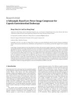
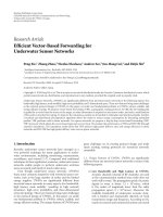
3.3. Schematic overview
The schematic overview of the proposed algorithm is given in
Figure 1. The idea is to alternately minimize the cost function
with respect to the common f and the PSFs h
i
. The flowchart
consists of two key steps. The first step performs recursive
image restoration to yield f
(i)
using f
(i−1)
, R
(i−1)
, and the new
data of the ith-channel. The second step performs blur iden-
tification using the conjugate gradient minimization to reach

f
(0)
= 0, R
(0)
= 0,
h
i
= impulse filter
i
= 0
i
= i +1
g
i
, h
i
, f
(i 1)
, R
(i 1)
ith-channel recursive
image restoration
f
(i)
, R
(i)
g
i
, h
i

, f
(i)
ith-channel
blur identification
h
i
No
i>K
Yes
No
Converge?
Yes
Restored image
f
(0)
= f
(K)
, R
(0)
= R
(K)
,
Figure 1: Schematic diagram of the proposed algorithm.
the optimal solution h
i
.LetK be the total number of chan-
nels, the inner loop of the procedure will run these two steps
alternately until data from all K channels have been com-
puted. Unlike recursive filtering in 1D adaptive filter design,
multichannel image restoration does not have hundreds of

measurements. Therefore, we propose to reuse the estimates
f
(0)
= f
(K)
, R
(0)
= R
(K)
from previous iteration in the
outer loop to reiterate the inner loop till the convergence is
reached.
Li Chen et al. 5
The contributions of the proposed technique, therefore,
include the following. (i) As opposed to other multichannel
restoration algorithms, it does not require all the data to be
available simultaneously as recursive filtering updates the es-
timate based on first-come-first-served basis. (ii) All the op-
erations of MRF for image-domain minimization are con-
ducted in the frequency domain through DFT, hence effi-
ciently reduce the computational cost. (iii) It incorporates
a forgetting factor to discard the old unreliable estimates,
hence achieving better convergence performance.
4. ISSUES ON PARAMETER SELECTION
4.1. Regularization parameters and operators
The regularization framework is instrumental in providing
satisfactory results in image restoration. Let e
(n)
denote the
residual error between f

(n)
in (11) and the original image f in
(1). In the DFT domain, e
(n)
is given by
e
(n)
(ω) =

f
(n)
(ω) −

f(ω)
=

n
i
=1
λ
n−i
H
H
i
(ω)n
i
(ω)

n
i

=1
λ
n−i



H
i
(ω)


2
+ α
i



C(ω)


2

−
f(ω)

n
i
=1
λ
n−i

α
i



C(ω)


2

n
i
=1
λ
n−i



H
i
(ω)


2
+ α
i



C(ω)



2

.
(19)
It can be observed that the error consists of two parts: the
noise and the image terms. The first part is the noise term,
which will be large for small H
i
(ω) if there is no regulariza-
tion term α
i
|

C(ω)|
2
.Thus,α
i
|

C
i
(ω)|
2
will reduce the impact
of noise term. However, this is at the cost of producing a
small bias to the actual image. In order to make e
(n)
as small

as possible, a reasonable compromise needs to be reached be-
tween these two terms by careful determination of regular-
ization parameter and operator. Previous work on the selec-
tion of the regularization parameter includes set theoretic ap-
proach and generalized cross-validation [19]. We follow the
idea of set theoretic in [19] to estimate the regularization pa-
rameters α
i
and β
i
:
α
i
=
ε
2
i
γ
2
≈
MNσ
2
i
c ∗ f
2
, β
i
=
ε
2

i
δ
2
i
≈
MNσ
2
i


d
i
∗ h
i


2
, (20)
where ε
i
, γ, δ
i
are the upper bounds related to the noise, im-
age, and PSF terms in (2). σ
2
i
is the noise variance in the ith-
channel, which can be estimated from the smooth regions of
the image. Equation (20) suggests a rule of thumb to choose
reasonable regularization parameters based on the noise, im-

age, and PSF conditions. In the experiments, the regulariza-
tion parameters α
i
and β
i
are initialized and remained con-
stant during the AM procedure. It is also possible to use the
estimated
σ
i
,

f,and

h to provide an order-of-magnitude esti-
mate for the regularization parameters [12, 14, 19]. The sim-
ulation results show that the algorithm is robust towards dif-
ferent regularization parameters so long as they fall within a
reasonable range.
As PSF is generally a low-pass filter, c should be taken as a
high-pass filter (or simply as an identity matrix C
= I), which
imposes smooth constraints on the images. The analysis on
the regularization operator d
i
is similar to c. In the appendix,
an analysis on how the regularization result of (10)isaffected
by the error in the PSFs is outlined.
4.2. Forgetting factor
The introduction of forgetting factor is centered on the ob-

servation that when the estimated image converges to the
original one, the identified blur will a pproach the actual PSF
in the alternating minimization scheme. It can be observed
from (10) that if the forgetting factor is 0
≤ λ<1, the
scheme will diminish older, less reliable estimated h
i
,andfa-
vor later, more updated estimate. Generally speaking, the for-
getting factor plays the role as an adaptive weight to ensure
that the data in the distant past are assigned less emphasis.
Even though the optimal value of the forgetting factor can
be derived theoretically using constrained optimization tech-
nique such as Lagrange multiplier method, this optimal value
is a function of the original image, PSF, and noise, of which
we have no prior knowledge. Therefore, it is tedious and im-
practical to estimate this optimal value during iterative min-
imization. It should also be noted from the experiments that
the proposed method will produce reasonable results so long
as the forgetting factor is within a reasonable range. There-
fore, estimation of exact optimal value is not required. In this
work, we let λ
= ζ
1/K
,whereζ is the memory attenuation
rate, K is the number of channels. For example, λ
= 0.3
1/K
means that the current channel has a weight of only 30% left
in its next iteration.

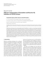
5. EXPERIMENTAL RESULTS
5.1. Multichannel blind restoration under
noisy conditions
The effectiveness of the proposed method is illustrated under
different blurring conditions. For performance evaluation,
peak signal-to-noise r atio (PSNR) is chosen as the objective
performance metric. In Figure 2(a), the original “Board” im-
age of size 256
× 256 is selected as the test image. The image
is blurred by four 5
× 5 Gaussian blurs:
h(i, j)
= a exp

−

i
2
+ j
2

2σ
2

, i, j = 0, ±1, ±2, (21)
corresponding to different values of σ
i
={2.0, 2.5, 3.0, 3.5},
where σ is the standard deviation of the Gaussian blur. The
parameter a is the normalization constant which ensures

the PSF coefficients sum up to 1. Further, the blurred im-
age is degraded under different noise levels to produce dif-
ferent SNR values
{30 dB, 33 dB, 36 dB, 40 dB}. Through this,
we can simulate four acquisition channels with variable blur-
ring functions and noise le vels, as shown in Figure 2(b).
The proposed MRF algorithm is run to perform
blind image restoration. All the degraded images are firstly
6 EURASIP Journal on Advances in Signal Processing
(a) (b)
(c) (d)
Figure 2: Multichannel blind image restoration results. (a) Original “Board” image. (b) A sampled blurred image out of the four degraded
images. (c) Restored image using the proposed MRF algorithm with identity regularization operator. (d) Restored image using the proposed
MRF algorithm with Laplacian regularization operator.
preprocessed using the edgetaper function in Matlab to en-
sure that the images are circularly symmetric. The forgetting
factor is taken as λ
= ζ
1/K
,whereζ = 0.05 and K = 4. The
regularization parameters are calculated according to (20),
while the regularization operators are simply taken as iden-
tity matrix or high-pass filter. The outer loop iteration num-
ber is set to 10, while the CGO iteration for blur identifica-
tion is 5.
The restored image using the proposed algorithm is
shown in Figures 2(c) and 2(d) . Figure 2(c) is the re-
stored image with identity regularization operator, while
Figure 2(d) is the restored image with Laplacian filter. It is
observed that the approach is effective in recovering detailed

information, as demonstrated by the clear numbers on the
board. The satisfactory subjective inspection of the image is
supported by objective performance measure as our method
offers a PSNR of 21.93 dB in Figure 2(c) and 22.43 dB in
Figure 2(d),comparedto12.46 dB for the degraded images.
Empirical results show that the proposed algorithm is not
sensitive to the exact choice of regularization operators so
long as they are reasonable. As the restored image with Lapla-
cian operator offers better PSNR value, we will use Laplacian
regularization operator for the next experiments.
5.2. Comparison with other multichannel
restoration methods
To further evaluate the effectiveness of our algorithm, we
compare the proposed algorithm with iterative multichan-
nel restoration methods, namely CGO-AM [12], TV-AM
[14], and Wiener filtering-alternating minimization (WF-
AM). The reason for choosing these methods for compara-
tive study is that these methods decompose the multichan-
nel blind deconvolution problem into two processes of im-
age restoration and blur identification, which are iteratively
optimized using alternating minimization. Their main dif-
ference lies in that the proposed method uses recursive filter-
ing to update the results. CGO-AM method adopts conjugate
gradient optimization (CGO) to minimize the image- and
blur-domain cost functions, while total variation (TV) and
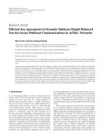
Li Chen et al. 7
(a) (b) (c)
(d) (e) (f)
Figure 3: Comparison of different restoration results in 30 dB noise environment. (a) Original “satellite” image. (b) One of the three de-
graded images. (c) Restored image using the proposed MRF algorithm. (d) Restored image using the CGO-AM algorithm. (e) Restored

image using the TV-AM algorithm. (f) Restored image using the WF-AM algorithm.
null space of blur are incorporated into the TV-AM scheme.
The parameter settings of CGO-AM and TV-AM are calcu-
lated according to [12, 14]. We have tried different parameter
assignments to determine the suitable setting for a ll meth-
ods. The approach of WF-AM is explained as follows. The
recursive filtering of image-domain cost function of the pro-
posed method is similar to Wiener filtering. Since blind im-
age restoration involves image restoration and blur identifi-
cation, we replace the ith-channel recursive image restora-
tion in Figure 1 by Wiener filtering. Conventional Wiener
filtering [20] is performed using f(w) = (H
i
(ω)
T
H
i
(ω)+
α
i
)
−1
H
i
(ω)
T
g
i
(ω), where α
i

is the power spectrum ratio of
the noise to the restored image. H
i
and g
i
are the PSF and de-
graded image in the ith-channel, respectively. This outlines
the WF-AM scheme to perform joint blur identification and
image restoration. The iteration number is set to 10 for all
methods.
The 256
× 256 “satellite image” shown in Figure 3(a) is
degraded by different blurs under different noisy conditions
(30 dB and 40 dB SNR noise). The proposed MRF, CGO-AM,
TV-AM, and WF-AM are applied to the blurred image in
Figure 3(b). The restored images are g iven in Figure 3(c)–
3(f) for 30 dB noisy conditions, where PSNR is tabulated
in Table 1 for 30 dB and 40 dB noisy conditions. On aver-
age, the proposed method yields 0.6 dB, 3.2 dB, and 3.8 dB
improvements over the CGO-AM, TV-AM, and WF-AM
methods, respectively. By comparing the restored images
shown in Figures 3(c)–3(f), it is clear that our approach is su-
perior in preserving details of satellite. This is supported by
objective performance measure as our method offers PSNR
of 29.41 dB, as opposed to 28.70 dB, 26.10 dB, and 25.85 dB
by the CGO-AM, TV-AM, and WF-AM methods, respec-
tively. The proposed method utilizes recursive updating tech-
nique, coupled with forgetting term to prioritize newer, more
recent estimates. In contrast, the error in previous estimate
will be propagated in the CGO-AM method. On the other

hand, the WF-AM method inherits no information from the
older estimate as each channel restores the image indepen-
dently. Further, the TV-AM method requires all the PSFs to
be coprime. As this assumption is not satisfied in the experi-
ment, the TV-AM method fails to provide satisfactor y results.
The overall complexity is a combination of the conver-
gence rate and the time complexity for each single iteration.
The proposed method, generally, has faster convergence rate
with moderate single-iteration complexity. To illustrate this,
we try to compare the computational time of these meth-
ods using the same platform. The simulation environments
of these methods are Windows XP, MATLAB 6.5, CPU P4-
2.4 GHz, and 512 M RAM. It takes 64 seconds in terms of the
running time, as compared to 89 seconds, 179 seconds, and
55 seconds by the CGO-AM, TV-AM, and WF-AM methods,
respectively. T he reason that the proposed method is faster
8 EURASIP Journal on Advances in Signal Processing
Table 1: Comparison of different restoration algorithms.
PSF Gaussian 7 ×7, σ
i
={2.5, 3.0, 3.5}
Time
Noise level 30 dB 40 dB
Proposed MRF 28.58 dB 29.41 dB 64 s
CGO-AM 27.96 dB 28.70 dB 89 s
TV-AM 25.42 dB 26.10 dB 179 s
WF-AM 24.54 dB 25.85 dB 55 s
0 10203040506070
26
26.5

27
27.5
28
28.5
29
29.5
30
Iterations
PSNR
0.6
0.8
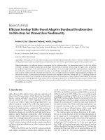
1
Figure 4: The profile of PSNR versus the number of iterations with
different forgetting parameters λ
= ζ
1/5
,whereζ ={0.6, 0.8, 1.0}.
than the CGO-AM and TV-AM methods is due to efficient
recursive updating of the images.
5.3. Impact of forgetting factor
To study the impact of forgetting factor experimentally, the
proposed MRF algorithm is run with different forgetting fac-
tors. The 256
×256 “Lena” image is degraded by 7 ×7Gaus-
sian blurs with σ
i
={2.0, 2.3, 2.6, 2.9, 3.2}. The regulariza-
tion operators are standard Laplacian high-pass filter. Based
on the 5 observed degraded images, the proposed MRF al-
gorithm is repeated, but with different forgetting parameters

λ
= ζ
1/5
,whereζ ={0.6, 0.8, 1.0}. The outer loop iteration
number is set to 14. As there are 5 channels, each inner loop
iteration will update the image 5 times. The overall iteration
of the recursive filtering is 70. The profile of PSNR versus the
number of iterations is plotted in Figure 4. It is observed that
the curve tends to become flatter when the forgetting factor
becomes larger. This indicates slower convergence rate. λ
= 1
means infinite memory as the effect of past data is not atten-
uated and this gives rise to slow convergence r ate.
In this work, we simply use λ
= ζ
1/K
to show that the al-
gorithm can have different convergence rate for different for-
getting factors. Good results can be obtained if we terminate
the algorithm when the relative change in consecutive itera-
tion is less than a predefined threshold. Further study on the
effect of forgetting factor is interesting and we hope that this
work will stimulate further investigation.
6. CONCLUSION
This paper proposes an iterative blind multichannel image
restoration algorithm based on recursive filtering. The esti-
mated image is recursively updated from its previous esti-
mate using a regularization framework. It incorporates a for-
getting factor to discard the old unreliable estimates, hence
achieving better convergence performance. The proposed

computational structure is novel and it makes the overall
computation efficient, especially in the area of multichannel
reconstruction. This allows the new method to be adopted
readily in real-life applications. Experimental results show
thatitiseffective in performing blind multichannel blind
restoration.
APPENDIX
In this appendix, the error bound for the regularization
scheme is studied. The error bound for the least squares so-
lution to the overdetermined and underdetermined systems
Ax
= b is presented in [21]. To examine how the regulariza-
tion solution is affected by the changes in A and b, the reg-
ularized solution to the underdetermined/overdetermined
systems Ax
= b is investigated.
Proposition 1. Suppose A
∈ R
m×n
, δA ∈ R
m×n
, 0 = b ∈
R
m
, δb ∈ R
m
, 0 <α∈ R,andrank(A) = m<n.Letε =
max{ε
A
, ε

b
},whereε
A
=δA
2
/A
2
and ε
b
=δb
2
/b
2
.
If x and
x are the regularization solutions that satisfy
x
=

A
T
A + αI

−1
A
T
b = A
T

AA

T
+ αI

−1
b,
x =

(A + δA)
T
(A + δA)+αI

−1
(A + δA)
T
(b + δb),
(A.1)
then
x − x
2
x
2
≤ ε

κ
2
(A)+
A
2
2
√

α

1+
b
2
A
2
x
2

+ O

ε
2

.
(A.2)
Proof. Let E and q be defined by δA/ε and δb/ε.Itfollows
that the solution x(t)to

(A + tE)
T
(A + tE)+αI

x(t) = (A + tE)
T
(b + tq)(A.3)
is continuously differentiable for all t
∈ [0, ∞).
Define P

1
= A
T
A + αI and P
2
= AA
T
+ αI,weobtain
P
−1
1
A
T
= A
T
P
−1
2
,
x
2
=


A
T
P
−1
2
b



2
≥ σ
m


P
−1
2
b


2
,


P
−1
1


2
=
1
α
,


P

−1
2


2
=
1

σ
2
m
+ α

,


P
−1
1
A
T


2
= max
i
σ
i

σ

2
i
+ α

≤
1/

2
√
α

,
(A.4)
where σ
i
is the singular value of A and σ
1
≥ σ
2
≥···≥σ
m
> 0.
Li Chen et al. 9
By differentiating (A.3)withrespecttot and setting t = 0
in the result, we obtain
˙
x(0)
= P
−1
1

A
T
(q − Ex)+αP
−1
1
E
T
P
−1
2
b. (A.5)
Since x
= x(0), x = x(ε), the error upper bound is given by
x − x
2
x
2
= ε

˙
x(0)

2
x
2
+ O

ε
2


≤
ε


A
2


P
−1
1
A
T


2


q
2
A
2
x
2
+
E
2
A
2


+
α
σ
m
A
2


P
−1
1


2


E
T


2
A
2

+ O

ε
2

≤

ε
A
κ
2
(A)+
A
2
2
√
α

ε
A
+ ε
b
b
2
A
2
x
2

+ O

ε
2

(A.6)
thereby establishing (A.2).
The extension of error bound to SIMO system in (10)

when C
= I is straightforward by setting
A
=
⎡
⎢
⎢
⎢
⎢
⎢
⎣
λ
n
H
1
λ
n−1
H
2
.
.
.
H
n
⎤
⎥
⎥
⎥
⎥
⎥

⎦
, δA =
⎡
⎢
⎢
⎢
⎢
⎢
⎣
λ
n
δH
1
λ
n−1
δH
2
.
.
.
δH
n
⎤
⎥
⎥
⎥
⎥
⎥
⎦
,

b
=
⎡
⎢
⎢
⎢
⎢
⎢
⎣
λ
n
g
1
λ
n−1
g
2
.
.
.
g
n
⎤
⎥
⎥
⎥
⎥
⎥
⎦
, δb =

⎡
⎢
⎢
⎢
⎢
⎢
⎣
λ
n
δg
1
λ
n−1
δg
2
.
.
.
δg
n
⎤
⎥
⎥
⎥
⎥
⎥
⎦
,
x
= f, α =

n

i=1
λ
n−i
α
i
.
(A.7)
In this case, the regularization operator is taken as impulse
filter to simplify the analysis. Suppose that the estimated H
i
converges to the actual PSF during the iterative MRF scheme,
we will have δH
n
≤ ··· ≤ δH
2
≤ δH
1
. Therefore, δA
in (A.7) will be reduced as the forgetting factor assigns less
weight to larger error of δH
i
. In this sense, the upper bound
error will be reduced progressively.
REFERENCES
[1] D. Kundur and D. Hatzinakos, “Blind image deconvolution,”
IEEE Signal Processing Magazine, vol. 13, no. 3, pp. 43–64,
1996.
[2] B. R. Hunt and O. Kuebler, “Karhunen-Loeve multispectral

image restoration, part I: theory,” IEEE Transactions on Acous-
tics, Speech, and Signal Processing, vol. 32, no. 3, pp. 592–600,
1984.
[3] S. U. P illai and B. Liang, “Blind image restoration using a ro-
bust GCD approach,” IEEE Transactions on Image Processing,
vol. 8, no. 2, pp. 295–301, 1999.
[4] G. Harikumar and Y. Bresler, “Perfect blind restoration of
images blurred by multiple filters: theory and efficient algo-
rithms,” IEEE Transactions on Image Processing, vol. 8, no. 2,
pp. 202–219, 1999.
[5] G. B. Giannakis and R. W. Heath Jr., “Blind identification of
multichannel FIR blurs and perfect image restoration,” IEEE
Transactions on Image Processing, vol. 9, no. 11, pp. 1877–1896,
2000.
[6] H T. Pai and A. C. Bovik, “On eigenstructure-based direct
multichannel blind image restoration,” IEEE Transactions on
Image Processing, vol. 10, no. 10, pp. 1434–1446, 2001.
[7] N. P. Galatsanos, A. K. Katsaggelos, R. T. Chin, and A. D.
Hillery, “Least squares restoration of multichannel images,”
IEEE Transactions on Signal Processing, vol. 39, no. 10, pp.
2222–2236, 1991.
[8] M. G. Kang and A. K. Katsaggelos, “Simultaneous multichan-
nel image restoration and estimation of the regularization pa-
rameters,” IEEE Transactions on Image Processing, vol. 6, no. 5,
pp. 774–778, 1997.
[9] Y. Yang, N. P. Galatsanos, and H. Stark, “Projection-based
blind deconvolution,” Journal of the Optical Society of America
A, vol. 11, no. 9, pp. 2401–2409, 1994.
[10] Y L. You and M. Kaveh, “Regularization approach to joint
blur identification and image restoration,” IEEE Transactions

on Image Processing, vol. 5, no. 3, pp. 416–428, 1996.
[11] T. F. Chan and C. K. Wong, “Convergence of the alternating
minimization algorithm for blind deconvolution,” Linear Al-
gebra and Its Applications, vol. 316, no. 1–3, pp. 259–285, 2000.
[12] T. W. S. Chow, X D. Li, and K T. Ng, “Double-regularization
approach for blind restoration of multichannel imagery,” IEEE
Transactions on Circuits and Systems I: Fundamental Theory
and Applications, vol. 48, no. 9, pp. 1075–1085, 2001.
[13] R. Molina, J. Mateos, A. K. Katsaggelos, and M. Vega,
“Bayesian multichannel image restoration using compound
Gauss-Markov random fields,” IEEE Transactions on Image
Processing, vol. 12, no. 12, pp. 1642–1654, 2003.
[14] F. Sroubek and J. Flusser, “Multichannel blind iterative image
restoration,” IEEE Transactions on Image Processing, vol. 12,
no. 9, pp. 1094–1106, 2003.
[15] G. Panci, P. Campisi, S. Colonnese, and G. Scarano, “Multi-
channel blind image deconvolution using the Bussgang algo-
rithm: spatial and multiresolution approaches,” IEEE Transac-
tions on Image Processing, vol. 12, no. 11, pp. 1324–1337, 2003.
[16] S. Haykin, Adaptive Filter Theory, Prentice-Hall, Upper Saddle
River, NJ, USA, 4th edition, 2002.
[17] L. Chen and K H. Yap, “A soft double regularization approach
to parametric blind image deconvolution,” IEEE Transactions
on Image Processing, vol. 14, no. 5, pp. 624–633, 2005.
[18] L. Chen and K H. Yap, “Efficient discrete s patial techniques
for blur support identification in blind image deconvolution,”
IEEE Transactions on Signal Processing, vol. 54, no. 4, pp. 1557–
1562, 2006.
[19] N. P. Galatsanos and A. K. Katsaggelos, “Methods for choosing
the regularization parameter and estimating the noise variance

in image restoration and their relation,” IEEE Transactions on
Image Processing, vol. 1, no. 3, pp. 322–336, 1992.
[20] H. C. Andrews and B. R. Hunt, Digital Image Restoration,
Prentice-Hall, Upper Saddle River, NJ, USA, 1977.
[21] G. H. Golub and C. F. Van Loan, Matrix Computations,John
Hopkins University Press, New York. NY, USA, 3rd edition,
1996.
10 EURASIP Journal on Advances in Signal Processing
Li Chen received B.Eng. degree in indus-
trial automation from Wuhan University of
Technology, Wuhan, China, in 1999, the
M.Eng. degree in control theory from
Huazhong University of Science and Tech-
nology, Wuhan, China, in 2002, and the
Ph.D. degree in information engineering
from Nanyang technological University,
Singapore, in 2006. He is currently a Re-
search Associate at Nanyang Technological
University, Singapore. His research interests include image process-
ing, statistical pattern recognition, and computer vision.
Kim-Hui Yap received the B.Eng. and Ph.D.
degrees in electrical engineering from the
University of Sydney, Sydney, Australia, in
1998 and 2002, respectively. Currently, he is
a Faculty Member at Nanyang Technolog-
ical University, Singapore. His research in-
terests include adaptive image processing,
computational intelligence, and multimedia
signal processing. He has more than thirty
publications in various international jour-

nals, conference proceedings, and book chapters. He is also the Ed-
itor of a book entitled Intelligent Multimedia Processing with Soft
Computing by Springer-Verlag in 2005.
Yu He received B.Eng. degree in precision
instrument and optoelectronics engineer-
ing from Tianjin University, Tianjin, China,
in 2002. After that he worked as a Research
and Develepment Engineer in the SAM-
SUNG Electronic Co. Ltd. (color TV) for
two years. He is currently a Ph.D. student
at Nanyang Technological University, Sin-
gapore. His research interests include image
and video deconvolution, and super resolu-
tion.