Báo cáo hóa học: "Research Article A Novel Distributed Privacy Paradigm for Visual Sensor Networks Based on Sharing Dynamical Systems" pptx

Hindawi Publishing Corporation
EURASIP Journal on Advances in Signal Processing
Volume 2007, Article ID 21646, 17 pages
doi:10.1155/2007/21646

Research Article
A Novel Distributed Privacy Paradigm for Visual Sensor
Networks Based on Sharing Dynamical Systems
William Luh, Deepa Kundur, and Takis Zourntos
Department of Electrical and Computer Engineering, 214 Zachry Engineering Center, Texas A&M University, College Station,
TX 77843-3128, USA
Received 5 January 2006; Revised 29 April 2006; Accepted 30 April 2006
Recommended by Chun-Shien Lu
Visual sensor networks (VSNs) provide surveillance images/video which must be protected from eavesdropping and tampering en
route to the base station. In the spirit of sensor networks, we propose a novel paradigm for securing privacy and confidentiality
in a distributed manner. Our paradigm is based on the control of dynamical systems, which we show is well suited for VSNs due
to its low complexity in terms of processing and communication, while achieving robustness to both unintentional noise and
intentional attacks as long as a small subset of nodes are affected. We also present a low complexity algorithm called TANGRAM
to demonstrate the feasibility of applying our novel paradigm to VSNs. We present and discuss simulation results of TANGRAM.
Copyright © 2007 Hindawi Publishing Corporation. All rights reserved.

1.

INTRODUCTION

Visual data is an integral part of the interface between humans and their environment. Visual data in the form of images and video can be used to enhance a human operator’s
ability to reliably make crucial decisions in the face of alerts
provided by sensing mechanisms. For example, in a combat field, a sensor network can be deployed to sense temperature, toxins, vibrations/movement, and so forth. To reliably
assess whether a change in the sensed phenomena is due
to enemy infiltration or natural environmental and fauna
causes, it is useful to obtain additional side information in

the form of an image. As another example, in health care
facilities [1, 2], one may measure a patient’s vital statistics,
such as heart rate, using sensors. When such measured statistics indicate that the patient is in imminent danger, visual
side information may quickly determine whether the measurements are valid or caused by misplaced or malfunctioning sensors. Following this motivation, acquisition of visual
data in sensor networks can be used to enhance the quality
of service in surveillance applications in which a human operator interfaces at the sink of the network [3]. Such sensor
networks are called visual sensor networks (VSNs) or often
multimedia sensor networks [4]. The emergence of low-cost
portable off-the-shelf sensor devices has thrust forward the
development of VSN architectures, systems, and testbeds [1–
3, 5–12].

Acquisition and processing of visual data in sensor networks come at a cost. First, visual data in the form of images
or video require larger storage and transmission resources
than do traditional scalar data such as temperature or heart
rate. These resource requirements are further bloated when
every sensor is equipped to acquire and process images and
video. Furthermore, image processing requires more power
to process than conventional scalar data, and hence VSNs
may not meet the resource constraints placed upon traditional scalar-data-based sensor networks. This suggests that
visual data should be acquired and processed judiciously,
perhaps by one or two cameras within a confined area.
However as we consider in this paper, from the perspective
of resilience to physical and electronic attack, dense VSNs
demonstrate potential for security and surveillance applications.
Visual data may be intercepted by illicit parties for use
not originally intended. For example, in a military scenario,
interception of surveillance images can be used by an enemy
to learn and counter the efforts of a mission. In a health-care
scenario, interception of images by outsiders compromises

patient privacy rights. Therefore a means to protect these images needs to be built into VSNs. In order to combat physical
attacks, electronic means are often employed in addition to
more robust ad hoc networking architectures. For example,
the “one camera” architecture suggested above is vulnerable
to physical attacks such as unlawful interception, tampering,


2

EURASIP Journal on Advances in Signal Processing

or capture of entities in the network. Instead of preventing
such actions, it is more feasible to engineer information security mechanisms to deny illicit parties access to the semantic
content of visual data.
Traditionally, to deny third parties access to content, encryption is employed [13]. However, recently it has been
noted that the use of these powerful cryptosystems on visual data further exacerbates processing power (resource)
requirements as mentioned above [14–16]. Measures have
been taken to trade off security with processing complexity,
and in this paper we follow this philosophy.
In the spirit of sensor networks, we opt for a densely distributed architecture in which every sensor is equipped with
a camera for visual acquisition, as well as some simple image processing capabilities. It is not difficult to envision that
physical security based on a distributed infrastructure shares
all the same advantages as those in which sensor network research pioneers were drawn to. The principle of redundancy
compensates for sensor failure either due to natural (i.e., battery failure, noise in the environment, or sensor hardware) or
malicious causes. From a physical security standpoint, distribution offers safeguard against illicit capture of a few sensor
nodes and its cryptographic keys stored on-board [17, 18],
which we term node capture. Attackers are hence forced to
capture all nodes or intercept all relevant node communique
in order to access semantic information. In this paper, we
propose a general paradigm for distributing security in a visual sensor network.

1.1. Scope and contribution
We focus, in this paper, on presenting a novel distributed
approach to protect dense VSNs against eavesdropping attacks. Other security issues including authentication, message freshness and replay, key management, physical and actuation attacks, and common denial-of-service attacks are,
in part, considered by existing sensor network security literature and are beyond the scope of the paper.
In [19], security for the IP-based video surveillance problem is considered. In this paper we consider a distributed
security scheme for VSNs in which camera nodes work together. We consider a VSN, which we define to be a collection
of sensor nodes each having image acquisition and processing capabilities. Within a VSN, a cluster of nodes is defined
to be a subset of N nodes that are recording or capturing the
same scene at approximately the same camera orientation. A
security goal of each node in a cluster is to send partial visual
information, which we call shares to a base station or multiple base stations, such that
(1) the base station(s) can reconstruct (or decrypt) an approximation of the scene being recorded by the cluster
when t + 1 or more shares are available;
(2) interception of t or fewer shares will not reveal the
scene being recorded.
Secret sharing, popularized by Shamir [18], is the process
by which a trusted central authority called the dealer creates
and securely distributes N shares to N participants, such that

only certain subsets of participants can recover a secret key
K by amalgamating their shares. Our problem is similar to
secret sharing, except for the following differences:
(1) traditional secret sharing requires a trusted central authority to create the shares and distribute them securely; in our distributed VSN problem, a different
share is created by each node of a cluster (with some
minor coordination to guarantee robust recovery);
(2) we allow for t or fewer nodes to be captured, thus revealing any secret keys;
(3) we allow for t or fewer shares to be corrupted or tampered with.
We now point out other existing secret sharing works,
and show how our work differs. In visual secret sharing (VSS)
[20–23], the goal is similar; a dealer creates N transparencies

and securely distributes them to N participants. If a subset of
transparencies are overlaid upon one another, the secret image is revealed—this is the decryption process. In most VSS
schemes, the decryption process (i.e., overlaying transparencies) has lower complexity than either creating the shares or
transmitting/storing them. This is due to the fact that extra
information must be embedded into the transparencies in
order to support such trivial decryption. In sensor networks,
this is not favorable; instead the opposite role is favored, being that complexity is lower at the encrypting end (node
end), and higher at the decrypting end (base station end)
[24]. Of course VSS also suffers from the need for a trusted
central authority as does secret sharing. Next, we point out a
distributed encryption scheme that does not require a trusted
central authority based on the RSA public-key cryptosystem
[25, 26]. One draw-back of [25, 26] is that this public-key
cryptography scheme was not developed for sensor networks
(but rather for fault-tolerant distributed systems), hence the
complexity at the node end is much higher. In addition, the
method is not always immune to node capture, particularly
if the so-called source node is captured, key information can
be used to reveal the secret.
To this end, this paper offers a general paradigm for
creating shares in a VSN, and hence many algorithms can
be created based on the same principles. The use of dynamic system theory for this purpose is novel and, as
we demonstrate, provides the following attractive characteristics: (a) dynamism and evolution to exploit the distributed and collaborative nature of VSNs for share generation, (b) robustness to compensate for sensor error and malicious tampering, (c) obfuscation in order to provide image/video scrambling with a more competitive compromise
between security and practicality for VSNs, and (d) flexibility and simplicity for lightweight implementation. The dynamic system approach allows the creative incorporation of
the many competing VSN objectives of robustness, security and practicality into a framework with well-developed
mathematical background based on Lyapunov theory. This
has the advantage of producing a solution that is distributed and lower complexity and hence most appropriate for VSNs in comparison to the existing methods surveyed above. We analyze our proposed technique, called


William Luh et al.

TANGRAM, to demonstrate its potential performance and
practicality.
Finally, we note that our paradigm is geared towards visual data, or any kind of data whose semantics are not destroyed by small perturbations. The inherent redundant nature of visual data offers both pros and cons. On the one
hand, visual redundancy offers resiliency against errors. On
the other hand, visual redundancy translates into higher
communication and storage costs. Hence a tradeoff between
robustness and compression is also considered in this paper.
This paper is separated into three parts. In Section 2, the
general paradigm is presented. Within this section we formulate the problem, introduce notations and definitions, and finally present the general architecture and guiding principles
used to design a solution. In Section 3, we present an algorithm using our paradigm. In Section 4, we present simulation results to verify visual security.
2.

GENERAL PARADIGM

In this section we develop the general paradigm.1 First we
formally present the problem and assumptions. Next we define basic elements used in the framework, and finally we
present the paradigm.

3
S ⊆ {I0 , I1 , . . . , IN −1 }, and subset of sensor nodes3 T ⊆ {0, 1,
. . . , N − 1} corresponding to S
(1) if the cardinality of S is greater than t, that is, |S| > t,
then a visual approximation of Ir can be derived from
S;
(2) if |S| ≤ t, then a visual approximation of Ir cannot be
derived from S alone;
(3) if the sensor nodes of T with |T | ≤ t are physically
captured and removed from the network, any statically
stored information4 on these nodes along with the corresponding shares in S will not help the attacker in deriving a visual approximation of Ir ;
(4) key management in the form of rekeying or key updates is not necessary to deal with the particular issues

addressed in this paper.
We will define the quantitative notion of visual approximation in the coming subsection. Also we note that although
existing secret sharing algorithms can be adjusted to satisfy
point 3 through rekeying or key updating, our paradigm
does not explicitly require key management leading to a more
practical solution for distributed VSNs.
2.1.2. Assumptions
We now impose the following assumptions on the attacker.

2.1. Problem formulation
Suppose a collection of N sensor nodes equipped with image acquisition and processing capabilities is deployed in
close physical proximity such that they all capture the same
scene. To quantify this statement, let {I0 , I1 , . . . , IN −1 } represent the N grayscale images captured by the N nodes.2 Here
Ii , 0 ≤ i ≤ N − 1 are m × n matrices containing integer
values in the set {0, 1, . . . , 255}. Assume that these N images are noisy versions of a representative image Ir , such that
Ii = Ir + nr , where nr is a random matrix of integers based on
some distribution with zero-mean and small variance. This
assumption allows us to approximate the different sensor acquisitions as the same image, that is, Ii ≈ Ir , which will simplify the computations. We will justify this assumption soon
in the coming section.
We also assume that the VSN is capable of pairwise (between two neighboring nodes) and individual (between node
and base station) key distributions. In addition, each node is
capable of communications to neighboring nodes and to the
base station (possibly via multihop networking).

(1) The attacker has limited ability to employ physical attacks on the observation area. Specifically, the attacker
cannot deploy his own cameras to capture the same
scene as the VSN nodes nor can he physically attack
the observation area such as block the scene.5 In addition, the attacker can only physically capture and remove nodes from the network, but cannot wiretap a
node and eavesdrop on all activities on-board a sensor
node.

(2) The attacker can only intercept or tamper the shares of
a subset of nodes of cardinality ≤ t.
(3) The attacker is less likely to intercept communication between nodes without being detected due to the
nodes being in close proximity; the attacker is more
likely to intercept communication between nodes and
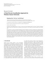
the base station(s). See Figure 1.
We impose the following assumptions on the sensor
nodes.
(1) The VSN is aware when a node is removed from the
network, and will stop communicating with the rogue
node.
(2) Every node can perform the duties of any other node.
Hence when a node dies, the nodes within a cluster
can reorganize their logistics. In addition, nodes are

2.1.1. Goals of this paradigm
The goal is for each sensor node i to encrypt its image Ii , resulting in the share Ii , such that for some subset of shares
3
1

In this paper we generalize the paradigm previously developed in [27],
hence encompassing a broader class of algorithms.
2 Color images can be treated in the same manner by defining accompanying color planes dependent on formats such as RGB, HSV, YCbCr, and so
forth.

In this paper, we denote N nodes by giving them unique integer identifiers
starting with 0.
4 By statically stored, we mean keys, codebooks, and so forth. Any values
created from computation would not be statically stored.
5 Physical actuation attacks considered in, for example, [28] are beyond the

scope of this work.


4

EURASIP Journal on Advances in Signal Processing
Common scene

replenished so that an area of observation is never left
starved for nodes.
(3) We assume that the nodes are capable of repositioning collectively (i.e., rotating panoramically) to capture different scenes in order to avoid the message resend attack [29].

Node
0

¡¡¡

Node
1

Node
N  1
Cluster

2.2. Preliminaries

Attack most likely en route to base station

In this section we define the basic elements used in our
paradigm. First we define an image space by converting an

image matrix Ii into a (m · n) × 1 column vector xi , via a
column-wise raster scan as shown in (1).
⎛

⎞
x1,1
x1,2 · · · x1,n−1
x1,n
⎜
⎟
⎜
⎟
⎜ x2,1
x2,2 · · · x2,n−1
x2,n ⎟
⎜
⎟
⎜
⎟
⎜ .
.
.
. ⎟,
..
Ii = ⎜ .
.
.
. ⎟
.
.

.
. ⎟
⎜ .
⎜
⎟
⎜x
⎟
⎜ m−1,1 xm−1,2 · · · xm−1,n−1 xm−1,n ⎟
⎝
⎠
xm,1 xm,2 · · · xm,n−1 xm,n

Base station

Base station

Base station

Figure 1: Communication scheme, layout of a cluster, and the most
common point of attack.

Every state outside is
perceptually dissimilar to xi

T

xi = x1,1 x2,1 · · · xm,1 x1,2 x2,2 · · · xm,2 · · · xm,n .
(1)
The collection of all (m · n) × 1 column vectors constitutes
our image space, and each column vector is called a state.

We note that although we defined an image to take on integer values in the range 0 to 255, the image space includes all
(m · n) × 1 column vectors with real elements. This collection
along with the usual operators is a vector space over the real
field.
Our notion of visual approximation is based on the norm
of a vector.6 The norm of a vector xi is the l2 –norm denoted by xi . To quantify visual similarity or dissimilarity
for practical use, two variables ρ0 ≤ ρ1 are chosen as a function of the (image) state xi in question, such that the annulus
centered about xi , as given in (2), completely defines the visual similarity and dissimilarity:
Axi = x : ρ0 ≤ x − xi ≤ ρ1 .

(2)

The complement of the annulus can be separated into two
regions: the region enclosed by the annulus is called the similar region, where the states in here share the semantics of
xi ; the region outside the annulus is called the dissimilar region, where the semantics of xi cannot be visually deduced
from states in here. The annulus itself defines a fuzzy region, which accounts for differences in individual perception.
Figure 2 illustrates the partitioning of the image space into
6

We note that although this notion does not model the human visual system accurately, it is used often for reasons of simplicity in MPEG encoding, for example block matching [30].

xi
p0
p1

Every state in this region is
perceptually similar to xi

“Fuzzy” region

Figure 2: Separation of image space into perceptual similar, dissimilar, and fuzzy regions.

similar, dissimilar, and fuzzy regions. It is clear that the variables ρ0 ≤ ρ1 depend on the human visual system, and hence
is application-dependent.
2.3.

Architecture and principles

Suppose that every sensor node records the representative image Ir (i.e., the common scene), which corresponds
with the representative state x. The central idea behind our
paradigm is that we design a discrete-time dynamical system
such that each node has an access to only a certain part of
this dynamical system and not to its entirety. Identifiers 0 to
N − 1 are assigned to each of the N nodes. A node with identifier k is then responsible for applying a control to move the
state at time k of the dynamical system closer to the desired
x. The node’s control is the node’s share. Since an attacker
who intercepts a subset of shares and/or physically captures


William Luh et al.

5
Require: Initial state x0 loaded into node 0 and partial system fi for each node i;
all nodes capture common scene represented by x
Ensure: Shares ui , 0 ≤ i ≤ N − 1
(1) for k = 0 to N − 1 do
(2) {Each iteration is performed by a different node, i.e., node k}
(3) if k = 0 then
(4)
Receive ek−1,k from node k − 1

(5)
xk ⇐ DKk−1,k ek−1,k {Decrypt with pair-wise key shared with node k − 1}
(6) end if
(7) uk ⇐ gk (xk , x) {To be designed to drive states to x}
(8) if k = N − 1 then
(9)
xk+1 ⇐ fk xk , uk
(10)
ek,k+1 ⇐ EKk,k+1 xk+1 {Encrypt with pair-wise key shared with k + 1}
(11)
Destroy xk+1 {So if this node is captured, attacker does not have this}
(12)
Send ek,k+1 to node k + 1
(13) end if
(14) if k = 0 then
(15)
Destroy xk {So if this node is captured, attacker does not have this}
(16) end if
(17) Send uk to the base station {This is node k’s share}
(18) end for
Algorithm 1: Distributed encryption for VSN.

a subset of nodes only knows part of the dynamical system,7
the attacker cannot drive this partial dynamical system to the
secret x. In Section 2.4, we will discuss the motivation for using this paradigm.
From the dynamical systems literature, let Σ p be a userdesigned plant that is described by a state equation (discretetime difference equation) as in (3):
Σ p : xk+1 = fk xk , uk , wk .

(3)

Here, the vectors denoted by xk are called states, the vectors
denoted by uk are external controls/inputs, and wk is a random vector noise term. Every node agrees ahead of time on
a starting node, also called the source node [25], which contains a randomly generated initial state x0 (i.e., independent
of Ir ), either through preprogramming the node hardware,
or some key distribution protocol.
Next we ensure that every node is endowed with only part
of the plant or that there is a random component of which
only one node is aware. For example, if the system is timevarying, each node is endowed with a unique set of the parameters corresponding to each time instance. To be more
precise, let the nodes be numbered 0 to N − 1. Then node i
is endowed with fi , and for node i = j, fi = f j ; that is each
node only knows part of the system. Finally each node runs
an optimization algorithm whose goal is to drive any given
state to x. The pseudocode is presented in the table entitled
7

This does not violate Kerckhoff ’s principle [13], which states that the security of a system should only reside in the key, while the system can be
known. In practice, we can publish the system to be used, but keep secret
the system parameters, which can be regarded as keys.

Algorithm 1. Here we define ei, j to be the encrypted state,
which is created by node i and sent to node j.
In Algorithm 1, each iteration of the loop reflects the activity of one particular node, namely the node associated
with the loop index k. We see that the source node 0 starts
off the algorithm by applying a function g0 (line 7—to be
designed) on the initial state x0 and the representative state
x—this is the external input or the so-called control to the
plant Σ p . This control is then applied to the plant (line 9),
and the result is encrypted using a pair-wise key shared with
node 1 (line 10), and sent to node 1 (line 12). Continuing
with the remaining iterations of the loop, each node hereafter receives an encrypted state (line 4) from the previous

node, which is able to decrypt with its pair-wise key shared
with the previous node (line 5). The node then uses this state
to derive a new control (line 7), which drives the states closer
to the desired representative state x. The new state generated
by this control (line 9) is then encrypted with the pair-wise
key shared with the next node (line 10) and sent to the next
node (line 12). The controls generated by each node constitute the set of shares, which are sent to the base station(s).
An overview of the communication scheme is depicted in
Figure 1. From an overall system perspective, the nodes can
be considered to cooperate to drive an initial state to the desired representative state x by applying a control (which is the
node’s share) to the system via the state created by a previous
node, and then relaying the updated state to the next node.
Since the controls drive the plant to x, the decryption algorithm is straight-forward as shown in Algorithm 2.
In order to decrypt, all the controls (or shares) and the
entire plant/system must be known. Hence an attacker is
forced to intercept all shares, or capture all nodes. Figure 3(a)
illustrates how the initial state is driven to the desired representative state x. When a control is applied to a state, the


6

EURASIP Journal on Advances in Signal Processing
Require: All shares ui , 0 ≤ i ≤ N − 1 received by base station(s),
and base station(s) have all fi , 0 ≤ i ≤ N − 1 and x0
Ensure: xN = x
(1) {Loop performed by a central unit at the base station}
(2) for k = 0 to N − 1 do
(3) xk+1 ⇐ fk xk , uk
(4) end for
Algorithm 2: Decryption at base station(s) for VSN.

dynamical system is moved to a new state. Controls are applied successively to the dynamical system to drive the state
to x and hence reconstruct the representative image Ir .
Finally, each iteration in Algorithm 1 can be thought of as
a round which adds confusion, hence Algorithm 1 mimics an
iterated block cipher [31] with each round being performed
by a single different node using a different key.
2.4. Motivation for this paradigm
There are many reasons why a dynamical systems approach
is chosen for this problem. Such theory is well developed to
handle external disturbances. For our problem, this is useful to ensure that image decryption is robust to natural (unintentional) system disturbances such as hardware noise, or
intentional tampering. If we assume that the disturbance wi
is additive and constrained, for example bounded such that
wi < C, then control laws can be designed such that the
trajectory stays within some region around the desired representative state x as illustrated in Figure 3(b). If the ball
around x has radius ρ0 or less, where ρ0 is the variable accounting for perceptual similarity from Section 2.2, then decryption will still result in a good visual approximation of the
desired image.
2.5. Extensions
This robustness allows for some additional advantages. The
number of pair-wise keys that each sensor node carries to run
the proposed algorithm is always 2 (i.e., O(1)) regardless of
the number of nodes in a cluster. This is because node k only
needs to receive the previous state from node k − 1 and must
send its current state to node k + 1 requiring communication only among these nodes. This is a memory advantage
because, in contrast to the sharing scheme presented in [25],
√
the number of key fragments per node is O( N), where N is
the number of nodes. Finally, if each node is regarded as a
vertex, and the communication between nodes is a directed
edge, then the VSN is a directed graph. The number of fanouts, or outdegree of each node in our scheme is exactly 2

(one for transmitting to the next node, and one for transmitting to the base station(s)) regardless of the number of
nodes in the cluster (i.e., O(1)). However, the outdegree per
√
node in [25] is again O( N). Also, the unidirectional nature
of the internode communication in our paradigm promotes
an optical sensor network architecture [32], which has been
shown to be energy-efficient for communicating multimedia
through free space [33].

3.

TANGRAM: ALGORITHM USING RANDOMNESS

In this section we present an algorithm based on randomness (i.e., random vectors and random variables) and Lyapunov synthesis, which we call TANGRAM.8 In contrast to
the algorithm presented by the authors in [27], the algorithm
presented here is simpler lending itself more appropriately
to distributed VSN security. Lyapunov synthesis provides a
framework for generating the shares that drive an initial state
to a desired state for nonlinear dynamical systems in general.
We first review Lyapunov stability theory. The equilibria
of a discrete-time state space system in (3) are any solutions
xeq to (4):
xeq = fk xeq , uk .

(4)

The goal is to design uk , such that starting from any initial state x0 , the system converges to the unique equilibrium
xeq x; when this is satisfied, x is said to be globally asymptotically stable. A popular way to achieve this goal is via Lyapunov’s stability theorem [34].
Theorem 3.1 (global asymptotic stability). The equilibrium
xeq is globally asymptotically stable if there exists a function V :

Rm·n → R such that
(1) V (xeq ) = 0;
(2) there are continuous, strictly increasing functions α :
R → R and β : R → R, where α(0) = β(0) = 0, and
α x − xeq

≤ V (x) ≤ β

x − xeq

(5)

for all x ∈ Rm·n ;
(3) V (x) → ∞ as x → ∞;
(4) V (xk+1 ) − V (xk ) < 0 for all k ≥ 0.
In Lyapunov synthesis, one begins by choosing the
Lyapunov function V that satisfies criteria 2 and 3 in
Theorem 3.1. The goal is then to design uk so that the equilibrium xeq is forced to be the desired x, which satisfies criterion 1, and the overall system with the control incorporated
satisfies criterion 4.
In [27] a linear system was proposed by the authors
where the system matrix Ak presented additional challenges
as they had to be stored on-board the sensor nodes. Here we
propose the following straightforward linear system given by
(6):
xk+1 = xk + uk .

(6)

Although there are many ways to design uk = gk (xk , x), such
that (6) is globally asymptotically stable with respect to the

desired equilibrium x, our goal is that of secrecy/security,
and hence it seems natural and practical to use a random approach.
Because we cannot expect to achieve global asymptotic
stability in a purely random approach, we give Definition 3.2
to quantify the systems behavior at a particular time instance.
8

The word “tangram” means a puzzle.


William Luh et al.

7

x
x

uN  1
xN  1

Controls/shares
(red)

uN  2

..

.
.
.

u1 + w1

x2

uN  2

x2

x1

x1
u0

.

u2

u2
u1

uN  1

xN  1

u0

States
(blue)

x0

x0

(b)

(a)

Figure 3: (a) Initial state being driven to the desired representative state x by node controls; (b) noisy control/share causes offset in trajectory
which stays within some ball.

Definition 3.2. We say a plant Σ p with equilibrium xeq is behaving globally asymptotically stable at time j if criteria 1 to 3
are satisfied in Theorem 3.1, and V (xk+1 ) − V (xk ) < 0 for all
k ≤ j.

Proof. Without loss of generality,9 let us take the scalar case,
in which we have

Remarks 3.3. Definition 3.2 tells us that a system looks like
a “promising” candidate for global asymptotic stability at a
particular time instance. We now propose a random control
law in Theorem 3.4 and state its property.

First we can verify that x is indeed the equilibrium by substituting x into xk on the right-hand side. Next, let us define

Theorem 3.4. Let Σ p be the plant whose state space equation
is given by (6). Let

which indeed satisfies criteria 1 to 3 of Theorem 3.1. Starting
at k = 0, we see that

uk = − sgn xk − x

+
Rk ,

xk+1 = xk − sgn xk − x R+ .
k

V (x) = (x − x)2

sgn(y) = ⎪0
⎪
⎪
⎩

−1

if y > 0,
if y = 0,

(8)

if y < 0,

+
and Rk is a random vector taking on only nonnegative values
+
and whose mean vector E[Rk ] < · 2|xk − x| for > 0, where
“<” is taken element-by-element. Then Σ p has equilibrium x,
and is behaving globally asymptotically stable at iteration k (or

node k, keeping in mind starting at 0) with probability greater
than (1 − )k+1 .

Remarks 3.5. The theorem provides a lower bound to the
probability that the system is behaving globally asymptotically stable at a given time. The simulation results will show
that this lower bound is quite loose, meaning that decryption
will result in images that fall in the similar region with much
higher probability than this lower bound.

(10)

V x1 − V x0 = V x0 − sgn x0 − x R+ − V x0
0

(7)

= x0 − sgn x0 − x R+ − x
0

where denotes element-wise multiplication, sgn is the signum
function operating on each element of the vector
⎧
⎪1
⎪
⎪
⎨

(9)

2

− x0 − x

2

(11)
<0

if x0 − sgn(x0 − x)R+ is closer to x than x0 is; denote this event
0
for k = 0 as E0 . Then the probability of the complement is
P(E0 ) = Pr{R+ ≥ 2|x0 − x|}, which we can bound using
0
Markov’s inequality
Pr R+ ≥ 2 x0 − x
0

≤

E R+
0
< ,
2 x0 − x

(12)

where the last inequality is due to E[R+ ] < · 2|xk − x|.
k
Therefore P(E0 ) > 1 − . Suppose that for some iteration
k − 1, P(E0 ∩ E1 ∩ · · · ∩ Ek−1 ) > (1 − )k . Then we can show

that P(Ek ) > (1 − ) the same way we showed for P(E0 ). Since
the R+ ’s are independent for all k, P(E0 ∩ E1 ∩ · · · ∩ Ek ) >
k
(1 − )k+1 , proving the theorem by induction.
9

TANGRAM operates pixel-by-pixel (or element-by-element), that is, only
confusion is introduced, hence we can restrict our analysis to a single
pixel/element.


8

EURASIP Journal on Advances in Signal Processing

Remarks 3.6. To see why P(E0 ) = Pr{R+ ≥ 2|x0 − x|}, we
0
define two cases: x0 < x, and x0 > x. Noting that R+ is always
k
nonnegative (the superscript + denotes this fact), if x0 < x,
then − sgn(x0 − x) = 1, hence − sgn(x0 − x)R+ is positive;
0
when this quantity is added to x0 , x0 is increasing positively
towards x in the correct direction. The event E0 occurs when
this quantity added is two times the distance that x0 is from x,
that is, 2|x0 − x|. The other case follows the same argument.
3.1. Security analysis
Next we analyze the security of this scheme. We begin with
the notion of perfect secrecy. Given plaintext and ciphertext
random variables P and C, respectively, a cipher provides perfect secrecy if I(P; C) = 0, where I(·; ·) denotes mutual information. Ciphers that incorporate a great deal of randomness,

such as the one-time pad are good candidates for perfect secrecy. To show that TANGRAM satisfies perfect secrecy under certain conditions, we present Lemma 3.7, which is based
on TANGRAM parameters. Then we discuss how Lemma 3.7
is related to TANGRAM.
Lemma 3.7. Let U = σ · R+ where R+ is a positive continuous
random variable whose mean is E[U] = θ = |θ1 − θ2 |, where
θ1 , θ2 are positive continuous random variables, σ = sgn(θ1 −
θ2 ). If h(θ) = h(θ1 ), then I(U; θ2 ) = 0.

Let us apply Lemma 3.7 to TANGRAM on a pixel-bypixel or element-by-element basis. We only assume that the
attacker has intercepted one share ui for some i, and that none
of the states xk nor the mean are known. Let θ1 = xi and
θ2 = x, and also multiply the mean by 2 . If the entropy of xi
is equal to the entropy of the mean, then perfect secrecy of a
single pixel is achieved.
We note that the attacker does not have access to the
mean, and we can further enhance the security by loading
each sensor node with different probability density functions (PDFs) for generating R+ and not revealing them; the
k
PDFs are a parameter of the algorithm, which can be considered a node-dependent key. If the aforementioned entropies
are not equal, we give a more general but weaker result in
Lemma 3.8.
Lemma 3.8. Let U = σ · R+ where R+ is a positive continuous
random variable whose mean is E[U] = θ = |θ1 − θ2 |, where
θ1 , θ2 are positive continuous random variables, σ = sgn(θ1 −
θ2 ). Then
I θ2 ; U = h U | θ1 − h U | θ .

Proof. This time we write h(U, θ | θ1 , σ) in two ways using
the chain rule
h U, θ | θ1 , σ = h U | θ1 , σ + h θ | U, θ1 , σ

Proof. First we write h(U, θ | θ2 , σ) in two ways using the
chain rule
h U, θ | θ2 , σ = h U | θ2 , σ + h θ | U, θ2 , σ
= h θ | θ2 , σ + h U | θ, θ2 , σ .

= h θ | θ1 , σ + h U | θ, θ1 , σ ,

h U | θ1 , σ = h σ · R+ | θ1 , σ = h R+ | θ1 ,
(13)

h θ | U, θ1 , σ = h σ · θ1 − θ2 | σ · R+ , θ1 , σ

h θ | U, θ2 , σ = h σ · θ1 − θ2 | σ · R+ , θ2 , σ
= h θ1 | R+ = h θ | R+ ,

h θ | θ1 , σ = h σ · θ1 − θ2 | θ1 , σ = h θ2 ,
h U | θ, θ1 , σ = h σ · R+ | θ, θ1 , σ

(14)

= h σ · R+ | θ, σ = h R+ | θ .

(15)

Combining the constituents

h θ | θ2 , σ = h σ · θ1 − θ2 | θ2 , σ
= h θ1 = h(θ),
+

h U | θ, θ2 , σ = h σ · R | θ, θ2 , σ

(19)

= h θ2 | R+ ,

Next we can simplify all the quantities. Throughout we use
the fact that θ can be written as θ = |θ1 − θ2 | = sgn(θ1 − θ2 ) ·
(θ1 − θ2 ) = σ · (θ1 − θ2 ):
h U | θ2 , σ = h σ · R+ | θ2 , σ = h R+ | θ2 ,

(18)

h R+ | θ1 + h θ2 | R+ = h θ2 + h R+ | θ ,
h R+ | θ1 − h R+ | θ = h θ2 − h θ2 | R+

(16)

+

= I θ2 ; R

(20)

.

= h σ · R+ | θ, σ = h R+ | θ .

We have used the fact that h(θ) = h(θ1 ) in the last equalities

of (15). For the second equality in (16), we used the fact that
θ is the true mean of R+ , hence θ2 provides no additional
information since θ = |θ1 − θ2 |. Now substituting (14)–(16)
into (13), we get
h R+ | θ2 + h θ | R+ = h(θ) + h R+ | θ ,
h R+ | θ2 = h θ, R+ − h θ | R+
+

=h R

.

Therefore I(R+ ; θ2 ) = h(R+ ) − h(R+ |θ2 ) = 0.

Having provided analysis for the simplest case of a single
interception, we give an analogy of taking a number τ and
randomly breaking it into N numbers τ0 , τ1 , . . . , τN −1 such
that the sum of these N numbers is equal to τ. If we give
one or two of these τi to someone and ask them to guess the
original number τ, it would be as difficult as deducing an
entire puzzle from one or two pieces alone.10

(17)
10

We note that our analogy partitions an image spatially, whereas in TANGRAM, partitioning is performed at the pixel level. This is because spatial
partitions may still reveal some semantic content of the image in question.


William Luh et al.

9
Require: Initial state x0 loaded into node 0, , σ 2
Ensure: Shares ui , 0 ≤ i ≤ N − 1
(1) for k = 0 to N − 1 do
(2)

{Each iteration is performed by a different node, i.e., node k}

(3)

if k = 0 then

(4)

Receive ek−1,k from node k − 1

(5)

xk ⇐ DKk−1,k ek−1,k {Decrypt with pair-wise key shared with node k − 1}

(6)

end if

(7)

μ⇐2

(8)

uk ⇐ − sgn xk − x

(9)

if k = N − 1 then

(10)

xk+1 ⇐ xk + uk

(11)

ek,k+1 ⇐ EKk,k+1 xk+1 {Encrypt with pair-wise key shared with k + 1}

xk − x
rand-positive(μ, σ 2 )

(12)

Destroy xk+1 {So if this node is captured, attacker does not have this}

(13)

Send ek,k+1 to node k + 1

(14)

end if

(15)

if k = 0 then

(16)

Destroy xk {So if this node is captured, attacker does not have this}

(17)

end if

(18)

Send uk to the base station {This is node k’s share}

(19) end for
Algorithm 3: TANGRAM.

Let us consider the scalar case again. For the case of more
than one interception, assume that t shares (where this t is
from the goals in Section 2.1) are intercepted. Then we want
to ensure that decryption using these t nodes falls in the
dissimilar region with high probability. Since the shares are
generated randomly, suppose that the first t shares are intercepted. Then this t should satisfy (21) for δ > 0:
t −1

Pr

x − x0 −

uk > ρ1 > 1 − δ.

(21)

k=0

As we will see in Section 3.3, this criterion is coupled with robustness constraints, which renders the closed-form derivation of t intractable. Hence the determination of t will be left
to the devices of simulation found in Section 4.3.

Definition 3.9 (Optimal share size). The shares u0 , u1 , . . . ,
uN −1 generated by Algorithm 3 achieve optimal share size if
u0 + u1 + · · · + uN −1 ≤ x − x0 ,
where | · | is the element-wise absolute value.
Definition 3.9 is motivated by the fact that if the shares
overshoot the desired representative image, and oscillate
about the representative image, then they will effectively have
total absolute size greater than if the shares never overshoot.
Theorem 3.4 and its proof provides us with a result on optimal share size as stated in Corollary 3.10.
Corollary 3.10. The shares produced by Algorithm 3 achieve
optimal share size with probability greater than
(1 − 2 )N .

3.2. Implementation
The particulars of the TANGRAM algorithm are summarized
in Algorithm 3 for ease of reference. We now examine the
implementation of the TANGRAM algorithm and show that
it is indeed cost efficient, robust, and suited for VSNs.
How efficient is Algorithm 3 in terms of share size? This
question is inherently linked to the issue of compression. If

we look at this question at the pixel level, then the cost of
one pixel is its absolute value; hence the cost of all shares is
|u0 | + |u1 | + · · · + |uN −1 |. Intuitively, a pixel with smaller
absolute value will require fewer bits to encode than a pixel
with larger absolute value, and hence from this point of view,
minimizing this cost achieves a crude form of compression.

(22)

(23)

Remarks 3.11. The factor 2 comes from the fact that in order
to achieve optimal share size, we require R+ < |xk − x| for all
k
k; see the proof for Theorem 3.4.
3.3.

Robustness

In this section we assume that noise (either through unintentional sensor errors, miscalibrations, or intentional tampering) is added to the shares. If we use Algorithm 3, we can
N−
N−
write decryption as x0 + k=01 (uk + wk ) = (x0 + k=01 uk ) +
N −1
N −1
k=0 wk = x +
k=0 wk , where we have also assumed that
imperfect decryption (i.e., all the shares and the initial state

10

EURASIP Journal on Advances in Signal Processing

do not add up to be the representative state) is incorporated
N −1
into the noise vectors wk . From Section 2.2, if
k=0 wk <
ρ0 for the perceptual similarity constant ρ0 , then decryption will still reveal the semantics of x. This constraint may
be unreasonable under an intentional attack situation, however our assumptions in Section 2.1.2 restrict the number of
shares attacked to no more than t, thus restricting the effect
on the decrypted image.
We exercise this assumption and assume the worst case
scenario, in which none of the t tampered shares may be
used. Let S be the set of shares of cardinality t that are ruined. Then it is natural to use the complement S, resulting in
N−
x0 + k=01 IS (uk )uk , where
⎧
⎨1

if x ∈ A,

IA (x) = ⎩
0

if x ∈ A
/

(24)

N−
is the indicator function. If x − (x0 + k=01 IS (uk )uk ) < ρ0 ,
then decryption will reveal the semantics as desired. There
are two questions that need to be answered. First, what is the
maximum t = |S| for which a perceptually acceptable reconstruction is possible? Second, how does the base station(s)
determine the set S?
To address the first question, let us consider the scalar
case. Without loss of generality, assume the last t shares are
ruined while the first N −t shares are pristine. Since the shares
are generated randomly, given a δ > 0, maximize t such that
N −t −1

Pr

x − x0 −

uk < ρ0 > 1 − δ.

(25)

k=0

This constraint probability can be written as
N −t −1

Pr

− ρ0 < x − x0 −

uk < ρ0

k=0

(26)

N −t −1

= Pr x − x0 − ρ0 <

4.1.

Choosing ρ0 and ρ1

As one of the first steps in our implementation, we must
estimate values of the similarity and dissimilarity constants
ρ0 and ρ1 respectively as discussed in Section 2.2. By adding
zero-mean white Gaussian noise with different variances,
and visually inspecting the outcomes, we find that with a
variance of no more than 50, the image is still understandable, while with a variance of at least 500, the image is incomprehensible. To determine the norm, we ran several experiments with variances 50 and 500, and computed the average norm of the noise, which turns out to be ρ0 = 24000
and ρ1 = 37000, respectively.

fY (y)d y > 1 − δ.

Random distribution

TANGRAM is based on a positive continuous distribution. In
our simulations, we use the lognormal distribution, since the
mean and variance can be controlled independently.12 The
lognormal PDF is given in (28), and its mean μ and variance
σ 2 are given in (29), respectively:

(27)
1 1 −(ln(x)−m)2 /2s2
,
f (x) = √
e
s 2π x

Even for the scalar case, this problem is formidable, since
the PDFs of the random variables Ui have unknown variable
means, and hence is best suited for computational simulations.11
11

SIMULATION AND INTERPRETATION

In this section we present the simulation results and discuss their meaning. We present results from two images. The
first image used is shown in Figure 4 and has dimensionality of 587 × 393 while the second image has dimensionality
of 512 × 512 and can be seen in Figure 12. The significance
of choosing different image dimensions in our work is to
demonstrate that although the perceptual constants are typically determined empirically for each image, they may also
be reused for images of approximately the same dimensions.
This property is desirable for sensor networks which are often required to operate as autonomously as possible without
having to readjust its parameters.

4.2.

If we let Y = U1 + U2 + · · · , UN −t−1 be the random variable
accounting for the sum of the random shares, and fY (y) its
PDF, then the problem for the scalar case is to maximize t
such that

x−x0 −ρ0

4.

uk < x − x0 + ρ0 .
k=0

x−x0 +ρ0

The second problem can be rephrased as finding the set S
N−
such that x0 + k=01 IS (uk )uk is closest to x. Without any side
information, this problem is nontrivial. In fact, this problem
in general (without side information) is just as hard as the
knapsack problem known to be NP-complete [35]. To make
this problem tractable, the usual device is to embed an authentication code (side information), such that the base station(s) can verify whether each share is pristine or corrupted.
In this way, the base station(s) can construct the desired set
S.

In addition to the constraint given by (27), (21) should also be satisfied
for security reasons. But obviously this makes the problem even more difficult.

(28)

2

μ = em+s /2 ,
2

2

σ 2 = e2(m+s ) − e2m+s .
12

(29)

Other one-sided continuous distributions such as exponential, chisquared have PDFs based on one parameter which controls both the mean
and variance in tandem.


William Luh et al.

11

(a)

(b)

(c)

Figure 4: (a) Original bus (© come.to/torontobus); (b) bus with AWGN σ 2 = 50; (c) bus with AWGN σ 2 = 500.

0.8

0.7

0.7

Dissimilarity rate

1
0.9

0.8
Similarity rate

1
0.9

0.6
0.5
0.4
0.3

0.6
0.5
0.4
0.3

0.2

0.2

0.1

0.1

0

0

5

10

15

20

25 30 35 40
Number of shares

45

50

55

60

5

σ2 = 5
σ 2 = 15

10

15

20

25 30 35 40
Number of shares

45

50

55

60

σ2 = 5
σ 2 = 15
(a)

(b)

Figure 5: (a) Similarity rate; (b) dissimilarity rate.

The mean is dependent on the parameter (see Algorithm
3). In our simulations we use two values = 10−2 and 10−3 .
The variance can be defined by the user. In our simulations,
we use two values for the variance, σ 2 = 5 and 15. We will
discuss the implications of and σ 2 in Section 4.5.
4.3. Determining suitable N and t
Next we want to determine how many sensor nodes are
needed so that decryption is satisfactory. Figure 5(a) shows
the rate (or simulated probability) that decryption will result
in an image that falls in the similar region characterized by ρ0 .
We see that at least 40 shares are necessary before a decrypted

image falls in the similar region with high probability.
The value of t, that is, the total number of interceptions allowed, can be stated as the number of shares an attacker can intercept before decryption (using this number of
shares) results in an image that no longer falls in the dissimilar region (i.e., it either falls in the fuzzy or similar region).
Figure 5(b) shows the rate (or simulated probability) that decryption will result in an image that falls in the dissimilar region. We see that 20 shares or less will result in an image that

falls in the dissimilar region with high probability. Since the
determination of ρ1 was empirical, we choose a conservative
t, which is half of 20, giving t = 10.
Since we require at least 40 nodes for decryption, but allow 10 nodes to be intercepted, we choose N = 40 + 10 = 50
as the number of nodes in a cluster. Figure 6 shows an example of a share, decryption using 10 shares, and decryption
using 40 shares. Images have been scaled appropriately for
highest perceptual quality.
4.4.

Convergence and security

In Section 4.3 we presented the simulated probability of decryption falling in the similar and dissimilar regions depending on the number of shares. An important question to ask
is the following: how does decryption transition between the
similar, fuzzy, and dismilar regions as the number of shares
available is varied? This question not only addresses convergence, but also security from the point of view that if an attacker is able to intercept one extra share, how does this additional interception improve his ability to comprehend the
decrypted image.


12

EURASIP Journal on Advances in Signal Processing

(a)

(b)

(c)

Figure 6: (a) Sample share; (b) decryption using t = 10 shares; (c) decryption using 40 shares.

¢104
5.5

1.01
Probability of optimal pixel share size

5

decrypted   (x)

4.5
4
3.5
3
2.5
2
1.5

5

10

15

20

25

30

35

40

45

50

55

1
0.99
0.98
0.97
0.96
0.95
0.94
0.93

60

5

10

15

20

Number of shares
Average (σ 2 = 5, = 10 2 )
Average (σ 2 = 15, = 10 2 )
Average (σ 2 = 5, = 10 3 )

Minimum (σ 2 = 5, = 10 2 )
Minimum (σ 2 = 15, = 10 2 )
Minimum (σ 2 = 5, = 10 3 )

n
k=0

50

55

60

(b)

uk − x as a function of the number of shares n; (b) Pr{

Figure 7(a) shows the average and minimum distances
between the decrypted image and the representative image.
We see that with more shares, the distance becomes closer,
that is, decryption results in a better visual approximation of

the representative image. Furthermore, we see that this phenomenon happens linearly. From a security point of view,
each share intercepted linearly improves the attackers ability to comprehend the secret image. However, as long as the
number of shares intercepted by an attacker does not exceed
t, decryption will fall in the dissimilar region. In terms of
robustness, each share that is lost or damaged will degrade
the decrypted image linearly. Again if no more than t shares
are lost or damaged, decryption will not suffer provided that
these t shares are not used in decryption when they are damaged.
Finally, Figure 7(b) shows the probability that the pixels
in a collection of shares have optimal share size as defined
in Definition 3.9. We see that the lower bound provided by

45

σ2 = 5
σ 2 = 15
Lower bound

(a)

Figure 7: (a) x0 +

25 30 35 40
Number of shares

n
k=0

|uk | ≤ |x − x0 |} as a function of the number of shares n.

Corollary 3.10 is rather modest, and in fact pixels are likely
to achieve optimal share size with high probability.
4.5.

Effect of and σ 2

In the plots above, we have shown the results for varying
and σ 2 . From Algorithm 3, we know that the mean of the
distribution is a function of . The smaller we make , the
smaller the mean is. From Figure 7(a), we see that when
= 10−3 , the decrypted image is far from the representative image. Since this = 10−3 is smaller than = 10−2 , the
mean is smaller, and hence each share size is smaller, and it
takes many more shares to result in a good visual approximation.
Similarly, when the variance is increased, we see that the
simulation with the larger σ 2 = 15 also converges slower
than σ 2 = 5. This is demonstrated in Figure 5(a), which
shows that slightly more shares are required for decryption


William Luh et al.

13

(a)

(a)

(b)

(b)

Figure 9: (a) 2-level Haar wavelet decomposition; (b) a share created from the Haar wavelet domain.

(c)

Figure 8: (a) Unintentional tampering: decrypted result of unregistered shares; (b) intentional tampering: Lena masked; (c) decryption using 40 shares resists tampering and discloses Lena’s face.

to land in the similar region for the σ 2 = 15 case. Of course
at the same time, we can allow attackers to intercept more
shares before leaving the dissimilar region when σ 2 is larger
as shown in Figure 5(b).
4.6. Tampering
In this section we briefly examine the effects of unintentional
and intentional tampering. Figure 8(a) is the visually acceptable result of combining 40 shares that are not registered;
that is, the 40 nodes each have different representative images that are random rotations of one another over a uniform distribution of −2.5 degrees to 2.5 degrees. Such misalignments may be caused by misaligned cameras for example, and hence we classify them as unintentional tampering.
Figure 8(b) shows Lena’s face being intentionally masked by
a mandrill’s face. Five nodes were given this tampered representative image, and the result of decrypting with 40 shares

is shown in Figure 8(c). Intuitively, since the majority of the
shares are unaffected, this majority visually overwhelms the
tampered minority. However this resilience against tampering comes at the cost of redundancy in the network, as a
large majority is needed. This agrees with Sections 4.3 and
4.4 in that N is always much larger than t, implying only a
small number of shares can be compromised compared to
the total number of shares in the network, thus completing
our insight into the tradeoff between resilience and redundancy.
Up to this point, we have considered sharing the pixels of an image. Image compression usually takes place in
a domain other than the pixel domain, that is, a frequency
domain [30]. In this section we use a 2-level Haar wavelet
decomposition, which can be seen in Figure 9(a). In addition, we exercise rudimentary compression by discarding the

diagonal high frequency subbands in both levels (i.e., the
lower right corners of both levels in Figure 9(a)) to demonstrate the feasibility of extending TANGRAM to incorporate
more standard compression techniques. Each node first applies a 2-level Haar wavelet decomposition to its representative image, and then TANGRAM proceeds exactly as outlined in Algorithm 3 on the wavelet subbands with the exception that the diagonal high frequency subbands in both
levels are discarded. At the base station(s), the discarded subbands are replaced by zeros, and then Algorithm 2 is applied
on all subbands. Finally the inverse wavelet transform is performed, resulting in a good visual approximation as shown


14

EURASIP Journal on Advances in Signal Processing
1
0.9
0.8
Similarity rate

0.7
0.6
0.5
0.4
0.3
0.2

(a)

0.1
0
5

10

15

20

25 30 35 40
Number of shares

45

50

55

60

45

50

55

60

σ2 = 5
σ 2 = 15
(a)

1
0.9

(b)

0.8
Dissimilarity rate

Figure 10: (a) Decryption of Haar wavelet compressed shares;
(b) decryption of unregistered Haar wavelet compressed shares.

in Figure 10(a). We will refer to this extension as waveletTANGRAM.
Next we compare wavelet-TANGRAM to TANGRAM for
a few special attacks to demonstrate the feasibility of extending TANGRAM. If an attacker arbitrarily intercepts one
wavelet-TANGRAM share and performs the appropriate inverse wavelet transform, then the resulting image is unintelligible as shown in Figure 9(b); this is expected and analogous to Figure 6(a). If the representative images are misaligned as described in Section 4.6, decryption with 40 shares
will still result in a good visual approximation as shown in
Figure 10(b).
5.

0.7
0.6
0.5
0.4
0.3
0.2
0.1
0
5

10

15

20

25 30 35 40
Number of shares

σ2 = 5
σ 2 = 15
(b)

Figure 11: (a) Similarity rate; (b) dissimilarity rate.

CONCLUSIONS

This paper provides a paradigm for distributing privacy and
confidentiality in a visual sensor network. We have presented
a simple algorithm, TANGRAM, which meets low complexity requirements of VSNs, hence allowing for other applications to coexist on-board each sensor. In addition, we have
provided simple metrics for measuring perceptual similarity, robustness, security, and the optimality of share sizes. We
have provided a comprehensive simulation and discussion of
the results encompassing significant aspects of the problem.
Future work will look at combining the proposed algorithm
within an image/video compression algorithm compatible
with VSNs as well as developing general design insights for

the generation of secure shares in deterministic and random
cases.
APPENDIX
A.

ADDITIONAL SIMULATION RESULTS

Although the perceptual constants ρ0 and ρ1 were generated empirically for the bus image, we show in this section
that highly similar results are achieved for a different image
of similar dimensions using these constants. This demonstrates that we can choose N and t ahead of time if the image


William Luh et al.

15

(a)

(b)

(c)

Figure 12: (a) Sample share; (b) decryption using t = 10 shares; (c) decryption using 40 shares.

¢104
5.5

1.01
Probability of optimal pixel share size

5

decrypted   (x)

4.5
4
3.5

3
2.5
2
1.5

5

10

15

20

25

30

35

40

45

50

55

60

1

0.99
0.98
0.97
0.96
0.95
0.94
0.93

5

10

15

20

Number of shares
Average (σ 2 = 5, = 10 2 )
Average (σ 2 = 15, = 10 2 )
Average (σ 2 = 5, = 10 3 )

Minimum (σ 2 = 5, = 10 2 )
Minimum (σ 2 = 15, = 10 2 )
Minimum (σ 2 = 5, = 10 3 )

n
k=0

REFERENCES
[1] J. Wickramasuriya, M. Datt, S. Mehrotra, and N. Venkatasubramanian, “Privacy protecting data collection in media

spaces,” in Proceedings of the 12th ACM International Conference on Multimedia, pp. 48–55, New York, NY, USA, October
2004.
[2] D. Agathangelou, B. P. L. Lo, J. L. Wang, and G.-Z. Yang, “Selfconfiguring video-sensor networks,” in Proceedings of the 3rd
International Conference on Pervasive Computing, pp. 29–32,
Munich, Germany, May 2005.

50

55

60

(b)

uk − x as a function of the number of shares n; (b) Pr{

dimensions are approximately as those used in the simulations presented here in Figures 11, 12, and 13.

45

σ2 = 5
σ 2 = 15
Lower bound

(a)

Figure 13: (a) x0 +
shares n.

25 30 35 40

Number of shares

n
k=0

|uk | ≤ |x − x0 |} as a function of the number of

[3] G. Kogut, M. Blackburn, and H. R. Everett, “Using video sensor networks to command and control unmanned ground vehicles,” in Proceedings of AUVSI Unmanned Systems in International Security, London, UK, September 2003.
[4] D. Kundur and W. Luh, “Multimedia sensor networks,” in Encyclopedia of Multimedia, p. TBD, Springer, New York, NY,
USA, 2006.
[5] M. Gerla and K. Xu, “Multimedia streaming in large-scale sensor networks with mobile swarms,” ACM SIGMOD Record,
vol. 32, no. 4, pp. 72–76, 2003.
[6] W.-C. Feng, J. Walpole, W.-C. Feng, and C. Pu, “Moving towards massively scalable video-based sensor networks,” in Proceedings of Workshop on New Visions for Large-Scale Networks:
Research and Applications, Washington, DC, USA, March
2001.


16
[7] W.-C. Feng, B. Code, E. Kaiser, M. Shea, W.-C. Feng,
and L. Bavoil, “Panoptes: scalable low-power video sensor
networking technologies,” in Proceedings of the ACM International Multimedia Conference, pp. 562–571, Berkeley, Calif,
USA, November 2003.
˝
[8] R. Holman, J. Stanley, and T. Ozkan-Haller, “Applying video
sensor networks to nearshore environment monitoring,” IEEE
Pervasive Computing, vol. 2, no. 4, pp. 14–21, 2003.
[9] A. Basharat, N. Catbas, and M. Shah, “A framework for intelligent sensor network with video camera for structural health
monitoring of bridges,” in Proceedings of 3rd IEEE International Conference on Pervasive Computing and Communications Workshops (PERCOM ’05), pp. 385–389, Kauai Island,
Hawaii, USA, March 2005.
[10] K. Obraczka, R. Manduchi, and J. J. Garcia-Luna-Aveces,

“Managing the information flow in visual sensor networks,”
in Proceedings of 5th International Symposium on Wireless Personal Multimedia Communications (WPMC ’02), vol. 3, pp.
1177–1181, Honolulu, Hawaii, USA, October 2002.
[11] J. Pan, Y. T. Hou, L. Cai, Y. Shi, and S. X. Shen, “Locating basestations for video sensor networks,” in Proceedings of 58th IEEE
Vehicular Technology Conference (VTC ’04), vol. 5, pp. 3000–
3004, Orlando, Fla, USA, October 2003.
[12] D. A. Fidaleo, H.-A. Nguyen, and M. Trivedi, “The networked
sensor tapestry (NeST): a privacy enhanced software architecture for interactive analysis of data in video-sensor networks,”
in Proceedings of the ACM 2nd International Workshop on Video
Sureveillance and Sensor Networks (VSSN ’04), pp. 46–53, New
York, NY, USA, October 2004.
[13] D. R. Stinson, Cryptography: Theory and Practice, Chapman &
Hall, New York, NY, USA, 1st edition, 1995.
[14] L. Tang, “Methods for encrypting and decrypting MPEG video
data efficiently,” in Proceedings of the 4th ACM International
Conference on Multimedia, pp. 219–229, Boston, Mass, USA,
November 1996.
[15] L. Qiao and K. Nahrstedt, “Comparison of MPEG encryption
algorithms,” Computers and Graphics, vol. 22, no. 4, pp. 437–
448, 1998.
[16] C. Shi and B. K. Bhargava, “A fast MPEG video encryption
algorithm,” in Proceedings of the 6th ACM International Conference on Multimedia, pp. 81–88, Bristol, England, September
1998.
[17] G. R. Blakley, “Safeguarding cryptographic keys,” in Proceedings of the AFIPS 1979 National Computer Conference (NCC
’79), vol. 48, pp. 313–317, Arlington, Va, USA, June 1979.
[18] A. Shamir, “How to share a secret,” Communications of the
ACM, vol. 22, no. 11, pp. 612–613, 1979.
[19] Z. Liu, D. Peng, Y. Zheng, and J. Liu, “Communication protection in IP-based video surveillance systems,” in Proceedings
of 7th IEEE International Symposium on Multimedia (ISM ’05),
pp. 69–78, Irvine, Calif, USA, December 2005.

[20] M. Naor and A. Shamir, “Visual cryptography,” in Proceedings
of Advances in Cryptology - EUROCRYPT ’94, Workshop on the
Theory and Application of Cryptographic Techniques, pp. 1–12,
Perugia, Italy, May 1995.
[21] G. Ateniese, C. Blundo, A. De Santis, and D. R. Stinson, “Visual cryptography for general access structures,” Information
and Computation, vol. 129, no. 2, pp. 86–106, 1996.
[22] R. Ito, H. Kuwakado, and H. Tanaka, “Image size invariant
visual cryptography,” IEICE Transactions on Fundamentals of
Electronics, Communications and Computer Science, vol. E82A, no. 10, pp. 2172–2177, 1999.

EURASIP Journal on Advances in Signal Processing
[23] C.-C. Lin and W.-H. Tsai, “Secret image sharing with capability of share data reduction,” Optical Engineering, vol. 42, no. 8,
pp. 2340–2345, 2003.
[24] Z. Xiong, A. D. Liveris, and S. Cheng, “Distributed source
coding for sensor networks,” IEEE Signal Processing Magazine,
vol. 21, no. 5, pp. 80–94, 2004.
[25] A. Postma, W. de Boer, A. Helme, and G. Smit, “Distributed
encryption and decryption algorithms,” Memoranda Informatica 96-20, University of Twente, Enschede, The Netherlands, December 1996.
[26] A. Postma, Classes of Byzantine fault-tolerant algorithms for
dependable distributed systems, Ph.D. thesis, University of
Twente, Enschede, The Netherlands, 1998.
[27] W. Luh and D. Kundur, “Distributed privacy for visual sensor
networks via Markov shares,” in Proceedings of 2nd IEEE Workshop on Dependability and Security in Sensor Networks and Systems (DSSNS ’06), pp. 23–34, Columbia, Md, USA, April 2006.
[28] A. Czarlinska and D. Kundur, “Distributed actuation attacks in
wireless sensor networks: implications and countermeasures,”
in Proceedings of 2nd IEEE Workshop on Dependability and Security in Sensor Networks and Systems (DSSNS ’06), pp. 3–12,
Columbia, Md, USA, April 2006.
[29] T. A. Berson, “Failure of the McEliece public-key cryptosystem under message-resend and related-message conditions,”
in Advances in Cryptology-Proceedings of Crypto ’97, B. Kaliski,
Ed., vol. 1294 of Lecture Notes in Computer Science, pp. 213–

220, Springer, New York, NY, USA, 1997.
[30] Y. Q. Shi and H. Sun, Image and Video Compression for Multimedia Engineering: Fundamentals, Algorithms, and Standards,
CRC Press, Boca Raton, Fla, USA, 2003.
[31] A. J. Menezes, P. C. van Oorschot, and S. A. Vanstone, Handbook of Applied Cryptography, CRC Press, Boca Raton, Fla,
USA, 1st edition, 1996.
[32] U. N. Okorafor and D. Kundur, “Efficient routing protocols for
a free space optical sensor network,” in Proceedings of 2nd IEEE
International Conference on Mobile Adhoc and Sensor Systems
Conference, pp. 251–258, Washington, DC, USA, November
2005.
[33] D. Kundur, W. Luh, and U. Okorafor, “Security and rights
management for multimedia sensor networks,” in Multimedia
Security Technologies for Digital Rights Management, Elsevier,
New York, NY, USA, 2006.
[34] M. Vidyasagar, Nonlinear Systems Analysis, Prentice-Hall, Englewood Cliffs, NJ, USA, 2nd edition, 1993.
[35] R. M. Karp, “Reducibility among combinatorial problems,” in
Complexity of Computer Computations, R. E. Miller and J. W.
Thatcher, Eds., pp. 85–104, Plenum Press, New York, NY, USA,
1972.

William Luh received the B.A.S. degree in
computer engineering in 2002 from the
University of Toronto, Canada, and the M.S.
degree in electrical engineering in 2004
from Texas A&M University. He is currently
pursuing his Ph.D. degree in electrical engineering at Texas A&M University under
Dr. Deepa Kundur. His research interests include multimedia and sensor network security, digital rights management, watermarking/fingerprinting, and steganography.


William Luh et al.

Deepa Kundur received the B.A.S., M.A.S.,
and Ph.D. degrees all in electrical & computer engineering in 1993, 1995, and 1999,
respectively, from the University of Toronto,
Canada. In January 2003, she joined the Department of Electrical & Computer Engineering at Texas A&M University where she
leads the SeMANTIC (Sensor Media Algorithms & Networking for Trusted Intelligent
Computing) Research Group of the Wireless Communications Laboratory. Before joining Texas A&M, she
was an Assistant Professor in the Department of Electrical and
Computer Engineering at the University of Toronto where she was
the Bell Canada Junior Chair-holder in Multimedia and an Associate Member of the Nortel Institute for Telecommunications. Her
research interests include security and privacy for scalar and broadband sensor networks, multimedia security, digital rights management, steganalysis for computer forensics, and dynamical systems
theory. She has given tutorials in the area of information security
at ICME-2003 and Globecom-2003, and was a Guest Editor of the
June 2004 Proceedings of the IEEE Special Issue on Enabling Security Technologies for Digital Rights Management. She currently
serves as the Vice-Chair for the Security Interest Group of the IEEE
Multimedia Communications Technical Committee and is an Associate Editor for the IEEE Communication Letters.
Takis Zourntos received the B.A.S., M.A.S.,
and Ph.D. degrees from the University of
Toronto, Canada. His research interests are
in the areas of nonlinear control and system
theory, analog computation for robotics
and optimization and integrated circuit implementation. He is currently an Assistant
Professor with the Department of Electrical
and Computer Engineering at Texas A&M
University, USA.

17