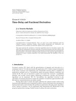
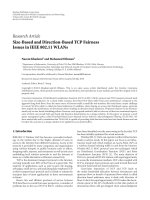
Báo cáo hóa học: " Research Article Multichannel ECG and Noise Modeling: Application to Maternal and Fetal ECG Signals" pdf

Hindawi Publishing Corporation
EURASIP Journal on Advances in Signal Processing
Volume 2007, Article ID 43407, 14 pages
doi:10.1155/2007/43407
Research Article
Multichannel ECG and Noise Modeling: Application to
Maternal and Fetal ECG Signals
Reza Sameni,
1, 2
Gari D. Clifford,
3
Christian Jutten,
2
and Mohammad B. Shamsollahi
1
1
Biomedical Signal and Image Processing Laboratory (BiSIPL), School of Electrical Engineering, Sharif University of Technology,
P.O. Box 11365-9363, Tehran, Iran
2
Laboratoire des Images et des Signaux (LIS), CNRS - UMR 5083, INPG, UJF, 38031 Grenoble Cedex, France
3
Laboratory for Computational Physiology, Harvard-MIT Division of Health Sciences and Technology (HST),
Massachusetts Institute of Technology, Cambridge, MA 02139, USA
Received 1 May 2006; Revised 1 November 2006; Accepted 2 November 2006
Recommended by William Allan Sandham
A three-dimensional dynamic model of the electrical activity of the heart is presented. T he model is based on the single dipole
model of the heart and is later related to the body surface potentials through a linear model which accounts for the temporal
movements and rotations of the cardiac dipole, together with a realistic ECG noise model. The proposed model is also generalized
to maternal and fetal ECG mixtures recorded from the abdomen of pregnant women in single and multiple pregnancies. The
applicability of the model for the evaluation of s ignal processing algorithms is illustrated using independent component analysis.
Considering the difficulties and limitations of recording long-term ECG data, especially from pregnant women, the model de-

scribed in this paper may serve as an effective means of simulation and analysis of a wide range of ECGs, including adults and
fetuses.
Copyright © 2007 Reza Sameni et al. This is an open access article distributed under the Creative Commons Attribution License,
which permits unrestricted use, distribution, and reproduction in any medium, provided the original work is properly cited.
1. INTRODUCTION
The electrical activit y of the cardiac muscle and its relation-
ship with the body surface potentials, namely the electrocar-
diogram (ECG), has been studied with different approaches
ranging from single dipole models to activation maps [1]. The
goal of these models is to represent the cardiac activity in
the simplest and most informative way for specific applica-
tions. However, depending on the application of interest, any
of the proposed models have some level of abstraction, which
makes them a compromise between simplicity, accuracy, and
interpretability for cardiologists. Specifically, it is known that
the single dipole model and its variants [1]areequivalent
source descriptions of the true cardiac potentials. This means
that they can only be used as far-field approximations of the
cardiac activity, and do not have ev ident interpretations in
terms of the underlying electrophysiology [2]. However, de-
spite these intrinsic limitations, the single dipole model still
remains a popular model, since it accounts for 80% to 90%
of the power of the body surface potentials [2, 3].
Statistical decomposition techniques such as principal
component analysis (PCA) [4–7], and more recently indepen-
dent compone nt analysis (ICA) [6, 8–10] have been widely
used as promising methods of multichannel ECG analysis,
and noninvasive fetal ECG extraction. However, there are
many issues such as the interpretation, stability, robustness,
and noise sensitivity of the extracted components. These is-

sues are left as open problems and require further studies by
using realistic models of these signals [11].Notethatmostof
these algorithms have been applied blindly, meaning that the
aprioriinformation about the underlying signal sources and
the propagation media have not been considered. This sug-
gests that by using additional information such as the tempo-
ral dynamics of the cardiac signal (even through approximate
models such as the single dipole model), we can improve the
performance of existing signal processing methods. Exam-
ples of such improvements have been previously reported in
other contexts (see [12, Chapters 11 and 12]).
In recent years, research has been conducted towards the
generation of synthetic ECG signals to facilitate the testing
of signal processing algorithms. Specifical ly, in [13, 14]a
dynamic model has been developed, which reproduces the
morphology of the PQRST complex and its relationship to
the beat-to-beat (RR interval) timing in a single nonlinear
2 EURASIP Journal on Advances in Signal Processing
dynamic model. Considering the simplicity and flexibility
of this model, it is reasonable to assume that it can be eas-
ily adapted to a broad class of normal and abnormal ECGs.
However, previous works are restricted to single-channel
ECG modeling, meaning that the parameters of the model
should be recalculated for each of the recording channels.
Moreover, for the maternal and fetal mixtures recorded from
the abdomen of pregnant women, there are very few works
which have considered both the cardiac source and the prop-
agation media [4, 15, 16].
Real ECG recordings a re always contaminated with noise
and artifacts; hence besides the modeling of the cardiac

sources and the propagation media, it is very important to
have realistic models for the noise sources. Since common
ECG contaminants a re nonstationary and temporally corre-
lated, time-varying dynamic models are required for the gen-
eration of realistic noises.
In the following, a three-dimensional canonical model of
the single dipole vector of the heart is proposed. This model,
which is inspired by the single-channel ECG dynamic model
presented in [13], is later related to the body surface poten-
tials through a linear model that accounts for the temporal
movements and rotations of the cardiac dipole, together with
a model for the generation of realistic ECG noise. The ECG
model is then generalized to fetal ECG signals recorded from
the maternal abdomen. The model described in this paper is
believed to be an effective means of providing realistic simu-
lations of maternal/fetal ECG mixtures in single and multiple
pregnancies.
2. THE CARDIAC DIPOLE VERSUS THE
ELECTROCARDIOGRAM
According to the single dipole model of the heart, the my-
ocardium’s electrical activity may be represented by a time-
varying rotating vector, the origin of which is assumed to be
at the center of the heart as its end sweeps out a quasiperiodic
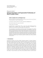
path through the torso. This vector may be mathematically
represented in the Cartesian coordinates, as follows:
d(t)
= x(t)a
x
+ y(t)a
y

+ z(t)a
z
,(1)
where
a
x
, a
y
,anda
z
are the unit vectors of the three body
axes shown in Figure 1. With this definition, and by a ssum-
ing the body volume conductor as a passive resistive medium
which only attenuates the source field [17, 18], any ECG sig-
nal recorded from the body surface would be a linear projec-
tion of the dipole vector d(t) onto the direction of the record-
ing electrode axes v
= aa
x
+ ba
y
+ ca
z
ECG(t) =

d(t), v

=
a · x(t)+b · y(t)+c · z(t). (2)
As a simplified example, consider the dipole source of

d(t) inside a homogeneous infinite-volume conductor. The
potential generated by this dipole at a distance of
|r| is
φ(t)
− φ
0
=
d(t) · r
4πσ|r|
3
=
1
4πσ

x( t)
r
x
|r|
3
+ y(t)
r
y
|r|
3
+ z(t)
r
z
|r|
3


,
(3)
x
y
z
a
x
a
y
a
z
Figure 1: The three body axes, adapted from [3].
where φ
0
is the reference potential, r = r
x
a
x
+r
y
a
y
+r
z
a
z
is the
vector which connects the center of the dipole to the observa-
tion point, and σ is the conductivity of the volume conductor
[3, 17]. Now consider the fact that the ECG signals recorded

from the body surface are the potential differences between
two different points. Equation (3) therefore indicates how the
coefficients a, b,andc in (2) can be related to the radial dis-
tance of the electrodes and the volume conductor material.
Of course, in reality the volume conductor is neither homo-
geneous nor infinite, leading to a much more complex re-
lationship between the dipole source and the body surface
potentials. However even with a complete volume conductor
model, the body surface potentials are linear instantaneous
mixtures of the cardiac potentials [17].
A 3D vector representation of the ECG, namely the vec-
torcardiogram (VCG), is also possible by using three of such
ECG signals. Basically, any set of three linearly indepen-
dent ECG elect rode leads can be used to construct the VCG.
However, in order to achieve an orthonormal representa-
tion that best resembles the dipole vector d(t), a set of
three orthogonal leads that corresponds with the three body
axes is selected. The normality of the representation is fur-
ther achieved by attenuating the different leads with apriori
knowledge of the body volume conductor, to compensate for
the nonhomogeneity of the body thorax [3]. The Frank lead
system [19], and the corrected Frank lead system [20]which
has better orthogonality and normalization, are conventional
methods for recording the VCG.
Based on the single dipole model of the heart, Dower et
al. have developed a transformation for finding the standard
12-lead ECGs from the Frank electrodes [21]. The Dower
transform is simply a 12
× 3 linear transformation between
the standard 12-lead ECGs and the Frank leads, which can

be found from the minimum mean-square error (MMSE)
estimate of a transformation matrix between the two elec-
trode sets. Apparently, the transformation is influenced by
the standard locations of the recording leads and the atten-
uations of the body volume conductor, with respect to each
electrode [22]. The Dower transform and its inverse [23]are
evident results of the single dipole m odel of the heart with
a linear propagation model of the body volume conductor.
Reza Sameni et al. 3
However, since the single dipole model of the heart is not
a perfect representation of the cardiac activity, cardiologists
usually use more than three ECG electrodes (between six to
twelve) to study the cardiac activity [3].
3. HEART DIPOLE VECTOR AND ECG MODELING
From the single dipole model of the heart, it is now e vident
that the different ECG leads can be assumed to be projections
of the heart’s dipole vector onto the recording electrode axes.
All leads are therefore time-synchronized with each other
and have a quasiperiodic shape. Based on the single-channel
ECG model proposed in [13] (and later updated in [24–26]),
the following dynamic model is suggested for the d(t) dipole
vector:
˙
θ
= ω,
˙
x
=−

i

α
x
i
ω
(b
x
i
)
2
Δθ
x
i
exp

−

Δθ
x
i

2
2

b
x
i

2

,

˙
y
=−

i
α
y
i
ω

b
y
i

2
Δθ
y
i
exp

−

Δθ
y
i

2
2

b

y
i

2

,
˙
z
=−

i
α
z
i
ω

b
z
i

2
Δθ
z
i
exp

−

Δθ
z

i

2
2

b
z
i

2

,
(4)
where Δθ
x
i
= (θ − θ
x
i
)mod(2π), Δθ
y
i
= (θ − θ
y
i
)mod(2π),
Δθ
z
i
= (θ − θ

z
i
)mod(2π), and ω = 2πf,where f is the beat-
to-beat heart rate. Accordingly, the first equation in (4)gen-
erates a circular trajectory rotating with the frequency of the
heart rate. Each of the three coordinates of the dipole vec-
tor d(t) is modeled by a summation of Gaussian functions
with the amplitudes of α
x
i
, α
y
i
,andα
z
i
; widths of b
x
i
, b
y
i
,and
b
z
i
; and is located at the rotational angles of θ
x
i
, θ

y
i
,andθ
z
i
.
The intuition behind this set of equations is that the baseline
of each of the dipole coordinates is pushed up and down, as
the trajectory approaches the centers of the Gaussian func-
tions, generating a moving and variable-length vector in the
(x, y, z) space. Moreover, by adding some deviations to the
parameters of (4) (i.e., considering them as r andom variables
rather than deterministic constants), it is possible to generate
more realistic cardiac dipoles with interbeat variations.
This model of the rotating dipole vector is rather general,
since due to the universal approximation property of Gaus-
sian mixtures, any continuous function (as the dipole vector
isassumedtobeso)canbemodeledwithasufficient number
of Gaussian functions up to an arbitrarily close approxima-
tion [27].
Equation (4) can also be thought as a model for the or-
thogonal lead VCG coordinates, with an appropriate scaling
factor for the attenuations of the volume conductor. This
analogy between the orthogonal VCG and the dipole vector
can be used to estimate the parameters of (4) from the three
Frank lead VCG recordings. As an illustration, typical signals
recorded from the Frank leads and the dipole vector mod-
eled by (4) are plotted in Figures 2 and 3.Theparametersof
(4) used for the generation of these figures are presented in
Table 1. These parameters have been estimated from the best

MMSE fitting between N Gaussian functions and the Frank
lead signals. As it can be seen in Table 1, the number of the
Gaussian functions is not necessarily the same for the differ-
ent channels, and can be selected according to the shape of
the desired channel.
3.1. Multichannel ECG modeling
The dynamic model in (4) is a representation of the dipole
vector of the heart (or equivalently the orthogonal VCG
recordings). In order to relate this model to realistic mul-
tichannel ECG signals recorded from the body surface, we
need an additional model to project the dipole vector onto
the body surface by considering the propagation of the
signals in the body volume conductor, the possible rotations
and scalings of the dipole, and the ECG measurement noises.
Following the discussions of Section 2, a rather simplified
linear model which accounts for these measures and is in ac-
cordance with (2)and(3) is suggested as follows:
ECG(t)
= H · R · Λ · s(t)+W(t), (5)
where ECG(t)
N×1
is a vector of the ECG channels recorded
from N leads, s(t)
3×1
= [x(t), y(t), z(t)]
T
contains the three
components of the dipole vector d(t), H
N×3
corresponds to

the body volume conductor model (as for the Dower trans-
formation matrix), Λ
3×3
= diag(λ
x
, λ
y
, λ
z
) is a diagonal ma-
trix corresponding to the scaling of the dipole in each of the
x, y,andz directions, R
3×3
is the rotation matrix for the
dipole vector, and W(t)
N×1
is the noise in each of the N ECG
channels at the time instance of t. Note that H, R,andΛ ma-
trices are generally functions of time.
Although the product of H
· R · Λ may be assumed to
be a single matrix, the representation in (5) has the benefit
that the rather stationary features of the body volume con-
ductor that depend on the location of the ECG electrodes
and the conductivity of the body tissues can be considered in
H, while the temporal interbeat movements of the heart can
be considered in Λ and R, meaning that their average val-
ues are identity matrices in a long-term study: E
t
{R}=I,

E
t
{Λ}=I. In the appendix by using the Givens rotation, a
means of coupling these matrices with external sources such
as the respiration and achieving nonstationary mixtures of
the dipole source is presented.
3.2. Modeling maternal abdominal recordings
By utilizing a dynamic model like (4) for the dipole vector of
the heart, the signals recorded from the abdomen of a preg-
nant woman, containing the fetal and maternal heart com-
ponents can be modeled as follows:
X(t)
=H
m
· R
m
· Λ
m
· s
m
(t)+H
f
· R
f
· Λ
f
· s
f
(t)+W( t),
(6)

where the matrices H
m
, H
f
, R
m
, R
f
, Λ
m
, and, Λ
f
have sim-
ilar definitions as the ones in (5), with the subscripts m and
f referring to the mother and the fetus, respectively. More-
over , R
f
has the additional interpretation that its mean value
4 EURASIP Journal on Advances in Signal Processing
20 2
0.2
0
0.2
0.4
0.6
0.8
1
1.2
1.4
1.6

θ (rads.)
mV
x
Original ECG
Synthetic ECG
(a)
20 2
0.3
0.2
0.1
0
0.1
0.2
0.3
0.4
0.5
θ (rads)
mV
y
Original ECG
Synthetic ECG
(b)
20 2
0.8
0.6
0.4
0.2
0
0.2
0.4

0.6
θ (rads)
mV
z
Original ECG
Synthetic ECG
(c)
Figure 2: Synthetic ECG signals of the Frank lead electrodes.
Table 1: Parameters of the synthetic model presented in (4) for the ECGs and VCG plotted in Figures 2 and 3.
Index(i)1234567891011
α
x
i
(mV) 0.03 0.08 −0.13 0.85 1.11 0.75 0.06 0.10 0.17 0.39 0.03
b
x
i
(rads) 0.09 0.11 0.05 0.04 0.03 0.03 0.04 0.60 0.30 0.18 0.50
θ
i
(rads) −1.09 −0.83 −0.19 −0.07 0.00 0.06 0.22 1.20 1.42 1.68 2.90
α
y
i
(mV) 0.04 0.02 −0.02 0.32 0.51 −0.32 0.04 0.08 0.01 — —
b
y
i
(rads) 0.07 0.07 0.04 0.06 0.04 0.06 0.45 0.30 0.50 — —
θ

j
(rads) −1.10 −0.90 −0.76 −0.11 −0.01 0.07 0.80 1.58 2.90 — —
α
z
i
(mV) −0.03 −0.14 −0.04 0.05 −0.40 0.46 −0.12 −0.20 −0.35 −0.04 —
b
z
i
(rads) 0.03 0.12 0.04 0.40 0.05 0.05 0.80 0.40 0.20 0.40 —
θ
k
(rads) −1.10 −0.93 −0.70 −0.40 −0.15 0.10 1.05 1.25 1.55 2.80 —
(E
t
{R
f
}=R
0
) is not an identity matrix and can be assumed
as the relative position of the fetus with respect to the axes of
the maternal body. This is an interesting feature for modeling
the fetus in the different typical positions such as ve rtex (fe-
tal head-down) or breech (fetal head-up) positions [28]. As
illustrated in Figure 4, s
f
(t) = [x
f
(t), y
f

(t), z
f
(t)]
T
can be
assumed as a canonical representation of the fetal dipole vec-
tor which is defined with respect to the fetal body axes, and
in order to calculate this vector with respect to the maternal
body axes, s
f
(t) should be rotated by the 3D rotation matrix
of R
0
:
R
0
=
⎡
⎢
⎢
⎣
10 0
0cosθ
x
sin θ
x
0 − sin θ
x
cos θ
x

⎤
⎥
⎥
⎦
⎡
⎢
⎢
⎣
cos θ
y
0sinθ
y
010
− sin θ
y
0cosθ
y
⎤
⎥
⎥
⎦
×
⎡
⎢
⎢
⎣
cos θ
z
sin θ
z

0
− sin θ
z
cos θ
z
0
001
⎤
⎥
⎥
⎦
,
(7)
where θ
x
, θ
y
,andθ
z
are the angles of the fetal body planes
with respect to the maternal body planes.
Themodelpresentedin(6)maybesimplyextendedto
multiple pregnancies (twins, triplets, quadruplets, etc.) by
considering additional dynamic models for the other fetuses.
3.3. Fitting the model parameter to real recordings
As previously stated, due to the analogy between the dipole
vector and the orthogonal lead VCG recordings, the number
and shape of the Gaussian functions used in (4)canbeesti-
mated from typical VCG recordings. This estimation requires
a set of orthogonal leads, such as the Frank leads, in order

to calibrate the parameters. There are different possible ap-
proaches for the estimation of the Gaussian function param-
eters of each lead. Nonlinear least-square error (NLSE) meth-
ods, as previously suggested in [26, 29], have been proved
as an effective approach. Otherwise, one can use the A
∗
op-
timization approach adopted in [27], or benefit from the
Reza Sameni et al. 5
0.3
0.2
0.1
0
0.1
0.2
0.3
0.4
1
0.5
0
0.5
0.5
0
0.5
1
1.5
X (mV)
Z (mV)
Y (mV)
T-loop

P-loop
QRS-loop
Figure 3: Typical synthetic VCG loop. Arrows indicate the direc-
tion of rotation. Each clinical lead is produced by mapping this tra-
jectory onto a 1D vector in this 3D space.
X
m
Y
m
Z
m
Maternal VCG
x
f
y
f
z
f
Fetal V CG
Figure 4: Illustration of the fetal and maternal VCGs versus their
body coordinates.
algorithms developed for radial basis functions (RBFs) in the
neural network context [30]. For the results of this paper, the
NLSE approach has been used.
It should be noted that (4) is some kind of canonical rep-
resentation of the heart’s dipole vector; meaning that the am-
plitudes of the Gaussian terms in (4) are not the same as the
ones recorded from the body surface. In fact, using (4)and
(5) to generate synthetic ECG signals, there is an intrinsic in-
determinacy between the scales of the entries of s(t) and the

mixing matrix H, since there is no way to record the t rue
dipole vectors noninvasively. To solve this ambiguity, and
without the loss of generality, it is suggested that we simply
assume the dipole vector to have specific amplitudes, based
on aprioriknowledge of the VCG shape in each of its three
coordinates, using realistic body torso models [31].
As mentioned before, the H mixing matrix in (5)de-
pends on the location of the recording electrodes. So in order
to estimate this matrix, we first calculate the optimal param-
eters of (4) from the Frank leads of a given database. Next the
H matrix is estimated by using an MMSE estimate b etween
the synthetic dipole vector and the recorded ECG channels
of the database. In fact by using the previously mentioned
assumption that E
t
{R}=I and E
t
{Λ}=I, the MMSE
solution of the problem is

H = E

ECG(t) · s(t)
T

E

s(t) · s(t)
T


−1
. (8)
For the case of abdominal recordings, the estimation of
the H
m
and H
f
matrices in (6)ismoredifficult and requires
aprioriinformation about the location of the elec trodes and
a model for the propagation of the maternal and fetal signals
within the maternal thorax and abdomen [16]. However, a
coarse estimation of H
m
can be achieved for a given configu-
ration of abdominal electrodes by using (8) between the ab-
dominal ECG recordings and three orthogonal leads placed
close to the mother’s heart for recording her VCG. Yet the ac-
curate estimation of H
f
requires more information about the
maternal body, and more accurate nonhomogeneous models
of the volume conductor [4].
The ω term introduced in (4) is in general a time-variant
parameter which depends on physiological factors such as
the speed of electrical wave propagation in the cardiac muscle
or the heart rate var iability (HRV) [13]. Furthermore, since
the phase of the respiratory cycle can be derived from the
ECG (or through other means such as amplifying the differ-
ential change in impedance in the thorax; impedance pneu-
mography) and Λ is likely to vary with respiration, it is logi-

cal that an estimation of Λ overtimecanbemadefromsuch
measurements.
The relative average (static) orientation of the fetal heart
with respect to the maternal cardiac source is represented by
R
0
which could be initially determined through a sonogram,
and later inferred by referencing the signal to a large database
of similar-term fetuses. Of course, both Λ and R
0
are func-
tions of the respiration and heart rates, and therefore track-
ing procedures such as expectation maximization (EM) [32],
or Kalman filter (KF) may be required for online adaptation
of these parameters [25, 33].
4. ECG NOISE MODELING
An important issue that should be considered in the mod-
eling of realistic ECG signals is to model realistic noise
sources. Following [34], the most common high-amplitude
ECG noises that cannot be removed by simple inband filter-
ing are
(i) baseline wander (BW);
(ii) muscle artifact (MA);
(iii) electrode movement (EM).
For the fetal ECG signals recorded from the maternal ab-
domen, the following may also be added to this list:
(i) maternal ECG;
(ii) fetal movements;
(iii) maternal uterus contractions;
(iv) changes in the conductivity of the maternal volume

conductor due to the development of the vernix caseosa
layer around the fetus [4].
These noises are typically very nonstationary in time and
colored in spectrum (having long-term correlations). This
6 EURASIP Journal on Advances in Signal Processing
means that white noise or stationary colored noise is gener-
ally insufficient to model ECG noise. In practice, researchers
have preferred to use real ECG noises such as those found
in the MIT-BIH non-stress test database (NSTDB) [35, 36],
with varying signal-to-noise ratios (SNRs). However, as ex-
plained in the following, parametric models such as time-
varying autoregressive (AR) models can be used to generate
realistic ECG noises which follow the nonstationarity and the
spectral shape of real noise. The parameters of this model can
be trained by using real noises such as the NSTDB. Having
trained the model, it can be driven by white noise to gener-
ate different instances of such noises, with almost identical
temporal and spectr a l characteristics.
There are different approaches for the estimation of time-
varying AR parameters. An efficientapproachthatwasem-
ployed in this work is to reformulate the AR model estima-
tion problem in the form of a standard KF [37]. In a recent
work, a similar approach has been effectively used for the
time-varying analysis of the HRV [38].
For the time series of y
n
, a time-varying AR model of or-
der p can be described as follows:
y
n

=−a
n1
y
n−1
− a
n2
y
n−2
−···−a
np
y
n−p
+ v
n
=−

y
n−1
, y
n−2
, , y
n−p

⎡
⎢
⎢
⎢
⎢
⎢
⎣

a
n1
a
n2
.
.
.
a
np
⎤
⎥
⎥
⎥
⎥
⎥
⎦
+ v
n
,
(9)
where v
n
is the input white noise and the a
ni
(i = 1, , p)
coefficients are the p time varying AR parameters at the time
instance of n. So by defining x
n
= [a
n1

, a
n2
, , a
np
]
T
as a
state vector, and h
n
=−[y
n−1
, y
n−2
, , y
n−p
]
T
,wecanre-
formulate the problem of AR parameter estimation in the KF
form as follows:
x
n+1
= x
n
+ w
n
,
y
n
= h

T
n
x
n
+ v
n
,
(10)
where we have assumed that the temporal evolution of the
time-varying AR parameters follows a random walk model
with a white Gaussian input noise vector w
n
. This approach
is a conventional and practical assumption in the KF context
when there is no aprioriinformation about the dynamics of
a state vector [37].
To solve the standard KF equations [37], we also require
the expected initial state vector
x
0
= E{x
0
},itscovariance
matrix P
0
= E{x
0
x
T
0

}, the covariance matrices of the process
noise Q
n
= E{w
n
w
T
n
}, and the measurement noise variance
r
n
= E{v
n
v
T
n
}.
x
0
can be estimated from a global (time-invariant) AR
model fitting over the whole samples of y
n
, and its covari-
ance matrix (P
0
) can be selected large enough to indicate the
imprecision of the initial estimate. The effects of these ini-
tial states are of less importance and usually vanish in time,
under some general convergence properties of KFs.
By considering the AR parameters to be uncorrelated, the

covariance matrix of Q
n
can be selected as a diagonal matrix.
0 102030405060
0
0.5
1
1.5
2
2.5
3
Time (s)
mV
(a)
0 102030405060
0
0.5
1
1.5
2
2.5
3
Time (s)
mV
(b)
Figure 5: Typical segment of ECG BW noise (a) original and (b)
synthetic.
The selection of the ent ries of this matrix depends on the ex-
tent of y
n

’s nonstationarity. For quasistationary noises, the
diagonal entries of Q
n
are rather small, while for highly non-
stationary noises, the y are large. Generally, the selection of
this matrix is a compromise between convergence rate and
stability. Finally, r
n
is selected according to the desired vari-
ance of the output noise.
To complete the discussion, the AR model order should
also be selected. It is known that for stationary AR models,
there are information-based criteria such as the Akaike infor-
mation criterion (AIC) for the selection of the optimal model
order. However, for time-varying models, the selection is not
as straightforward since the model is dynamically evolving in
time. In general, the model order should be less than the op-
timal order of a global time-invariant model. For example,
in this study, an AR order of twelve to sixteen was found to
be sufficient for a time-invariant AR model of BW noise, us-
ing the AIC. Based on this, the order of the time-variant AR
model was selected to be twelve, which led to the generation
of realistic noise samples.
Now having the time-varying AR model, it is possible to
generate noises with different variances. As an illustration,
in Figure 5, a one-minute long segment of BW with a sam-
pling rate of 360 Hz, taken from the NSTDB [35, 39], and
the synthetic BW noise generated by the proposed method
are depicted. The frequency response magnitude of the time-
varying AR filter designed for this BW noise is depicted in

Figure 6. As it can be seen, the time-var ying AR model is act-
ing as an adaptive filter which is adapting its frequency re-
sponse to the contents of the nonstationary noise.
It should be noted that since the vector h
n
varies with
time, it is very important to monitor the covariance matrix
of the KF’s error and the innovation signal, to be sure about
the stability and fidelity of the filter.
Reza Sameni et al. 7
0 20 40 60 80 100 120 140 160 180
80
60
40
20
0
20
Frequency (Hz)
Frequency response
magnitude (dB)
Figure 6: Frequency response magnitudes of 32 segments of the
time-var ying AR filters for the baseline wander noises of the
NSTDB. This figure illustrates how the AR filter responses are evolv-
ing in time.
By using the KF framework, it is also possible to monitor
the stationarity of the y
n
signals, and to update the AR pa-
rameters as they tend to become nonstationary. For this, the
variance of the innovation signal should be monitored, and

the KF state vectors (or the AR parameters) should be up-
dated only whenever the variance of the innovation increases
beyond a predefined value. There have also been some ad hoc
methods developed for updating the covariance matrices of
the observation and process noises and to prevent the diver-
gence of the KF [38].
For the studies in which a continuous measure of the
noise color effect is required, the spectral shape of the out-
put noise can also be altered by manipulating the poles of the
time-varying AR model over the unit circle, which is iden-
tical to warping the frequency axis of the AR filter response
[40].
5. RESULTS
The approach presented in this work for generating synthetic
ECG sig nals is believed to have interesting applications from
both the theoretical and practical points of view. Here we will
study the accuracy of the synthetic model and a special case
study.
5.1. The model accuracy
In this example, the model accuracy will be studied for a typi-
cal ECG signal of the Physikalisch-Technische Bundesanstalt
Diagnostic ECG Database (PTBDB) [41–43]. The database
consists of the standard twelve-channel ECG recordings
and the three Frank lead VCGs. In order to have a clean
template for extracting the model parameters, the signals
are pre-processed by a bandpass filter to remove the baseline
wander and high-frequency noises. The ensemble average of
the ECG is then extracted from each channel. Next, the pa-
rameters of the Gaussian functions of the synthetic model are
extracted from the ensemble average of the Frank lead VCGs

by using the nonlinear least-squares procedure explained in
Section 3.3. T he Original VCGs and the synthetic ones gen-
erated by using five and nine Gaussian functions are depicted
in Figures 7(a)–7(c) for comparison. The mean-square error
Table 2: The percentage of MSE in the synthetic VCG channels us-
ing five and nine Gaussian functions.
VCG channel 5 Gaussians 9 Gaussians
V
x
1.24 0.09
V
y
1.68 0.15
V
z
3.60 0.12
Table 3: The percentage of MSE in the ECGs reconstructed by
Dower transformation from the original VCG and from the syn-
thetic VCG using five and nine Gaussian functions.
ECG channel Original VCG 5 Gaussians 9 Gaussians
V
1
0.78 2.06 0.86
V
2
0.67 3.14 0.72
V
6
0.16 1.12 0.19
(MSE) of the two synthetic VCGs with respect to the true

VCGs are listed in Ta ble 2.
The H matrix defined in (5) may also be calculated
by solving the MMSE transformation between the ECG
and the three VCG channels (similar to (8)). As with the
Dower transform, H can be used to find approximative ECGs
from the three original VCGs or the synthetic VCGs. In
Figures 7(d)–7(f), the original ECGs of channels V
1
, V
2
,and
V
6
, and the approximative ones calculated from the VCG are
compared with the ECGs calculated from the synthetic VCG
using five and nine Gaussian functions for one ECG cycle.
As it can be seen in these results, the ECGs which are re-
constructed from the synthetic VCG model have significantly
improved as the number of Gaussian functions has been in-
creased from five to nine, and the resultant signals very well
resemble the ECGs which have been reconstructed from the
original VCG by using the Dower transform. The model im-
provement is especially notable, around the asymmetric seg-
ments of the ECG such as the T-wave.
However, it should be noted that the ECG signals which
are reconstructed by using the Dower transform (either
from the original VCG or the synthetic ones) do not per-
fectly match the true recorded ECGs, especially in the low-
amplitude segments such as the P-wave. This in fact shows
the intrinsic limitation of the single dipole model in repre-

senting the low-amplitude components of the ECG which
require more than three dimensions for their accurate rep-
resentation [11]. The MSE of the calculated ECGs of Figures
7(d)–7(f) with respect to the true ECGs is listed in Ta ble 3.
5.2. Fetal ECG extraction
We will now present an application of the proposed model
for evaluating the results of source separation algorithms.
To generate synthetic maternal abdominal recordings,
consider two dipole vectors for the mother and the fetus as
defined in (4). The dipole vector of the mother is assumed
to have the parameters listed in Ta ble 1 with a heart rate of
f
m
= 0.9 Hz, and the fetal dipole is assumed to have the pa-
rameters listed in Table 4,withaheartbeatof f
f
= 2.2 Hz.
8 EURASIP Journal on Advances in Signal Processing
00.25 0.50.75 1
0.8
0.4
0.2
0
0.4
0.8
1.2
1.6
Time (s)
mV
Original VCG

Synthetic VCG (5 kernels)
Synthetic VCG (9 kernels)
(a) V
x
00.25 0.50.75 1
0.8
0.6
0.4
0.2
0
0.2
0.4
0.6
Time (s)
mV
Original VCG
Synthetic VCG (5 kernels)
Synthetic VCG (9 kernels)
(b) V
y
00.25 0.50.75 1
1
0.8
0.6
0.4
0.2
0
0.2
0.4
0.6

Time (s)
mV
Original VCG
Synthetic VCG (5 kernels)
Synthetic VCG (9 kernels)
(c) V
z
00.25 0.50.75 1
2.5
2
1.5
1
0.5
0
0.5
1
Time (s)
mV
Real ECG
Dower reconstructed ECG
Synthetic ECG using 5 kernels
Synthetic ECG using 9 kernels
(d) V
1
00.25 0.50.75 1
3
2.5
2
1.5
1

0.5
0
0.5
1
1.5
Time (s)
mV
Real ECG
Dower reconstructed ECG
Synthetic ECG using 5 kernels
Synthetic ECG using 9 kernels
(e) V
2
00.25 0.50.75 1
1
0.5
0
0.5
1
1.5
2
Time (s)
mV
Real ECG
Dower reconstructed ECG
Synthetic ECG using 5 kernels
Synthetic ECG using 9 kernels
(f) V
6
Figure 7: Original versus synthetic VCGs and ECGs using 5 and 9 Gaussian functions. For comparison, the ECG reconstructed from the

Dower transformation is also depicted in (d)–(f) over the original ECGs. The synthetic VCGs and ECGs have been vertically shifted 0.2mV
forbettercomparison,refertotextfordetails.
As seen in Table 4, the amplitudes of the Gaussian terms used
for modeling the fetal dipole have been chosen to be an order
of magnitude smaller than their maternal counterparts.
Further consider the fetus to be in the normal vertex po-
sition shown in Figure 8, with its head down and its face
towards the right arm of the mother. To simulate this po-
sition, the angles of R
0
defined in (7) can be selected as
follows: θ
x
=−3π/4 to rotate the fetus around the x-axis
of the maternal body to place it in the head-down position,
θ
y
= 0 to indicate no fetal rotation around the y-axis, and
θ
z
=−π/2 to rotate the fetus towards the right arm of the
mother.
1
Now according to (6), to model maternal abdominal sig-
nals, the transformation matrices of H
m
and H
f
are required,
1

The negative signs of θ
x
, θ
y
,andθ
z
are due to the fact that, by definition,
R
0
is the matrix which transforms the fetal coordinates to the maternal
coordinates.
Reza Sameni et al. 9
Table 4: Parameters of the synthetic fetal dipole used in Section 5.2.
Index (i)1 2 3 4 5
α
x
i
(mV) 0.007 −0.011 0.13 0.007 0.028
b
x
i
(rads) 0.10.03 0.05 0.02 0.3
θ
i
(rads) −0.7 −0.17 0 0.18 1.4
α
y
i
(mV) 0.004 0.03 0.045 −0.035 0.005
b

y
i
(rads) 0.10.05 0.03 0.04 0.3
θ
j
(rads) −0.9 −0.08 0 0.05 1.3
α
z
i
(mV) −0.014 0.003 −0.04 0.046 −0.01
b
z
i
(rads) 0.10.40.03 0.03 0.3
θ
k
(rads) −0.8 −0.3 −0.10.06 1.35
8
6+, 8+
7
7+
1
3
2
5
4
Navel
Front view
Z
m

Y
m
X
m
(a)
Left Right
Fetal heart
Maternal heart
6
6+, 7 ,8+,8
7+
3, 4
5
1, 2
Navel
Top v i ew
Z
m
Y
m
X
m
(b)
Figure 8: Model of the maternal torso, with the locations of the
maternal and fetal hearts and the simulated electrode configuration.
which depend on the maternal and fetal body volume con-
ductors as the propagation medium. As a simplified case,
consider this volume conductor to be a homogeneous in-
finite medium which only contains the two dipole sources
of the mother and the fetus. Also consider five abdominal

electrodes with a reference electrode of the maternal navel,
and three thoracic electrode pairs for recording the maternal
ECGs, as illustrated in Figure 8. T his electrode configuration
is in accordance with real measurement systems presented in
[9, 44, 45], in which several electrodes are placed over the
maternal abdomen and thorax to record the fECG in any fetal
position without changing the electrode configuration. From
the source separa tion point of view, the maximal spatial di-
versity of the electrodes with respect to the signal sources
such as the maternal and fetal hearts is expected to improve
the separation performance. The location of the maternal
and fetal hearts and the recording electrodes are presented in
Table 5 for a typical shape of a pregnant woman’s abdomen.
In this table, the maternal navel is considered as the origin of
the coordinate system.
Previous studies have shown that low conductivity layers
which are formed around the fetus (like the vernix caseosa)
have great influence on the attenuation of the fetal sig-
nals. The conductivity of these layers has been measured to
be about 10
6
times smaller than their surrounding tissues;
meaning that even a very thin layer of these tissues has con-
siderable effect on the fetal components [4]. The complete
solution of this problem which encounters the conductivities
of different layers of the body tissues requires a much more
sophisticated model of the volume conductor, w h ich is be-
yond the scope of this example. For simplicity, we define the
constant terms in (3)asκ
.

= 1/4πσ,andassumeκ = 1 for the
maternal dipole and κ
= 0.1 for the fetal dipole. These values
of κ lead to simulated signals having maternal to fetal peak-
amplitude ratios, that are in accordance w ith real abdominal
measurements such as the DaISy database [44].
Using (2)and(3), the electrode locations, and the vol-
ume conductor conductivities, we can now calculate the co-
efficients of the transformation between the dipole vector
and each of the recording electrodes for both the mother and
the fetus (Table 6).
The next step is to generate realistic ECG noise. For this
example, a one-minute mixture of noises has been produced
by summing normalized portions of real baseline wan-
der, muscle artifacts, and elec trode movement noises of the
NSTDB [35, 39]. The time-varying AR coefficient described
in Section 4 may be calculated for this mixture. We can now
generate different instances of synthetic ECG noise by using
different instances of white noise as the input of the time-
varying AR model. Normalized portions of these noises can
be added to the synthetic ECG to achieve synthetic ECGs
with desired SNRs.
A five-second segment of eight maternal channels gener-
ated with this method can be seen in Figure 9. In this exam-
ple, the SNR of each channel is 10 dB. Also as an illustration,
the 3D VCG loop constru cted from a combination of three
pairs of the electrodes is depicted in Figure 10.
As previously mentioned, the multichannel synthetic
recordings described in this paper can be used to study the
performance of the signal processing tools previously devel-

oped for ECG analysis. As a typical example, the JADE ICA
algorithm [46] was applied to the eight synthetic channels to
extract eight independent components. The resultant inde-
pendent components (ICs) can be seen in Figure 11.
According to these results, three of the extracted ICs cor-
respond to the maternal ECG, and two with the fetal ECG.
The other channels are mainly the noise components, but
still contain some elements of the fetal R-peaks. Moreover
10 EURASIP Journal on Advances in Signal Processing
Table 5: The simulated electrode and heart locations.
∗
Index
Abdominal leads Thoracic lead pairs Heart locations
123456+ 6− 7+ 7− 8+ 8− Maternal heart Fetal heart
x (cm) −5 −5 −5 −5 −5 −10 −35 −10 −10 −10 −10 −25 −15
y (cm)
−7 −77 7−1 10 10 0 10 10 10 7 −4
z (cm)
7 −77−7 −5 18 18 15 15 18 24 20 2
∗
The maternal navel is assumed as the center of the coordinate system and the reference electrode for the abdominal leads.
Table 6: The calculated mixing matrices for the maternal and fetal
dipole vectors.
H
T
m
=10
−3
×
⎡

⎢
⎢
⎣
0.23 −0.30 0.76 −0.18 −0.15 12.41 −0.70 −0.20
−0.46 −0.09 0.20 0.20 −0.02 −1.68 −2.07 −0.04
−0.05 0.01 −0.39 −0.14 −0.13 1.12 0.23 −2.21
⎤
⎥
⎥
⎦
H
T
f
=10
−3
×
⎡
⎢
⎢
⎣
0.25 −0.01 −0.13 −0.20 0.11 0.13 0.10 0.04
−0.30 −0.22 0.18 0.11 0.05 0.08 −0.05 0.11
0.37
−0.29 0.18 −0.12 −0.30 0.09 0.26 0.05
⎤
⎥
⎥
⎦
some peaks of the fetal components are still valid in the ma-
ternal components, meaning that ICA has failed to com-

pletely separate the maternal and fetal components.
To explain these results, we should note that the dipole
model presented in (4) has three linearly independent di-
mensions. This means that if the synthetic signals were noise-
less, we could only have six linearly independent channels
(three due to the maternal dipole and three due to the fetal),
and any additional channel would be a linear combination of
the others. However, for noisy signals, additional dimensions
are introduced which correspond to noise. In the ICA con-
text, it is known that the ICs extracted from noisy recordings
can be very sensitive to noise. In this example in particular,
the coplanar components of the maternal and fetal subspaces
are more sensitive and may be dominated by noise. This ex-
plains why the traces of the fetal component are seen among
the maternal components, instead of being extracted as an
independent component [11]. The quality of the extracted
fetal components may be improved by denoising the signals
with, for example, wavelet denoising techniques, before ap-
plying ICA [10].
This example demonstrates that by using the proposed
model for body surface recordings with different source sepa-
ration algorithms, it is possible to find interesting interpreta-
tions and theoretical bases for prev iously reported empirical
results.
6. DISCUSSIONS AND CONCLUSIONS
In this paper, a three-dimensional model of the dipole vector
of the heart was presented. The model was then used for the
generation of synthetic multichannel signals recorded from
the body surface of normal adults and pregnant women. A
practical means of generating realistic ECG noises, which

are recorded in real conditions, was also developed. The
effectiveness of the model, particularly for fetal ECG stud-
ies, was illustrated through a simulated example. Consid-
ering the simplicity and generality of the proposed model,
there are many other issues which may be addressed in fu-
ture works, some of which will now be described.
In the presented results, an intrinsic limitation of the sin-
gle dipole model of the heart was shown. To overcome this
limitation, more than three dimensions may be used to rep-
resent the cardiac dipole model in (4). In recent works, it has
been shown that up to five or six dimensions may be neces-
sary for the better representation of the cardiac dipole [ 11].
In future works, the idea of extending the single dipole
model to moving dipoles which have higher accuracies can
also be studied [2]. For such an approach, the dynamic repre-
sentation in (4) can be ver y useful. In fact, the moving dipole
would be simply achieved by adding oscillatory terms to the
x, y,andz coordinates in (4) to represent the speed of the
heart’s dipole movement. In this case, besides the model-
ing aspect of the proposed approach, it can also be used as
a model-based method of verifying the performance of dif-
ferent heart models.
Looking back to the synthetic dipole model in (4), it
is seen that this dynamic model could have also been pre-
sented in the direct form (by simply integrating these equa-
tions with respect to time). However the state-space repre-
sentation has the benefit of allowing the study of the evo-
lution of the signal dynamics using state-space approaches
[37]. Moreover, the combination of (4)and(5)canbeeffec-
tively used as the basis for Kalman filtering of noisy ECG ob-

servations, where (4) represents the underlying dynamics of
the noisy recorded channels. In some related works, the au-
thors have developed a nonlinear model-based Bayesian fil-
tering approach (such as the extended Kalman filter) for de-
noising single-channel ECG signals [25, 33, 47], which led to
superior results compared with conventional denoising tech-
niques. However, the extension of such proposed approaches
for multichannel recordings requires the multidimensional
modeling of the heart dipole vector which is presented in
this paper. In fact, multiple ECG recordings can be used as
multiple observations for the Kalman filtering procedure,
which is believed to further improve the denoising results.
The Kalman filtering framework is also believed to be exten-
sible to the filtering and extraction of fetal ECG components.
Reza Sameni et al. 11
012345
0.2
0.1
0
0.1
0.2
0.3
0.4
Time (s)
Ch
1
(mV)
(a) Channel 1
012345
0.6

0.5
0.4
0.3
0.2
0.1
0
Time (s)
Ch
2
(mV)
(b) Channel 2
012345
0
0.5
1
Time (s)
Ch
3
(mV)
(c) Channel 3
012345
0.3
0.2
0.1
0
0.1
Time (s)
Ch
4
(mV)

(d) Channel 4
012345
0.25
0.2
0.15
0.1
0.05
0
0.05
Time (s)
Ch
5
(mV)
(e) Channel 5
012345
5
0
5
10
15
20
Time (s)
Ch
6
(mV)
(f) Channel 6
012345
2
1.5
1

0.5
0
0.5
1
Time (s)
Ch
7
(mV)
(g) Channel 7
012345
1.5
1
0.5
0
0.5
1
1.5
2
Time (s)
Ch
8
(mV)
(h) Channel 8
Figure 9: Synthetic multichannel signals from the maternal abdomen (channels 1–5) and thorax (channels 6–8). Notice the small fetal
components with a frequency almost twice the maternal heart rate in the abdominal channels.
5
0
5
10
15

20
0.5
0
0.5
1
1.5
0.2
0
0.2
0.4
Ch
6
(mV)
Ch
3
-Ch
1
(mV)
Ch
4
-Ch
2
(mV)
Figure 10: Synthetic mixture of the maternal and fetal VCGs, using
a combination of the leads defined in Table 5.
In this case, the dynamic evolutions of the fetal and maternal
dipoles are modeled w ith (4), and (6) can be assumed as the
observation equation.
Following the discussions in Section 3 , it is known that
Gaussian mixtures are capable of modeling any ECG signal,

even with asymmetric shapes such as the T-wave (which is
rather common in real recordings). However in these cases,
two or more Gaussian terms or a log-normal function may
be required to model the asymmetric shape. For such ap-
plications, it could be simpler to substitute the Gaussian
functions with naturally asymmetric functions, such as the
Gumbel function which has a Gaussian shape that is skewed
towards the right- or left-side of its peak [48]. A log-normal
distribution may give the same results as the Gumbel, but the
Gumbel function allows a more intuitive parameterization in
terms of the width, and hence onsets and offsets in the ECG.
This may be useful for determining the end of the T-wave,
for example, with a high degree of accuracy.
APPENDIX
TIME-VARYING VOLUME CONDUCTOR MODELS
As mentioned in Section 3, the H, R,andΛ matrices are
generally functions of time, having oscillations which are
coupled with the respiration rate or the heart beat. This
oscillatory coupling may be modeled by using the idea of
Givens rotation matrices [49].
In terms of geometric rotations, any rotation in the N-
dimensional space can be decomposed into L
= N(N − 1)/2
rotations corresponding to the number of possible rotation
planes in the N-dimensional space. This explains why N-
dimensional rotation matrices, also known as orthonormal
matrices,haveonlyL degrees of freedom. With this expla-
nation, any orthonormal matrix can be decomposed into L
single rotations, as follows:
R

=

i=1, ,N−1, j=i+1, ,N
R
ij
,(A.1)
where R
ij
is the Givens rotation matrix of the i– j plane, de-
rived from an N-dimensional identity matrix with the four
following changes in its entries:
R
ij
(i, i) = cos

θ
ij

, R
ij
(i, j) = sin

θ
ij

,
R
ij
( j, i) =−sin


θ
ij

, R
ij
( j, j) = cos

θ
ij

,
(A.2)
and θ
ij
is the rotation angle between the i and j axes, in the
12 EURASIP Journal on Advances in Signal Processing
012345
8
6
4
2
0
2
Time (s)
IC
1
(a) IC
1
012345
2

1
0
1
2
3
4
5
Time (s)
IC
2
(b) IC
2
012345
4
2
0
2
4
6
8
10
Time (s)
IC
3
(c) IC
3
012345
2
1
0

1
2
3
Time (s)
IC
4
(d) IC
4
012345
5
4
3
2
1
0
1
Time (s)
IC
5
(e) IC
5
012345
3
2
1
0
1
2
Time (s)
IC

6
(f) IC
6
012345
3
2
1
0
1
2
3
Time (s)
IC
7
(g) IC
7
012345
2
0
2
4
Time (s)
IC
8
(h) IC
8
Figure 11: Independent components (ICs) extracted from the synthetic multichannel recordings. Strong maternal presence can be seen in
the first three components. Fetal cardiac activity can be clearly seen in the last three components.
i–j plane. The R
0

matrix presented in (7)isa3Dexampleof
the general rotation in (A.1).
Now in order to achieve a time-varying rotation matrix
which is coupled with an external source, such as the respira-
tion rate or heart beat (either of the adult or the fetus), any of
the θ
ij
rotation ang les can oscillate with the external source
frequency, as follows:
θ
ij
(t) = θ
max
ij
sin(2πft), (A.3)
where θ
max
ij
is the maximum deviation of the θ
ij
rotation
angle, and f is the frequency of the external source. The
axes which are coupled with the oscillatory source depend
on the nature of the sources of interest and the geometry
of the problem (i.e., the relative location and distance of the
sources), and apparently depending on this geometry, other
means of coupling are also possible.
The presented time-varying rotation matrices can be
used to model the rotation matrices of the synthetic ECG
models defined in (5)and(6), or as multiplicative factors for

the H matrices in these equations.
ACKNOWLEDGMENTS
The authors would like to acknowledge the support of
the Iranian-French Scientific Cooperation Program (PAI
Gundishapur), the Iran Telecommunication Research Cen-
ter (ITRC), the US National Institute of Biomedical Imaging
and Bioengineering under Grant no. R01 EB001659.
REFERENCES
[1] O. D
¨
ossel, “Inverse problem of electro- and magnetocardio-
graphy: review and recent progress,” International Journal of
Bioelectromagnetism, vol. 2, no. 2, 2000.
[2] A. van Oosterom, “Beyond the dipole; modeling the genesis of
the electrocardiogram,” in 100 Years Einthove n , pp. 7–15, The
Einthoven Foundation, Leiden, The Netherlands, 2002.
[3] J. A. Malmivuo and R. Plonsey, Eds., Bioelectromagnetism,
Principles and Applications of Bioelectric and Biomagnetic
Fields, Oxford University Press, New York, NY, USA, 1995.
[4] T. Oostendorp, “Modeling the fetal ECG,” Ph.D. dissertation,
K. U. Nijmegen, Nijmegen, The Netherlands, 1989.
[5] P. P. Kanjilal, S. Palit, and G. Saha, “Fetal ECG extraction from
single-channel maternal ECG using singular value decompo-
sition,” IEEE Transactions on Biomedical Engineering, vol. 44,
no. 1, pp. 51–59, 1997.
[6] P. Gao, E C. Chang, and L. Wyse, “Blind separation of fetal
ECG from single mixture using SVD and ICA,” in Proceedings
of the Joint Conference of the 4th International Conference on In-
formation, Communications and Signal Processing, and the 4th
Pacific Rim Conference on Multimedia (ICICS-PCM ’03), vol. 3,

pp. 1418–1422, Singapore, December 2003.
[7] D. Callaerts, W. Sansen, J. Vandewalle, G. Vantrappen, and J.
Janssen, “Description of a real-time system to extract the fe-
tal electrocardiogram,” Clinical Physics and Physiological Mea-
surement, vol. 10, supplement B, pp. 7–10, 1989.
[8] L. De Lathauwer, B. De Moor, and J. Vandewalle, “Fetal elec-
trocardiogram extraction by blind source subspace separa-
tion,” IEEE Transactions on Biomedical Engineering, vol. 47,
no. 5, pp. 567–572, 2000.
[9] F. Vrins, C. Jutten, and M. Verleysen, “Sensor array and elec-
trode selection for non-invasive fetal electrocardiogram ex-
traction by independent component analysis,” in Proceedings
of 5th International Conference on Independent Component
Analysis and Blind Signal Separation (ICA ’04),C.G.Puntonet
and A. Prieto, Eds., vol. 3195 of Lecture Notes in Computer Sci-
ence, pp. 1017–1014, Granada, Spain, September 2004.
[10] B. Azzerboni, F. La Foresta, N. Mammone, and F. C. Morabito,
“A new approach based on wavelet-ICA algorithms for fetal
electrocardiogram extraction,” in Proceedings of 13th European
Reza Sameni et al. 13
Symposium on Artificial Neural Networks (ESANN ’05),pp.
193–198, Bruges, Belgium, April 2005.
[11] R. Sameni, C. Jutten, and M. B. Shamsollahi, “What ICA
provides for ECG processing: application to noninvasive fe-
tal ECG extraction,” in Proceedings of the International Sym-
posium on Signal Processing and Information Technology
(ISSPIT ’06), pp. 656–661, Vancouver, Canada, August 2006.
[12] A. Cichocki and S. Amari, Eds., Adaptive Blind Signal and Im-
age Processing, John Wiley & Sons, New York, NY, USA, 2003.
[13] P.E.McSharry,G.D.Clifford, L. Tarassenko, and L. A. Smith,

“A dynamical model for generating synthetic electrocardio-
gram signals,” IEEE Transactions on Biomedical Engineering,
vol. 50, no. 3, pp. 289–294, 2003.
[14] P. E. McSharry and G. D. Clifford, ECGSYN - a realistic ECG
waveform generator, />ecgsyn/.
[15] P. Bergveld and W. J. H. Meijer, “A new technique for the sup-
pression of the MECG,” IEEE Transactions on Biomedical En-
gineering, vol. 28, no. 4, pp. 348–354, 1981.
[16] W. J. H. Meijer and P. Bergveld, “The simulation of the ab-
dominal MECG,” IEEE Transactions on Biomedical Engineer-
ing, vol. 28, no. 4, pp. 354–357, 1981.
[17] D. B. Geselowitz, “On the theory of the electrocardiogram,”
Proceedings of the IEEE, vol. 77, no. 6, pp. 857–876, 1989.
[18] J. Bronzino, Ed., The Biomedical Engineering Handbook,CRC
Press, Boca Raton, Fla, USA, 2nd edition, 2000.
[19] E. Frank, “An accurate, clinically practical system for spatial
vectorcardiography,” Circulation, vol. 13, no. 5, pp. 737–749,
1956.
[20] G. F. Fletcher, G. Balady, V. F. Froelicher, L. H. Hartley, W. L.
Haskell, and M. L. Pollock, “Exercise standards: a statement
for healthcare professionals from the American Heart Associ-
ation,” Circulation, vol. 91, no. 2, pp. 580–615, 1995.
[21] G.E.Dower,H.B.Machado,andJ.A.Osborne,“Onderiving
the electrocardiogram from vectorcardiographic leads,” Clini-
cal Cardiology, vol. 3, no. 2, pp. 87–95, 1980.
[22] L. Had
ˇ
zievski, B. Bojovi
´
c, V. Vuk

ˇ
cevi
´
c, et al., “A novel mobile
transtelephonic system with synthesized 12-lead ECG,” IEEE
Transactions on Information Technology in Biomedicine, vol. 8,
no. 4, pp. 428–438, 2004.
[23] L. Edenbrandt and O. Pahlm, “Vectorcardiogram synthesized
from a 12-lead ECG: superiority of the inverse Dower matrix,”
Journal of Electrocardiology, vol. 21, no. 4, pp. 361–367, 1988.
[24] G. D. Clifford and P. E. McSharry, “A realistic coupled non-
linear artificial ECG, BP, and respiratory signal generator for
assessing noise performance of biomedical signal processing
algorithms,” in Fluctuations and Noise in Biological, Biophysi-
cal, and Biomedical Systems II, vol. 5467 of Proceedings of SPIE,
pp. 290–301, Maspalomas, Spain, May 2004.
[25] R. Sameni, M. B. Shamsollahi, C. Jutten, and M. Babaie-Zade,
“Filtering noisy ECG signals using the extended Kalman fil-
ter based on a modified dynamic ECG model,” in Proceedings
of the 32nd Annual International Conference on Computers in
Cardiology, pp. 1017–1020, Lyon, France, September 2005.
[26] G. D. Clifford, “A novel framework for signal representation
and source separation: applications to filtering and segmenta-
tion of biosignals,” Journal of Biological Systems, vol. 14, no. 2,
pp. 169–183, 2006.
[27] J. Ben-Arie and K. R. Rao, “Nonorthogonal signal representa-
tion by Gaussians and Gabor functions,” IEEE Transactions on
Circuits and Systems II: Analog and Digital Signal Processing,
vol. 42, no. 6, pp. 402–413, 1995.
[28] Fetal positions, WebMD, />tools/1/slide

fetal pos.htm.
[29] G. D. Clifford, A. Shoeb, P. E. McSharry, and B. A. Janz,
“Model-based filtering, compression and classification of the
ECG,” International Journal of Bioelectromagnetism, vol. 7,
no. 1, pp. 158–161, 2005.
[30] C. Bishop, Neural Networks for Pattern Recognition,Oxford
University Press, New York, NY, USA, 1995.
[31] L. Weixue and X. Ling, “Computer simulation of epicardial
potentials using a heart-torso model with realistic geometry,”
IEEE Transactions on Biomedical Engineering,vol.43,no.2,pp.
211–217, 1996.
[32] L. Frenkel and M. Feder, “Recursive expectation-maxi-
mization (EM) algorithms for time-varying parameters with
applications to multiple target tracking,” IEEE Transactions on
Signal Processing, vol. 47, no. 2, pp. 306–320, 1999.
[33] R. Sameni, M. B. Shamsollahi, C. Jutten, and G. D. Clifford, “A
nonlinear Bayesian filtering framework for ECG denoising,” to
appear in IEEE Transactions on Biomedical Engineering.
[34] G. M. Friesen, T. C. Jannett, M. A. Jadallah, S. L. Yates, S. R.
Quint, and H. T. Nagle, “A comparison of the noise sensitiv-
ity of nine QRS detection algorithms,” IEEE Transactions on
Biomedical Engineering, vol. 37, no. 1, pp. 85–98, 1990.
[35] G. Moody, W. Muldrow, and R. Mark, “Noise stress test for
arrhythmia detectors,” in Proceedings of Annual International
Conference on Computers in Cardiology, pp. 381–384, Salt Lake
City, Utah, USA, 1984.
[36] X. Hu and V. Nenov, “A single-lead ECG enhancement algo-
rithm using a regularized data-driven filter,” IEEE Transactions
on Biomedical Engineering, vol. 53, no. 2, pp. 347–351, 2006.
[37] A. Gelb, Ed., Applied Optimal Estimation, MIT Press, Cam-

bridge, Mass, USA, 1974.
[38] M. P. Tarvainen, S. D. Georgiadis, P. O. Ranta-Aho, and P.
A. Karjalainen, “Time-varying analysis of heart rate variabil-
ity signals with a Kalman smoother algorithm,” Physiological
Measurement, vol. 27, no. 3, pp. 225–239, 2006.
[39] G. Moody, W. Muldrow, and R. Mark, “The MIT-BIH
noise stress test database,” />iobank/database/nstdb/.
[40] A. H
¨
arm
¨
a, “Frequency-warped autoregressive modeling and
filtering,” Doctoral thesis, Helsinki University of Technology,
Espoo, Finland, 2001.
[41] The MIT-BIH PTB diagnosis database, sionet.
org/physiobank/database/ptbdb/.
[42] R. Bousseljot, D. Kreiseler, and A. Schnabel, “Nutzung der
EKG-signaldatenbank CARDIODAT der PTB
¨
uber das inter-
net,” Biomedizinische Technik, vol. 40, no. 1, pp. S317–S318,
1995.
[43] D. Kreiseler and R. Bousseljot, “Automatisierte EKG-
auswertung mit hilfe der EKG-signaldatenbank CARDIODAT
der PTB ,” Biomedizinische Technik,vol.40,no.1,pp.
S319–S320, 1995.
[44] B. De Moor, Database for the identification of systems (DaISy),
/>∼smc/daisy/.
[45] M.J.O.Taylor,M.J.Smith,M.Thomas,etal.,“Non-invasive
fetal electrocardiography in singleton and multiple pregnan-

cies,” BJOG: An International Journal of Obstetrics and Gynae-
cology, vol. 110, no. 7, pp. 668–678, 2003.
[46] J F. Cardoso, Blind source separation and independent com-
ponent analysis, />∼cardoso/guidesepsou.
html.
14 EURASIP Journal on Advances in Signal Processing
[47] R. Sameni, M. B. Shamsollahi, and C. Jutten, “Filtering elec-
trocardiogram signals using the extended Kalman filter,” in
Proceedings of the 27th Annual International Conference of the
IEEE Engineering in Medicine and Biology Society (EMBS ’05),
pp. 5639–5642, Shanghai, China, September 2005.
[48] E. J. Gumbel, Statistics of Extremes, Columbia University Press,
New York, NY, USA, 1958.
[49] G. H. Golub and C. F. van Loan, Matrix Computations, Johns
Hopkins University Press, Baltimore, Md, USA, 3rd edition,
1996.
Reza Sameni was born in Shiraz, Iran, in
1977. He received a B.S. degree in electron-
ics engineering from Shiraz University, Iran,
and an M.S. degree in bioelectrical engi-
neering from Sharif University of Technol-
ogy, Iran, in 2000 and 2003, respectively. He
is currently a joint Ph.D. student of electri-
cal engineering in Sharif University of Tech-
nology and the Institut National Polytech-
nique de Grenoble (INPG), France. His research interests include
statistical signal processing and time-frequency analysis of biomed-
ical recordings, and he is working on the modeling, filtering, and
analysis of fetal cardiac signals in his Ph.D. thesis. He has also
worked in industry on the design and implementation of digital

electronics and software-defined radio systems.
Gari D. Clifford received a B.S. degree in
physics and electronics from Exeter Univer-
sity, UK, an M.S. degree in mathematics and
theoretical physics from Southampton Uni-
versity, UK, and a Ph.D. degree in neural
networks and biomedical engineering from
Oxford University, UK, in 1992, 1995, and
2003, respectively. He has worked in indus-
try on the design and production of several
CE- and FDA-approved medical devices. He
is currently a Research Scientist in the Harvard-MIT Division of
Health Sciences where he is the Engineering Manager of an R01
NIH-funded Research Program “Integrating Data, Models, and
Reasoning in Critical Care,” and a major contributor to the well-
known PhysioNet Research Resource. He has taught at Oxford,
MIT, and Harvard, and is currently an Instructor in biomedical
engineering at MIT. He is a Senior Member of the IEEE and has
authored and coauthored more than 40 publications in the field
of biomedical engineering, including a recent book on ECG anal-
ysis. He is on the editorial boards of BioMedical Engineering On-
Line and the Journal of Biological Systems. His research interests
include multidimensional biomedical signal processing, linear and
nonlinear time-series analysis, relational database mining, decision
support, and mathematical modeling of the ECG and the cardio-
vascular system.
Christian Jutten received the Ph.D. degree
in 1981 and the Docteur
`
es Sciences degree

in 1987 from the Institut National Poly-
technique of Grenoble (France), where he
taught as an Associate Professor in the Elec-
trical Engineering Department from 1982
to 1989. He was a Visiting Professor in Swiss
Federal Polytechnic Institute in Lausanne
in 1989, before becoming Full Professor
in Universit
´
e Joseph Fourier of Grenoble.
He is currently an Associate Director of the Images and Signals Lab-
orator y (100 people). For 25 years, his research interests are blind
source separation, independent component analysis, and learn-
ing in neural networks, including theoretical aspects (separability,
nonlinear mixtures) and applications in biomedical, seismic, and
speech signal processing. He is a coauthor of more than 40 papers in
international journals, 16 invited papers, and 130 communications
in international conferences. He has been an Associate Editor of
IEEE Transactions on Circuits and Systems (1994–1995), and coor-
ganizer of the 1st International Conference on Blind Sign al Sepa-
ration and Independent Component Analysis in 1999. He is a re-
viewer of main international journals (IEEE Transactions on Signal
Processing, IEEE Signal Processing Letters, IEEE Transactions on
Neural Networks, Signal Processing, Neural Computation, Neuro-
computing) and conferences (ICASSP, ISCASS, EUSIPCO, IJCNN,
ICA, ESANN, IWANN) in signal processing and neural networks.
Mohammad B. Shamsollahi was born in
Qom, Iran, in 1965. He received the B.S. de-
gree in electrical engineering from Tehran
University, Tehran, Iran, in 1988, and the

M.S. degree in electrical engineering, Tele-
communications, from the Sharif Univer-
sity of Technology, Tehran, Iran, in 1991. He
received the Ph.D. degree in electrical engi-
neering, biomedical signal processing, from
the University of Rennes 1, Rennes, France,
in 1997. Currently, he is an Assistant Professor with the Depart-
ment of Electrical Engineering, Sharif University of Technology,
Tehran, Iran. His research interests include biomedical signal pro-
cessing, brain computer interface, as will as time-scale and time-
frequency signal processing.