Báo cáo hóa học: " Research Article Particle Filter with Integrated Voice Activity Detection for Acoustic Source Tracking" pot

Hindawi Publishing Corporation
EURASIP Journal on Advances in Signal Processing
Volume 2007, Article ID 50870, 11 pages
doi:10.1155/2007/50870
Research Article
Particle Filter with Integrated Voice Activity Detection for
Acoustic Source Tracking
Eric A. Lehmann and Anders M. Johansson
Western Australian Telecommunications Research Institute, 35 Stirling Highway, Perth, WA 6009, Australia
Received 28 February 2006; Revised 1 August 2006; Accepted 26 August 2006
Recommended by Joe C. Chen
In noisy and reverberant environments, the problem of acoustic source localisation and tracking (ASLT) using an array of mi-
crophones presents a number of challenging difficulties. One of the main issues when considering real-world situations involving
human speakers is the temporally discontinuous nature of speech signals: the presence of silence gaps in the speech can easily
misguide the tracking algorithm, even in practical environments with low to moderate noise and reverberation levels. A natural
extension of currently available sound source tracking algorithms is the integration of a voice activity detection (VAD) scheme.
We describe a new ASLT algorithm based on a particle filtering (PF) approach, where VAD measurements are fused within the
statistical framework of the PF implementation. Tracking accuracy results for the proposed m ethod is presented on the basis of
synthetic audio samples generated with the image method, whereas performance results obtained with a real-time implementation
of the algorithm, and using real audio data recorded in a reverberant room, are published elsewhere. Compared to a previously
proposed PF algorithm, the experimental results demonstrate the improved robustness of the method described in this work when
tracking sources emitting real-world speech signals, which typically involve significant silence gaps between utterances.
Copyright © 2007 Hindawi Publishing Corporation. All rights reserved.
1. INTRODUCTION
The concept of speaker localisation and tracking using an ar-
ray of acoustic sensors has become an increasingly important
field of research over the last few years [1–3]. Typical applica-
tions such as teleconferencing, automated multi-media cap-
ture, smart meeting rooms and lecture theatres, and so forth,
are fast becoming an engineering reality. This in turn requires
the development of increasingly sophisticated algorithms to

deal efficiently with problems related to background noise
and acoustic reverberation during the audio data acquisition
process.
A major part of the literature on the specific topic of
acoustic source localisation and tracking (ASLT) typically
focuses on implementations involving human speakers [1–
9]. One of the major difficulties in a practical implementa-
tion of ASLT for speech-based applications lies in the non-
stationary character of typical speech signals, with poten-
tially significant silence periods existing between separate ut-
terances. During such silence g aps, currently available ASLT
methods will usually keep updating the source location es-
timates as if the speaker was still active. The algorithm is
therefore likely to momentarily lose track of the true source
position since the updates are then based solely on distur-
bance sources such as reverberation and background noise,
whose influence might be quite significant in practical sit-
uations. Whether the algorithm recovers from this momen-
tary tracking error or not, and how fast the recovery pro-
cess occurs, is mainly determined by how long the silence gap
lasts. Consequently, existing works on acoustic source track-
ing either implicitly rely on the fact that silence periods in
the considered speech signal remain relatively short [2–5], or
alternatively, assume a stationary source signal, as in vehicle
tracking applications for instance [10, 11].
In the present work, we address this specific problem by
presenting a new algorithm for ASLT that includes the data
obtained from a voice activity detector (VAD) as an inte-
gral part of the target-tracking process. To the best of our
knowledge, this fusion problem is yet to be considered in the

acoustic source tracking literature, despite the fact that this
approach can be regarded as a natural extension of currently
existing ASLT algorithms developed for speech-based appli-
cations. In this paper, we use an approach based on a particle
filtering (PF) concept similar to that used previously in [2],
and show how the VAD measurement modality can be effi-
ciently fused w ithin the statistical framework of sequential
2 EURASIP Journal on Advances in Signal Processing
Monte Carlo (SMC) methods. Rather than simply using this
additional m easurement in the derivation of a mixed-mode
likelihood, we consider the VAD data as a prior probabil-
ity that the source localisation observations originate from
the true source. As a result, the proposed particle filter, de-
noted PF-VAD, integrates the VAD data at a low level in the
PF algorithm development. It hence benefits from the var-
ious advantages inherent to SMC methods (nonlinear and
non-Gaussian processing) and is able to deal efficiently with
significant gaps in the speech signal.
This paper is organised as follows. The next section first
provides a generic definition of the considered tracking prob-
lem, and then briefly reviews the basic principles of Bayesian
filtering (state-space approach). In Section 3,wederivethe
theoretical concepts required by the PF methodology on the
basis of the specific ASLT problem definition; the derivation
of this statistical framework then allows the integration of
VAD measurements within the PF algorithm. Section 4 con-
tains a review of the VAD scheme used in this work (based
on [12]), and we then update this basic scheme for the spe-
cific speaker tracking purpose considered in this work. We
further derive three different types of VAD outputs (consid-

ering both hard and soft decisions) to be used within the PF
algorithm, and the proposed PF-VAD method is finally pre-
sented in Section 5. A performance a ssessment of this algo-
rithm is then given in Section 6, which also includes the re-
sults obtained with a PF method previously developed in [2]
for comparison purposes. The paper finally concludes with a
summary of the results and some future work considerations
in Section 7.
2. BAYESIAN FILTERING FOR TARGET TRACKING
2.1. ASLT problem definition
Consider an array of M acoustic sensors distributed at
known locations in a reverberant environment with known
acoustic wave propagation speed c. For a typical applica-
tion of speaker tracking, the microphones are usually scat-
tered around the considered enclosure in such a way that
the acoustic source always remains within the interior of the
sensor array. This type of setup allows for a better localisa-
tion accuracy compared to, for instance, a concentrated lin-
ear or circular array. Assuming a single sound source, the
problem consists in estimating the location of this “target”
in the current coordinate system based on the signals f
m
(t),
m
∈{1, , M}, provided by the microphones. It is further
assumed that the sensor signals are sampled in time and de-
composed into a series of successive frames k
= 1, 2, ,of
equal length L before being processed. The problem is then
considered on the basis of the discrete-time variable k.

Note that the derivations presented in this work focus on
a two-dimensional problem setting where the height of the
source is considered known, or of no particular importance.
The acoustic sensors are therefore placed at a constant heig ht
in the enclosure, and the aim is to ultimately provide a two-
dimensional estimate of the source location on this horizon-
tal plane only. The following developments can however be
easily generalised to include the third dimension if necessary.
2.2. State-space filtering
Assuming that a Cartesian coordinate system with known
origin has been defined for the considered tracking problem,
let X
k
represent the state variable for time frame k,corre-
sponding to the position [
x
k
y
k
]
T
and velocity [
˙
x
k
˙
y
k
]
T

of
the target in the state space:
X
k
=

x
k
y
k
˙
x
k
˙
y
k

T
. (1)
At any time step k, each microphone in the array delivers a
frame of audio signal which can be processed using some
localisation technique such as, for instance, steered beam-
forming (SBF) or time-delay estimation ( TDE). Let Y
k
de-
note the observation variable (measurement) which, in the
case of ASLT, typically corresponds to the localisation infor-
mation resulting from this preprocessing of the audio signals.
Using a Bayesian filtering approach and assuming Mark-
ovian dynamics, this system can be globally represented by

means of the following two equations [13]:
X
k
= g

X
k−1
, u
k

,(2a)
Y
k
= h

X
k
, v
k

,(2b)
where g(
·)andh(·) are possibly nonlinear func tions, and
u
k
and v
k
are possibly non-Gaussian noise variables. Ul-
timately, one would like to compute the so-called poste-
rior probability density function (PDF) p(X

k
| Y
1:k
), where
Y
1:k
={Y
1
, , Y
k
} represents the concatenation of all mea-
surements up to time k. The density p(X
k
| Y
1:k
) contains
all the statistical information available regarding the current
condition of the state variable X
k
,andanestimate

X
k
of the
state then follows, for instance, as the mean or the mode of
this PDF.
The solution to this Bayesian filtering problem consists
of the following two steps of prediction and update [14]. As-
suming that the poster ior density p(X
k−1

| Y
1:k−1
) is known
at time k
− 1, the posterior PDF p(X
k
| Y
1:k
) for the current
time step k can be computed using the following equations:
p

X
k
| Y
1:k−1

=

p

X
k
| X
k−1

p

X
k−1

| Y
1:k−1

dX
k−1
,
p

X
k
| Y
1:k

∝
p

Y
k
| X
k

p

X
k
| Y
1:k−1

,
(3)

where p(X
k
| X
k−1
) is the transition density, and p(Y
k
| X
k
)
is the so-called likelihood function.
2.3. Sequential Monte Carlo (SMC) approach
Particle filtering (PF) is an approximation technique that
solves the Bayesian filtering problem by representing the pos-
terior density as a set of N samples of the state space X
(n)
k
(particles) with associated weights w
(n)
k
, n ∈{1, , N},see,
for example, [14]. The implementation of SMC methods
represents a powerful tool in the sense that they can be effi-
ciently applied to nonlinear and/or non-Gaussian problems,
contrary to other approaches such as the Kalman filter and
E. A. Lehmann and A. M. Johansson 3
its derivatives. Originally proposed by Gordon et al. [15],
the so-called bootstrap algorithm is an attractive PF vari-
ant due to its simplicity of implementation and low com-
putational demands. Assuming that the set of particles and
weights

{(X
(n)
k
−1
, w
(n)
k
−1
)}
N
n
=1
is a discrete representation of the
posterior density at time k
− 1, p(X
k−1
| Y
1:k−1
), the generic
iteration update for the bootstrap PF algorithm is given in
Algorithm 1. Following this iteration, the new set of particles
and weights
{(X
(n)
k
, w
(n)
k
)}
N

n
=1
is approximately distributed as
the current posterior density p(X
k
| Y
1:k
).Thesamplesetap-
proximation of the posterior PDF can then be obtained using
p

X
k
| Y
1:k

≈
N

n=1
w
(n)
k
δ

X
k
− X
(n)
k


,(4)
where δ(
·) is the Dirac delta function, and an estimate

X
k
of
the target state for the current time step k follows as

X
k
=

X
k
· p

X
k
| Y
1:k

dX
k
(5a)
≈
N

n=1

w
(n)
k
X
(n)
k
. (5b)
It can be shown that the variance of the weights w
(n)
k
can
only increase over time, which decreases the overall accuracy
of the algorithm. This constitutes the so-called degeneracy
problem, known to affect PF implementations. The condi-
tional resampling step in Algorithm 1 is introduced as way to
mitigate these effects. This resampling process can be easily
implemented using a scheme based on a cumulative weight
function, see, for example, [15]. Alternatively, se veral other
resampling methods are also available from the particle fil-
tering literature [14].
The main disadvantage of the bootstrap algorithm is that
during the prediction step, the particles are relocated in the
state space without knowledge of the current measurement
Y
k
. Some regions of the state space with potentially high pos-
terior likelihood might hence be omitted during the itera-
tion. Despite this drawback, this algorithm constitutes a good
basis for the evaluation of particle filtering methods in the
context of the current application, keeping in mind that the

use of a more elaborate PF method would also increase the
accuracy of the resulting tracking algorithm.
3. PF FOR ACOUSTIC SOURCE TRACKING
The particle filtering concepts presented in this section are
based upon those derived previously in [2], where a sequen-
tial estimation framework was developed for the specific
problem of acoustic source localisation and tracking. More
information on this topic can be found in this publication
and the references cited therein if necessary.
From Algorithm 1, it can be seen that the particle filtering
method involves the definition of two important concepts:
the source dynamics (through the transition function g(
·))
and the likelihood function p(Y
k
| X
k
), which are derived in
the sequel.
Assumption: at time k − 1, the set of particles X
(n)
k
−1
and
weights w
(n)
k
−1
, n ∈{1, , N}, is a discrete representation of
the posterior p(X

k−1
| Y
1:k−1
).
Iteration: given the observation Y
k
obtained at the current
time k, update the particle set as follows:
(1) Prediction: propagate the particles through the transition
equation,

X
(n)
k
= g(X
(n)
k
−1
, u
k
).
(2) Update: assign each particle a likelihood weight,
w
(n)
k
=
w
(n)
k
−1

· p(Y
k
|

X
(n)
k
), then normalize the weights:
w
(n)
k
=

w
(n)
k
·

N

i=1
w
(i)
k

−1
. (6)
(3) Resampling: compute the effective sample size,
N
eff

=

N

n=1

w
(n)
k

2

−1
. (7)
If N
eff
is above some predefined threshold N
thr
, simply define
X
(n)
k
=

X
(n)
k
∀n.Otherwise,drawN new samples X
(n)
k

,
n
∈{1, , N}, from the existing set of particles {

X
(i)
k
}
N
i
=1
according to their weights w
(i)
k
,thenresettheweightsto
uniform values: w
(n)
k
= 1/N ∀n.
Result: the set
{(X
(n)
k
, w
(n)
k
)}
N
n
=1

is approximately distributed
as the p osterior density p(X
k
| Y
1:k
).
Algorithm 1: Generic bootstrap PF algorithm.
3.1. Target dynamics
In order to remain consistent with previous literature [2, 3],
a Langevin process is used to model the target dynamics
in (2a). This model is typically used to characterise various
types of stochastic motion, and it has proved to be a good
choice for acoustic speaker tracking. The source motion in
each of the Cartesian coordinates is assumed to be an inde-
pendent first-order process, which can be described by the
following equation:
X
k
=
⎡
⎢
⎢
⎢
⎢
⎣
10aT
u
0
01 0 aT
u

00 a 0
00 0 a
⎤
⎥
⎥
⎥
⎥
⎦
·
X
k−1
+
⎡
⎢
⎢
⎢
⎢
⎣
bT
u
0
0 bT
u
b 0
0 b
⎤
⎥
⎥
⎥
⎥

⎦
·
u
k
,(8a)
with the noise variable
u
k
∼ N

0
0

,

10
01

,(8b)
where N (μ, Σ) denotes the density of a multidimensional
Gaussian random variable with mean vector μ and covari-
ance matrix Σ. The par ameter T
u
corresponds to the time
interval separating two consecutive updates of the particle
4 EURASIP Journal on Advances in Signal Processing
filter, and the other model parameters in (8)aredefinedas
a
= exp


−
βT
u

,
b
= v

1 − a
2
,
(9)
with
v the steady-state velocity parameter and β the rate con-
stant.
3.2. Likelihood function
1
Experimental results from previous research carried out on
particle filtering for ASLT have shown that steered beam-
forming (SBF) delivers an improved tracking performance
compared to TDE-based methods [2, 16]. Hence, the SBF
principle is here also used as a basis for the derivation
of the likelihood function. With F
m
(ω) = F { f
m
(t)} the
Fourier transform of the signal data from the mth sensor,
and with
· denoting the Euclidean norm, the output

P () of a delay-and-sum beamformer steered to the location

= [
xy
]
T
is given as
P ()
=

Ω





M

m=1
W
m
(ω)F
m
(ω)e
jω−
m
/c






2
dω, (10)
where 
m
= [
x
m
y
m
]
T
is the known position of the mth mi-
crophone, W
m
(·) is a frequency weighting term, and Ω cor-
responds to the frequency range of interest, which is typically
defined as Ω
={ω | 2π · 300 Hz  ω  2π · 3000 Hz}
for speech processing applications. In the following, the
term W
m
(·) is computed according to the phase transform
(PHAT) weighting [17], for m
∈{1, , M},
W
m
(ω) =



F
m
(ω)


−1
. (11)
For a given state X, the likelihood function p(Y
| X)mea-
sures the probability of receiving the data Y. The SBF formula
given in (10)effectively measures the level of acoustic energy
that originates from a given focus location. The likelihood
function should hence be chosen to reflect the fact that peaks
in the SBF output P (
·) correspond to likely source locations,
as well as the fact that, occasionally, there may be no peak in
the SBF output corresponding to the true source due, for in-
stance, to the effects of disturbances such as reverberation.
The position of the peaks may also have slight errors due to
noise or inaccurate sensor calibr a tion. Based on these con-
siderations, one approach to defining the likelihood function
is to first select the positions 

θ
, θ ∈{1, , Θ}, of the Θ
largest local maxima in the current SBF output. The generic
observation variable Y is then typically defined as the set con-
taining the selected SBF peak locations:
Y 




1
, , 

Θ

, (12)
1
For clarity, the frame subindex k is omitted in this section, implicitly as-
suming that all variables of interest refer to the current frame of data k.
and the following Θ + 1 hypotheses can be considered:
H
θ
: SBF peak at location 

θ
is due to true source,
H
0
: no peak in the SBF output is due to true source,
(13)
with θ
∈{1, , Θ}. The likelihood function is then given as
follows:
p(Y
| X) =
Θ


i=0
q
i
· p

Y | X, H
i

, (14)
with q
i
= p(H
i
| X), i ∈{0, , Θ}, the prior probabilities
of the hypotheses. Without prior knowledge regarding the
occurrence of each hypothesis, these probabilities are usually
assumed equal and independent of the source location:
q
θ
=
1 − q
0
Θ
, θ
∈{1, , Θ}. (15)
Assuming statistical independence between different peak lo-
cations in the SBF measurement, the conditional terms on
the right-hand side of (14) are given as fol lows:
p


Y | X, H
i

=
Θ

θ=1
p



θ
| X, H
i

, i ∈{0, , Θ}. (16)
In a diffuse sound field comprising many different fre-
quency components, such as the sound field resulting from
reverberation, the energy density can be assumed uniform
throughout the considered enclosure [18]. This means that
given hypothesis H
0
, maximising the SBF output will result
in a random location distributed uniformly across the state
space. Given H
θ
, θ = 0, the likelihood of a measurement
originating from the source is typically modeled as a Gaus-
sian PDF with variance σ
2

Y
, to account for measurement and
calibration errors. Thus, with N (ξ; μ, Σ) denoting a Gaussian
density with mean μ and covariance matrix Σ evaluated at ξ,
the likelihood for each SBF peak can be defined as follows:
p



θ
| X, H
i

=
⎧
⎨
⎩
N


X
; 

θ
, σ
2
Y
I

if θ = i,

U
D


X

otherwise,
(17)
where 
X
= [
xy
]
T
corresponds to the top half of the state
vector X, I is the 2
× 2 identity matrix, and with U
D
(·) the
uniform PDF over the considered enclosure domain D
=
{
(x, y) | x
min
 x  x
max
, y
min
 y  y
max

}.
The derivations presented so far suffer from a major
drawback: the SBF output has to be computed across the en-
tire domain D in order to find Θ local maxima 

θ
,which
leads to a considerable computational load in practical im-
plementations. One approach that circumvents this draw-
back is based on the concept of a “pseudo-likelihood,” as in-
troduced previously in [2]. This concept relies on the idea
that the SBF output P (
·) itself can be used as a measure
of likelihood. Adopting this approach implicitly reduces the
number of hypotheses to the following two events:
H
0
: SBF measurement originates from clutter,
H
1
: SBF measurement originates from true source,
(18)
E. A. Lehmann and A. M. Johansson 5
with respective prior probabilities q
0
= p(H
0
| X)andq
1
=

p(H
1
| X) = 1 − q
0
. Note also that the pseudo-likelihood
approach implicitly redefines the observation variable Y as
theSBFoutputfunctionP (
·) itself; Y hence does not corre-
spond to a set of SBF peaks as given in (12) anymore. On the
basis of (14), (16)and(17), the new likelihood function can
be derived as
p(Y
| X) = q
0
· U
D


X

+ γ

1 − q
0

·

P



X

r
, (19)
where the nonlinear exponent r is used to help shape the SBF
output to make it more amenable to source tracking [2].
2
The parameter γ in (19) is a normalisation constant ensur-
ing that P (
·) is suitable for a use as density function, and
computed in theory such that
γ
·

D

P ()

r
d = 1. (20)
However, the computation of γ according to (20)hereagain
involves the computation of P (
·) across the entire domain
D , which is not desirable. In [2], this issue was solved by
defining q
0
= 0andγ = 1, arguing that the SBF measure-
ments are always positive and that the update step of the PF
algorithm would ensure that the particle weights are suit-
ably normalised. In the present work however, a proper nor-

malisation parameter γ in the pseudo-likelihood defined by
(19) is necessary, since q
0
= 0 will be assumed in the fol-
lowing developments. Consequently, we propose a normal-
isation coefficient based on a different principle. As derived
previously, a G aussian likelihood model would typically first
determine the global maximum 

of P (·), and subsequently
define p(Y
| X) as a Gaussian density centered on 

and with
acertainvarianceσ
2
Y
,see(17). For the pseudo-likelihood ap-
proach, we hence propose to normalise P (
·) so that its max-
imum value is equal to the peak value of this Gaussian PDF:
γ
· max
∈D

P ()

r

=

max
∈D

N

; 

, σ
2
Y
I

=

2πσ
2
Y

−1
.
(21)
The value of the parameter γ can be derived from (21)asfol-
lows. Due to the PHAT weighting in (11), and using the rep-
resentation F
m
(ω) =|F
m
(ω)|·e
jφ
m

(ω)
,theSBFoutputcom-
puted according to (10)becomes
P ()
=

Ω





M

m=1
e
jΦ
m
(ω)





2
dω, (22)
with Φ
m
(ω) = φ
m

(ω)+ω − 
m
c
−1
. According to the
Cauchy-Schwarz inequality, the SBF output values are thus
bounded as follows:
P () 

Ω

M

m=1


e
jΦ
m
(ω)



2
dω
= M
2

ω
max

− ω
min

,
(23)
2
Using r>1 typically increases the sharpness of the peaks while reducing
the background noise variance in the SBF measurements.
where ω
max
and ω
min
are the upper and lower limits of the
frequency range Ω, respectively. Using the result of (23), the
normalisation constant in (21)finallybecomes
γ
=
1
2πσ
2
Y
M
2r

ω
max
− ω
min

r

. (24)
The normalisation process described here ensures that
the two PDFs in the mixture likelihood definition of (19)are
properly scaled with respect to each other.
3.3. PF algorithm outputs
For each frame k of input data, the particle filter delivers the
following two outputs. First, an estimate 

X,k
of the source
position is computed according to (5b):


X,k
=
N

n=1
w
(n)
k

(n)
X,k
, (25)
where 
(n)
X,k
= [
x

(n)
k
y
(n)
k
]
T
corresponds to the location in-
formationinthenth particle vector. The second output is
a measure of the confidence level in the PF estimates, which
can be obtained by computing the standard deviation of the
particle set:
σ
k
=





N

n=1
w
(n)
k



(n)

X,k
− 

X,k


2
. (26)
The parameter σ
k
provides a direct assessment of how reliable
the PF considers its current source position estimate to be.
4. VOICE ACTIVITY DETECTION
The voice activity detector (VAD) employed here relies on
an estimate of the instantaneous signal-to-noise ratio (SNR)
in the current block of data [12]. It assumes that the data
recorded at the microphones is a combination of the speech
signal and noise:
f
m
(t)  s
m
(t)+v
m
(t), m ∈{1, , M}, (27)
where the signal s
m
(·) and noise v
m
(·) are uncorrelated. It

is further assumed that the microphone signals are band-
limited and sampled in time.
The scheme works on the basis of the expected noise
power spectral density, which is estimated during nonspeech
periods. The estimated noise level is then used during peri-
ods of speech activity to estimate the SNR from the observed
signal. The assumption is that the speaker is active when
the signal level is sufficiently higher than the noise level: the
speech versus nonsp eech decision is made by comparing the
mean SNR to a threshold, where the SNR average is taken
over the considered frequency domain. The spectral resolu-
tion is defined to be lower than the frame length in order to
decrease the variance of the signal power estimates. The spe-
cific application considered in this work makes it possible to
reduce the variance further by averaging over multiple mi-
crophones. The frame length L is chosen such that the prop-
agation delay to the different microphones does not impact
significantly on the power estimate.
6 EURASIP Journal on Advances in Signal Processing
4.1. SNR estimation
The instantaneous, reduced-resolution estimate P
f ,d
(k)of
the power spectral density for the dth frequency band and
the kth frame of data from the microphones is obtained ac-
cording to
P
f ,d
(k) =
1

M
M

m=1

Ω
d
ϕ(ω)





1
L
kL

l=kL−L+1
f
m
(l)e
jlω





2
dω,
(28)

where the window function ϕ(ω) is here chosen to de-
emphasise the lower frequency range, in order to suppress
frequencies with high noise content. The integration re-
gions Ω
d
, d ∈{1, , D}, divide the frequency space into
a small number (typically eight) of nonoverlapping bands of
equal w idth. The background noise power P
v,d
is assumed
to vary slowly in relation to the speech power. In practice, a
time-varying estimate

P
v,d
(k)ofP
v,d
is obtained by averag-
ing P
f ,d
(·) over time during the nonspeech periods detected
by the algorithm. An initial estimate of P
v,d
is typically ob-
tained during a short algorithm initialisation phase, carried
out during a period of background noise only.
The instantaneous SNR for frequency band d is calcu-
lated according to
ψ
d

(k) =
P
f ,d
(k)
P
v,d
− 1. (29)
During nonspeech periods, we have P
f ,d
(k) ≈ P
v,d
, and the
variance of the instantaneous SNR becomes
σ
2
v,d
= E


ψ
d
(k) − E

ψ
d
(k)

2

= E


ψ
2
d
(k)

, (30)
where
E{·} represents the statistical expectation. Thus, an es-
timate
σ
2
v,d
(k) of the background noise variance can be found
by averaging the square of the instantaneous SNR during
nonspeech periods.
4.2. Statistical detection
The speaker is assumed to be active during the kth frame
when the instantaneous SNR ψ
d
(k) is higher than a threshold
η
d
. The threshold can be derived by considering the problem
as a hypothesis test:
H
0
: ψ
d
(k) =

P
v,d
(k)
P
v,d
− 1,
H
1
: ψ
d
(k) =
P
v,d
(k)+P
s,d
(k)
P
v,d
− 1 =
P
f ,d
(k)
P
v,d
− 1,
(31)
where P
s,d
(k)andP
v,d

(k) are the instantaneous speech signal
and noise power, respectively, the null hypothesis H
0
denotes
nonspeech, and H
1
the alternative.
The PDF for the instantaneous SNR estimates during
nonspeech can be defined as
p

ψ
d
(k) | H
0

=
1

2πσ
2
v,d
exp

−
ψ
2
d
(k)
2σ

2
v,d

, (32)
assuming that the estimates are Gaussian distributed. This
assumption is not always correct, but works well as an
approximation under real conditions [12]. From (32), the
probability of false alarm P
FA
, that is, speech reported dur-
ing nonspeech period, can then be formulated as
P
FA
= Pr

η
d
<ψ
d
(k) | H
0

(33a)
=

∞
η
d
1


2πσ
2
v,d
exp

−
ψ
2
d
(k)
2σ
2
v,d

dψ
d
(k). (33b)
By rearranging (33b) and solving for η
d
we obtain
η
d
=

2σ
2
v,d
· erfc
−1


2P
FA

, (34)
where erfc(
·) is the complementary error function [19]. In
a practical implementation, a time-varying estimate
η
d
(k)of
the threshold is obtained by using the estimated background
noise variance
σ
2
v,d
(k). Finally, the binar y VAD decision ρ(k)
for speech is made by comparing the mean instantaneous
SNR to the mean threshold, where the average is taken over
all frequency bands:
ρ(k)
=
⎧
⎪
⎪
⎨
⎪
⎪
⎩
1if
D


d=1
ψ
d
(k) >
D

d=1
η
d
(k),
0 otherwise,
(35)
where 1 denotes speech and 0 nonspeech.
Note that the operation of the algorithm depends on the
state of its own output for determining when to start esti-
mating the background noise power. During the SNR esti-
mation process, a hangover scheme b ased on a state machine
is therefore used in order to reduce the probability of speech
entering the background noise estimate [12]. However, if the
background noise power changes rapidly, the algorithm may
enter a state where it will provide erroneous decisions, which
is a limitation inherent to the considered VAD method. Ex-
perimental tests have however shown that this happens very
rarely in practice, and that the algorithm is able to recover by
itself in such cases after a short t ransitional period.
5. FUSION OF VAD MEASUREMENTS
A straightforward approach to merging different measure-
ment modalities within the PF framework is via the defini-
tion of a combined likelihood function. This representation

however would fuse both the VAD and SBF measurements
at the same algorithmic level, implicitly assuming statistical
independence between these two types of observ ation. In the
context of the specific ASLT problem considered in this work,
this is not completely justified: intuitively, if the VAD classi-
fies the current frame of data as nonspeech, the correspond-
ing SBF measurement is likely to be unreliable in terms of
source localisation accuracy. We hence adopt a different ap-
proach to the fusion problem, as described in the following.
The output of the VAD can be linked to the probability of
the hypotheses in (18) in an obvious manner. For instance,
considered as an indication of the likelihood that the current
E. A. Lehmann and A. M. Johansson 7
SBF observation originates from clutter only, the variable q
0
explicitly measures the probability of the acoustic source be-
ing inactive. Likewise, q
1
= 1 − q
0
corresponds to the likeli-
hood of the source being active, an estimate of which is deliv-
ered by the VAD. Therefore, instead of setting the variable q
0
to a constant value in the design of the algorithm as done in
[2, 3], we propose to use a time-varying q
0
parameter based
on the output of the VAD as follows:
q

0
(k) = 1 − α(k), (36)
where α(k)
∈ [0, 1] is derived from the state of the VAD al-
gorithm. The generic algorithm resulting from (36)andfrom
the developments in Section 3 will be denoted PF-VAD from
here on.
Three different methods for deriving the parameter α(k)
form the VAD algorithm are suggested. These are defined as
follows:
α
SNR
(k) =
2
π
arctan

ψ(k)

,
α
SP
(k) =
P
v
(k) · ψ(k)
max
i<k

α

SP
(i)

,
α
BIN
(k) = ρ(k),
(37)
with the following definitions:
ψ(k) =





1
D
D

d=1
ψ
d
(k),
P
v
(k) =






1
D
D

d=1

P
v,d
(k).
(38)
The first method, that is, the VAD output α
SNR
(·), maps the
mean instantaneous SNR gain level (a number between 0 and
∞)toα(·) through bilinear transformation. The reasoning
behind this approach is that a hig h SNR should indicate that
the signal received at the microphones contains information
useful to the tracking algorithm. The second method, α
SP
(·),
calculates an estimate of the speech signal level. The normal-
isation with respect to all previous maximum signal levels is
carried out in order to remove the influence of the absolute
signal level at the microphones. This approach effectively dis-
cards the noise level information and assumes that only the
speech signal level information is useful to the tracking al-
gorithm. The last method, α
BIN
(·), simply uses the binary

output ρ(
·) from the VAD as α(·). The “all-or-nothing” ap-
proach used by this method potentially discards a substantial
amount of useful information. It however still represents an
alternative of potential interest, and is included here for the
purpose of providing a performance comparison baseline.
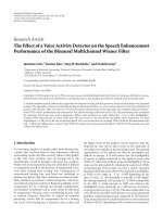
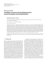
Figure 1 shows an example of the different VAD outputs
defined above. The curves obtained with these VAD meth-
ods will typically differ from each other as a function of the
specific noise and reverberation level contained in the input
signals. Compared to the binary output α
BIN
(·), the use of
soft VAD information with α
SNR
(·)andα
SP
(·) al lows the PF
0.20.40.60.811.21.4
Time (s)
1
0.5
0
0.5
1
(a)
0.20.40.60.811.21.4
Time (s)
0
0.5

1
1.5
α
BIN
α
SNR
α
SP
(b)
Figure 1: Practical example of three considered VAD methods. (a)
Input signal data. (b) Resulting VAD outputs.
to track the source in a more subtle manner. For instance, a
VA D ou t pu t v alu e 0 <α(
·) < 1effec tively indicates that the
input signals may be partly corrupted by disturbance sources,
and that the current SBF observation might not be fully accu-
rate. The PF can then take account of this fact and use more
caution when updating the particle set, and hence, when de-
termining the source location estimate. With the binary VAD
output α
BIN
(·), the source tracking process is basically turned
fully on or off based on ρ(
·) (hard decisions), which may not
be advantageous when a high level of noise and/or reverber-
ation is present. In the next section, results from experimen-
tal simulations of the PF-VAD method will determine w hich
one of these three approaches delivers the best tracking per-
formance.
6. EXPERIMENTAL RESULTS

This section presents some examples of the tracking results
obtained with the proposed PF-VAD algorithm. The various
parameters of the PF-VAD implementation were optimised
empirically and set to the following values: the number of
particles was set to N
= 50, the effective sample size thresh-
old N
thr
= 37.5, the standard deviation of the observation
density was defined as σ
Y
= 0.15 m, and the nonlinear expo-
nent was set to r
= 2. Following standard definitions (see,
e.g., [2, 3]), the PF-VAD implementation made use of the
propagation model parameters
v = 0.8m/s andβ = 10 Hz.
The VAD parameters were defined as P
FA
= 0.03 and D = 8.
The audio signals were sampled with a frequency of 16 kHz
and processed in nonoverlapping frames of L
= 256 samples
each.
8 EURASIP Journal on Advances in Signal Processing
For comparison pur poses, the performance assessment
given in this section also includes results from the SBF-PL
algorithm, a sound source tracking scheme previously pro-
posed in [2]. The SBF-PL method relies on a particle filtering
approach similar to that presented in this work, but does not

include any VAD measurements. The reader is referred to [2]
for a more detailed description of the SBF-PL implementa-
tion, and to [16] for a summary of its practical performance
results and a comparison with other tracking methods.
6.1. Assessment parameters
The experimental results make use of the following parame-
ters to assess the tracking accuracy of the considered meth-
ods. The PF estimation error for the current frame is
ε
k
=



S,k
− 

X,k


, (39)
where 
S,k
is the ground-truth source position at t ime k.In
order to assess the overall performance of the developed al-
gorithm over a given sample of audio data, the average error
is simply computed as
ε =
1
K

K

k=1
ε
k
, (40)
with K representing the total number of frames in the con-
sidered audio sample. The standard deviation parameter σ
k
,
see (26), is also used here as an overall indication of the PF
tracking p erformance in the following results presentation.
6.2. Image method simulations
The proposed PF algorithm was put to the test using syn-
thetic reverberant audio data generated using the image
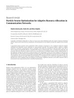
source method [20]. The results presented in this section
were obtained using audio data generated with the source
trajectory, source signal, and microphone setup depicted in
Figure 2. The dimension of the enclosure was set to 3 m
×
3m× 2.5 m, and the height of the microphones, as well as
that of the source, was defined as 1.5m.
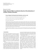
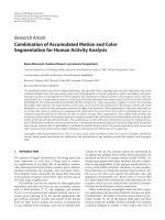
Figure 3 presents some typical results obtained with the
two considered ASLT methods (where PF-VAD uses the
speech-based VAD output α
SP
), using the setup of Figure 2
with a reverberation time T
60
≈ 0.1 s and input SNR of ap-

proximately 15 dB. This figure clearly illustrates the most sig-
nificant outcome of the PF-VAD implementation. Fusing the
VAD measurements within the PF framework effectively al-
lows the tracking algorithm to put more emphasis on the
considered dynamics model in (8) when spreading the par-
ticles during nonspeech periods, while at the same time re-
ducing the importance of the SBF observations due to the
fact that no useful information can be derived from them
when the speaker is inactive. This consequently allows the
PF to keep track of the silent target, and to resume track-
ing successfully when the speaker becomes active again. This
can be distinctly noticed with the consistent increase of the
σ
k
values for PF-VAD (Figure 3(b)) during significant gaps
in the speech signal. This specific effect originates from the
123456
Time (s)
0.2
0
0.2
(a)
00.511.522.53
x axis (m)
0
0.5
1
1.5
2
2.5

3
y axis (m)
Start
End
(b)
Figure 2: Setup for image method simulations. (a) Source signal.
(b) Microphone positions (
◦) and par abolic source trajectory.
influence of the VAD measurements on the effective sample
size parameter N
eff
. Figure 4(b) shows an example of the N
eff
values computed during one run of PF-VAD versus time. As
describedinstep3ofAlgorithm 1, the parameter N
eff
is reset
to N after the resampling stage is carried out, and the re-
sult in Figure 4 thus provides an overall view of the resam-
pling frequency. This plot demonstrates how the VAD out-
put “freezes” the N
eff
value during nonspeech periods, effec-
tively decreasing the occurrence of the particle resampling
step, which in turn leads to a spatial evolution of the particles
according to the dynamics model only.
As an important consequence of this fac t, the standard
deviation σ
k
delivered by PF-VAD effectively reflects a “true”

confidence level, that is, in keeping with the estimation accu-
racy, and can be hence directly used as an indication of the
reliability of the PF estimates. For instance, an obvious add-
on to the PF-VAD method would be to simply discard the PF
location estimates whenever σ
k
is above a predefined thresh-
old.
On the other hand, the more or less constant resampling
frequency implemented as part of the SBF-PL method pre-
cludes this desired behaviour, meaning that the particles al-
ways remain very concentrated spatially. This essentially im-
plies that during nonspeech periods, the SBF-PL particle fil-
ter continues its tracking as if the speaker was still active, and
E. A. Lehmann and A. M. Johansson 9
123456
Time (s)
1
0.5
0
0.5
1
(a)
123456
Time (s)
0
0.2
0.4
0.6
Distance (m)

Estimation error ε
k
Standard deviation σ
k
PF-VAD
(b)
123456
Time (s)
0
0.2
0.4
0.6
Distance (m)
Estimation error ε
k
Standard deviation σ
k
SPF-PL
(c)
Figure 3: Tracking result examples for two ASLT methods, for
T
60
≈ 0.1 s and SNR ≈ 15 dB. (a) Example of microphone signal.
(b) and (c) Estimation error and standard deviation for PF-VAD
and SBF-PL (results averaged over 100 simulation runs).
is hence much more likely to be driven off-track by the ef-
fects of reverberation and additive noise. An example of such
a scenario is show n in Figure 3(c), where SBF-PL loses track
of the speaker at the end of the simulation due to a significant
gap in the speech signal.

Figures 5 and 6 present the average tracking results ob-
tained for the proposed PF-VAD algorithm, as well as a
comparison with the previously developed SBF-PL method.
These plots show the average error
ε computed over a range
of input SNR values (Figure 5) and reverberation times
(Figure 6). Different T
60
values were achieved by appro-
priately setting the walls’ reflection coefficients in the im-
age method implementation. Statistical averaging was per-
formed due to the random nature of the PF implementation,
and the results depicted in these figures represent the average
over 100 simulation runs of the considered algorithms, using
the above-mentioned image method setup.
123456
Time (s)
1
0.5
0
0.5
1
(a)
123456
Time (s)
30
35
40
45
50

55
N
eff
(b)
Figure 4: Overview of the resampling frequency during one run of
PF-VAD. (a) Example of input signal used for this simulation, and
(b) effective sample size parameter N
eff
versus time (dashed line:
threshold N
thr
).
These results clearly demonstrate the superiority of the
proposed PF-VAD algorithm. The SBF-PL method consis-
tently exhibits a larger average error due to track losses oc-
curring as a result of significant gaps in the considered speech
signal (see the source signal plotted in Figure 2(a)), which the
PF-VAD implementation manages to avoid. Also, it must be
kept in mind that the PF-VAD results shown in Figures 5
and 6 correspond to the mean error
ε computed over the en-
tire length of the considered audio sample. This typically also
includes periods where the PF has a low confidence level in
its estimates. As mentioned earlier, the average performance
of PF-VAD would improve even further if tracking estimates
were discarded when σ
k
is above a predefined threshold.
In regards to a comparison of the three tested VAD
schemes with each other, it can be seen from Figures 5 and

6 that the speech-based VAD scheme α
SP
generally tends to
yield the best overall tracking performance, given the specific
test setup considered in this section. This result suggests that
the most useful information from a tracking point of view
relies more on the amount of speech present during a given
time frame, rather than the speech-to-noise ratio, which, for
instance, may become large despite a small speech signal level
in some circumstances.
6.3. Real-time implementation and real audio tracking
While the image method simulations presented in the pre-
vious section are useful to gauge the proposed algorithm’s
ability to deal with the considered ASLT problem, only a real-
time implementation, used in conjunction with real audio
signals, is able to provide a full insight into how suitable the
10 EURASIP Journal on Advances in Signal Processing
0 5 10 15 20 25
SNR (dB)
0
0.05
0.1
0.15
0.2
0.25
0.3
0.35
0.4
0.45
0.5

Mean error ε (m)
SBF-PL
PF-VAD, α
BIN
PF-VAD, α
SNR
PF-VAD, α
SP
Figure 5: Average tracking error versus input signal SNR, for T
60
≈
0.1 s (results averaged over 100 simulation runs).
00.10.20.30.40.50.6
T
60
(s)
0
0.1
0.2
0.3
0.4
0.5
0.6
0.7
Mean error ε (m)
SBF-PL
PF-VAD, α
BIN
PF-VAD, α
SNR

PF-VAD, α
SP
Figure 6: Average tracking error versus reverberation time T
60
, with
input SNR of about 20 dB (results averaged over 100 simulation
runs).
algorithm is for practical applications. Such an implementa-
tion has also been carried out in the frame of this research.
However, for the sake of conciseness, details of this imple-
mentation and of the real audio tracking results are presented
elsewhere, and only a brief review of these results is presented
here.
The PF-VAD algorithm was implemented on a standard
1.8 GHz IBM-PC running under Linux, used in conjunction
with an array of eight microphones sampled at 16 kHz. An
analysis of the algorithm showed that an implementation
with 100 particles results in a computational complexity of
71.5 M floating-point operations per second (FLOPS), re-
sulting in a CPU load during execution of about 5%. These
results hence demonstrate the suitability of the PF-VAD
method for real-time processing on low-power embedded
systems using all-purpose hardware and software. Full details
of this real-time implementation can be found in [21].
A f ull tracking performance assessment of the PF-VAD
algorithm was also conducted using samples of real audio
data, recorded in a reverberant environment. A microphone
array, similar to that shown in Figure 2,wassetupinaroom
with dimensions 3.5m
× 3.1m × 2.2m and a practical re-

verberation time of T
60
≈ 0.3 s (frequency-averaged up to
24 kHz). The experimental results using this pra ctical setup
are reported in [22], and confirm the improved efficiency of
PF-VAD compared to SBF-PL when used in real-world cir-
cumstances.
7. CONCLUSION AND FUTURE WORK
This work is concerned with the problem of tracking a
human speaker in reverberant and noisy environments by
means of an ar ray of acoustic sensors. We der ived a PF-based
method that integrates VAD measurements at a low level in
the statistical algorithm framework. Provided the dynamics
of the considered acoustic source are properly modeled, the
proposed PF-VAD method greatly reduces the likelihood of
a complete track loss during long silence gaps in the speech
signal. The proposed algorithm hence provides an improved
tracking performance for real-world implementations com-
pared to previously derived PF methods. As a further result
of the proposed implementation, the standard deviation of
the particle set can now be used as a reliable indication of
the filter’s own estimation accuracy. The obvious limitation
inherent to the current developments is that only one sin-
glespeakercanbetrackedatatime.Thisworkwillhowever
serve as a basis for further research on the problem of multi-
ple speaker tracking using the principle of microphone array
beamforming.
ACKNOWLEDGMENTS
The authors would like to thank the anonymous reviewers
for their valuable suggestions and comments, as well as Alan

Davis for the help provided in regards to the VAD s cheme
used in this paper. This work was supported by National
ICT Australia (NICTA) and the Australian Research Coun-
cil (ARC) under Grant no. DP0451111. NICTA is funded by
the Australian Government’s Department of Communica-
tions, Information Technology and the Arts, the Australian
Research Council through Backing Australia’s Ability, and
the ICT Centre of Excellence programs.
REFERENCES
[1] S. Gannot and T. G. Dvorkind, “Microphone array speaker lo-
calizers using spatial-temporal information,” EURASIP Jour-
nal on Applied Signal Processing, vol. 2006, Article ID 59625,
17 pages, 2006.
E. A. Lehmann and A. M. Johansson 11
[2] D. B. Ward, E. A. Lehmann, and R. C. Williamson, “Particle
filtering algorithms for tracking an acoustic source in a rever-
berant environment,” IEEE Transactions on Speech and Audio
Processing, vol. 11, no. 6, pp. 826–836, 2003.
[3] J. Vermaak and A. Blake, “Nonlinear filtering for speaker
tracking in noisy and reverberant environments,” in Proceed-
ings of IEEE International Conference on Acoustics, Speech and
Signal Processing (ICASSP ’01), vol. 5, pp. 3021–3024, Salt Lake
City, Utah, USA, May 2001.
[4] I. Potamitis, H. Chen, and G. Tremoulis, “Tracking of multi-
ple moving speakers with multiple microphone arrays,” IEEE
Transactions on Speech and Audio Processing,vol.12,no.5,pp.
520–529, 2004.
[5] T. G. Dvorkind and S. Gannot, “Speaker localization ex-
ploiting spatial-temporal information,” in Proceedings of the
International Workshop on Acoustic Echo and Noise Control

(IWAENC ’03), pp. 295–298, Kyoto, Japan, September 2003.
[6] D. Bechler, M. Grimm, and K. Kroschel, “Speaker tracking
with a microphone array using Kalman filtering,” Advances in
Radio Science, vol. 1, pp. 113–117, 2003.
[7] J. Chen, L. Shue, and W. Ser, “A new approach for speaker
tracking in reverberant environment,” Signal Processing,
vol. 82, no. 7, pp. 1023–1028, 2002.
[8] Y. Huang, J. Benesty, and G. W. Elko, “Passive acoustic source
localization for video camera steering,” in Proceedings of the
IEEEInternationalConferenceonAcoustics,SpeechandSignal
Processing (ICASSP ’00), vol. 2, pp. 909–912, Istanbul, Turkey,
June 2000.
[9] S. Doclo and M. Moonen, “Robust adaptive time delay estima-
tion for speaker localization in noisy and reverberant acoustic
environments,” EURASIP Journal on Applied Signal Processing,
vol. 2003, no. 11, pp. 1110–1124, 2003.
[10] X. Sheng and Y. H. Hu, “Sequential acoustic energy based
source localization using particle filter in a distributed sensor
network,” in Proceedings of the IEEE International Conference
on Acoustics, Speech and Signal Processing (ICASSP ’04), vol. 3,
pp. 972–975, Montreal, Qu
´
ebec, Canada, May 2004.
[11] J. C. Chen, K. Yao, and R. E. Hudson, “Acoustic source localiza-
tion and beamforming: theory and practice,” EURASIP Jour-
nal on Applied Signal Processing, vol. 2003, no. 4, pp. 359–370,
2003.
[12] A. Davis, S. Nordholm, and R. Togneri, “Statistical voice activ-
ity detection using low-variance spectrum estimation and an
adaptive threshold,” IEEE Transactions on Audio, Speech and

Language Processing, vol. 14, no. 2, pp. 412–424, 2006.
[13] B. Anderson and J. Moore, Optimal Filtering,Dover,New
York, NY, USA, 2005.
[14] M. S. Arulampalam, S. Maskell, N. Gordon, and T. Clapp, “A
tutorial on particle filters for online nonlinear/non-Gaussian
Bayesian tracking,” IEEE Transactions on Signal Processing,
vol. 50, no. 2, pp. 174–188, 2002.
[15] N.J.Gordon,D.J.Salmond,andA.F.M.Smith,“Novelap-
proach to nonlinear/non-Gaussian Bayesian state estimation,”
IEE Proceedings, F: Radar and Signal Processing, vol. 140, no. 2,
pp. 107–113, 1993.
[16] E. A. Lehmann, D. B. Ward, and R. C. Williamson, “Experi-
mental comparison of particle filtering algorithms for acous-
tic source localization in a reverberant room,” in Proceedings of
the IEEE International Conference on Acoustics, Speech, and Sig-
nal Processing (ICASSP ’03), vol. 5, pp. 177–180, Hong Kong,
April 2003.
[17] C. H. Knapp and G. C. Carter, “The generalized correlation
method for estimation of time delay,” IEEE Transactions on
Acoustics, Speech, and Signal Processing, vol. 24, no. 4, pp. 320–
327, 1976.
[18] R. Waterhouse, “Statistical properties of reverberant sound
fields,” Journal of the Acoustical Society of America, vol. 43,
no. 6, pp. 1436–1444, 1968.
[19] S. Haykin, Communication Systems, John Wiley & Sons, New
York, NY, USA, 3rd edition, 1994.
[20] J. B. Allen and D. A. Berkley, “Image method for efficiently
simulating small-room acoustics,” Journal of the Acoustical So-
ciety of America, vol. 65, no. 4, pp. 943–950, 1979.
[21] A. M. Johansson, E. A. Lehmann, and S. Nordholm, “Real-

time implementation of a particle filter with integrated voice
activity detector for acoustic speaker tracking,” in Proceedings
of the IEEE Asia Pacific Conference on Circuits and Systems
(APCCAS ’06), Singapore, December 2006.
[22] E. A. Lehmann and A. M. Johansson, “Experimental perfor-
mance assessment of a particle filter with voice activity data
fusion for acoustic speaker tracking,” in Proceedings of the
7th IEEE Nordic Signal Processing Symposium (NORSIG ’06),
Reykjavik, Iceland, June 2006.
Eric A. Lehmann graduated in 1999 from
the Swiss Federal Institute of Technology
in Zurich (ETHZ), Switzerland, with a
Diploma in elect rical engineering (Master
equivalent). He received the M.Phil. and
Ph.D. degrees, both in electrical engineer-
ing, from the Australian National Univer-
sity (Canberra) in 2000 and 2004, respec-
tively. After working as a Research Engineer
for National ICT Australia (NICTA) in Can-
berra, he now holds a research position with the Western Aus-
tralian Telecommunications Research Institute (WATRI) in Perth,
Australia. His current scientific interests include acoustics, signal
and speech processing, microphone arrays, and Bayesian estima-
tion and tracking, with particular emphasis on the application of
sequential Monte Carlo methods (particle filters).
Anders M. Johansson wasbornonFebru-
ary 10, 1974, in Sweden. He studied Tele-
communications and Signal Processing at
the Blekinge Technical University and re-
ceived a Master’s degree in electrical en-

gineering in 2000. He held the posi-
tion of Research Engineer at the Aus-
tralian Telecommunications Research Insti-
tute from 2000 to 2002, and at the West Aus-
tralian Telecommunications Research Insti-
tute, from 2002 to present, developing real-time software for re-
search in the field of acoustic sig nal processing. His main fields
of interest include acoustic source localisation, blind signal sepa-
ration, real-time signal processing, and acoustics.