Báo cáo hóa học: " Research Article Calibrating Distributed Camera Networks Using Belief Propagation" pptx

Hindawi Publishing Corporation
EURASIP Journal on Advances in Signal Processing
Volume 2007, Article ID 60696, 10 pages
doi:10.1155/2007/60696
Research Article
Calibrating Distributed Camera Networks Using
Belief Propagation
Dhanya Devarajan and Richard J. Radke
Department of Electrical, Computer, and Systems Engineering, Rensselaer Polytechnic Institute,
Troy, NY 12180, USA
Received 4 January 2006; Revised 10 May 2006; Accepted 22 June 2006
Recommended by Deepa Kundur
We discuss how to obtain the accurate and globally consistent self-calibration of a distributed camera network, in which camera
nodes with no centralized processor may be spread over a wide geographical area. We present a distributed calibration algorithm
based on belief propagation, in which each camera node communicates only with its neighbors that image a sufficient number of
scene points. The natural geometry of the system and the formulation of the estimation problem give rise to statistical dependencies
that can be efficiently leveraged in a probabilistic framework. The camera calibration problem poses several challenges to informa-
tion fusion, including overdetermined parameterizations and nonaligned coordinate systems. We suggest practical approaches to
overcome these difficulties, and demonstrate the accurate and consistent performance of the algorithm using a simulated 30-node
camera network with varying levels of noise in the correspondences used for calibration, as well as an experiment with 15 real
images.
Copyright © 2007 D. Devarajan and R. J. Radke. This is an open access article distributed under the Creative Commons
Attribution License, which permits unrestricted use, distribution, and reproduction in any medium, provided the original work is
properly cited.
1. INTRODUCTION
Camera calibration up to a metric frame based on a set
of images acquired from multiple cameras is a central is-
sue in computer vision. While this problem has been ex-
tensively studied, most pr ior work assumes that the cali-
bration problem is solved at a single processor after the
images have been collected in one place. This assumption

is reasonable for much of the early work on multicam-
era vision in which all the cameras are in the same room
(e.g., [1, 2]). However, recent developments in w i reless sen-
sornetworkshavemadefeasibleadistributed came ra net -
work, in w hich cameras and processing nodes may be spread
over a wide geographical area, w ith no centralized pro-
cessor and limited ability to communicate a large amount
of information over long distances. We will require new
techniques for calibrating distributed camera networks—
techniques that do not require the data from all cameras
to be stored in one place, but ensure that the distributed
camera calibration estimates are both a ccurate and globally
consistent across the network. Consistency is especially im-
portant, since the camera network is presumably deployed
to perform a high-level vision task such as tracking and
triangulation of an object as it moves through the field of
cameras.
In this paper, we address the calibration of a distributed
camera network using belief propagation (BP), an inference
algorithm that has recently sparked interest in the sensor net-
working community. We describe the belief propagation al-
gorithm, discuss se veral challenges that are unique to the
camera calibration problem, and present practical solutions
to these difficulties. For example, both local and global col-
lections of camera parameters can only be specified up to
unknown similarity transformations, which requires itera-
tive reparameterizations not typical in other BP applications.
We demonstrate the accurate and consistent camera network
calibration produced by our algorithm on a simulated cam-
era network with no constraints on topology, as well as on a

set of real images. We show that the inconsistency in camera
localization is reduced by factors of 2 to 6 after BP, while still
maintaining high accuracy.
The paper is organized as follows. Section 2 reviews dis-
tributed inference methods, especial ly those related to sen-
sor networks applications. Section 3 provides a brief descrip-
tion of the distributed procedure we use to initialize the
camera calibration estimates. Section 4 describes the belief
2 EURASIP Journal on Advances in Signal Processing
propagation algorithm in a general way, and Section 5 goes
into detail on challenging aspects of the inference algorithm
that arise when dealing with camera calibration. Section 6
analyzes the performance of the algorithm in terms of both
calibration accuracy and the ultimate consistency of esti-
mates. Finally, Section 7 concludes the paper and discusses
directions for future work.
2. RELATED WORK
Since our calibration algorithm is based on information fu-
sion, here we briefly review related work on distributed in-
ference. Traditional decentralized navigation systems use dis-
tributed Kalman filtering [3] for fusing parameter estimates
from multiple sources, by approximating the system with lin-
ear models for state transitions and interactions between the
observed and hidden states. Subsequently, extended Kalman
filtering was developed to accommodate for nonlinear inter-
actions [4]. However, the use of distributed Kalman filtering
requires a tree network topology [5], which is generally not
appropriate for the graphical model for camera networks dis-
cussed in Section 4.
Recently, the sensor networking community has seen a

renewed interest in message-passing schemes on graphical
networks with arbitrary topologies, such as belief propaga-
tion [6]. Such algorithms rely on local interactions between
adjacent nodes in order to infer posterior or marginal den-
sities of parameters of interest. For networks without cycles,
inferences (or beliefs) obtained using BP are known to con-
verge to the correct densities [7]. However, for networks with
cycles, BP might not converge, and even if it does, conver-
gence to the correct densities is not always guaranteed [6, 7].
Regardless, several researchers have reported excellent empir-
ical performance running loopy belief propagation (LBP) in
various applications [6, 8, 9]; turbo decoding [10]isonesuc-
cessful example. Networks in which parameters are modeled
with Gaussian densities are known to converge to the right
means, even if the covariances are incorrect [11, 12].
In the computer vision literature, message-passing
schemes using pairwise Markov fields have generally been
discussed in the context of image segmentation [13]and
scene estimation [14]. Other recent vision applications of be-
lief propagation include shape finding [15], image restora-
tion [16], and tracking [17]. In vision applications, the pa-
rameters of interest usually represent pixel labels or intensity
values. Similarly, several researchers have investigated dis-
tributed inference in the context of ad hoc sensor networks,
for example, [18, 19]. The variables of interest in such cases
are usually scalars such as temperature or light intensity. In
either case, applications of BP frequently operate on prob-
ability mass functions, which are usually straightforward to
work with. In contrast, the state vector at each node in our
problem is a high- (e.g., 40) dimensional continuous random

variable.
The state of the art in distributed inference in sensor net-
works is represented by the work of Paskin and Guestrin
[20], Paskin et al. [21], and Dellaert et al. [22]. In [20],
Paskin and Guestrin presented a message-passing algorithm
for distributed inference that is more robust than belief prop-
agation in several respects, which was applied to several sen-
sor networking scenarios in [21]. In [23], Funiak et al. ex-
tended this approach to camera calibration based on simul-
taneous localization and tracking (SLAT) of a moving object.
In [22], Dellaert et al. applied an alternate but related ap-
proach for distributed inference to simultaneous localization
and mapping (SLAM) in a planar environment.
In this paper, we focus on distributed camera calibration
in 3D, which presents several challenges not found in SLAM
or networks of scalar/discrete state variables. While we dis-
cuss belief propagation here because of its widespread use
and straightforward explanation, our algorithm could cer-
tainly benefit from the more sophisticated distributed infer-
ence algorithms mentioned above.
3. DISTRIBUTED INITIALIZATION
We assume that the camera network contains M nodes, each
representing a perspective camera described by a 3
×4matrix
P
i
:
P
i
= K

i
R
T
i

I −C
i

. (1)
Here, R
i
∈ SO(3) and C
i
∈ R
3
are the rotation matrix and
optical center comprising the external camera parameters. K
i
is the intrinsic parameter matrix, which we assume here can
be written as diag( f
i
, f
i
,1),where f
i
is the focal length of the
camera. (Additional parameters can be added to the camera
model, e.g., principal points or lens distortion, as the situa-
tion warrants.)
Each camera images some subset of a set of N scene

points
{X
1
, X
2
, , X
N
}∈R
3
. This subset for camera i is de-
scribed by S
i
⊂{1, , N}. The projection of X
j
onto P
i
is
given by u
ij
∈ R
2
for j ∈ S
i
:
λ
ij

u
ij
1


=
P
i

X
j
1

,(2)
where λ
ij
is called the projective depth [24].
We define a g raph G
= (V,E) on the camera network
called the vision graph, where V is the set of vertices (i.e.,
the cameras in the network) and an edge is present in E if
two camera nodes observe a sufficient number of the same
scene points from different perspectives (more precisely, an
edge exists if a stable, accurate estimate of the epipolar ge-
ometry can be obtained). We define the neighbors of node i
as N( i)
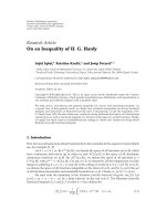
={j ∈ V | (i, j) ∈ E}. A sample camera network
and its corresponding vision graph are sketched in Figure 1.
A companion article in this special issue describes our ap-
proach to obtaining the vision graph for a collection of real
images [25].
To obtain a distributed initial estimate of the camera pa-
rameters, we use the algorithm we previously described in
[26],whichroughlyoperatesasfollowsateachnodei.

(1) Estimate a projective reconstruction [24] based on the
common scene points shared by i and N(i) (these
points are cal led the “nucleus”).
D. Devarajan and R. J. Radke 3
1
2
3456
7
8
(a)
1
2
3
4
56
7
8
(b)
Figure 1: (a) A snapshot of the instantaneous state of a camera net-
work, indicating the fields of view of eight cameras, (b) the associ-
ated vision graph.
(2) Estimate a metric reconstruction based on the projec-
tive cameras [27].
(3) Triangulate scene points not in the nucleus using the
calibrated cameras [28].
(4) Use RANSAC [29]torejectoutlierswithlargerepro-
jection error, and repeat until the reprojection error
for all points is comparable to the assumed noise level
in the correspondences.
(5) Use the resulting st ructure-from-motion estimate as

the starting point for full bundle adjustment [30]. That
is, if u
jk
represents the projection of

X
i
k
onto

P
i
j
, then
the nonlinear cost function that is minimized at each
cluster i is given by
min
{P
i
j
}, j∈{i,N(i)}
{
X
i
k
}, k∈∩S
j

j


k

u
jk
− u
jk

T
Σ
−1
jk

u
jk
− u
jk

,(3)
where Σ
jk
is the 2×2 covariance matrix associated with
the noise in the image p oint u
jk
. The quantity inside
the sum is called the Mahalanobis distance between
u
jk
and u
jk
.

If the local calibration at a node fails for any reason, a
camera estimate is acquired from a neighboring node prior
to bundle adjustment. At the end of this initial calibration,
each node has estimates of its own camera parameters P
i
i
,as
well as those of its neighbors in the vision graph P
i
j
, j ∈ N(i).
A major issue is that even when the local calibrations are
reasonably accurate, the estimates of the same parameter at
different nodes will generally be inconsistent. For example, in
Figure 1(b), cameras 1 and 5 will disagree on the location of
camera 8, since the parameters at 1 and 5 are estimated with
almost entirely disjoint data. As mentioned above, consis-
tency is critical for accurate performance on higher-level v i-
sion tasks. A na
¨
ıve approach to obtaining consistency would
be to simply collect and average the inconsistent estimates
of each parameter. However, this is only statistically optimal
when the joint covariances of all the parameter estimates are
identical, which is never the case. In Section 4, we show how
parameter estimates can be effectively combined in a prob-
abilistic framework using pairwise Markov random fields,
paying proper attention to the covariances.
4. BELIEF PROPAGATION FOR VISION GRAPHS
Let Y

i
represent the true state vector at node i that collects the
parameters of that node’s camera matrix P
i
i
as well as those
of its neighbors P
i
j
, j ∈ N(i), and let Z
i
be the noisy “ob-
servation” of Y
i
that comes from the local calibration pro-
cess. That is, the observations arise out of local bundle ad-
justment on the image projections of common scene points
{u
jk
| j ∈{i, N(i)}, k ∈ S
i
} that are used as the basis for the
initial calibration. Our goal is to estimate the true state vector
Y
i
at each node given all the observations by calculating the
marginal
p

Y

i
| Z
1
, , Z
M

=

{Y
j
, j=i}
p

Y
1
, , Y
M
| Z
1
, , Z
M

dY
j
.
(4)
Recently, belief propagation has proven effective for
marginalizing state variables based on local message pass-
ing; we briefly describe the technique below. According to
the Hammersley-Clifford theorem [31, 32], a joint density

is factorizable if and only if it satisfies the pairwise Markov
property,
p

Y
1
, Y
2
, , Y
M

∝

i∈V
φ
i

Y
i


(i, j)∈E
ψ
ij

Y
i
, Y
j


,(5)
where φ
i
represents the belief (or evidence) potential at node
i,andψ
ij
is a compatibility potential relating each pair of
nodes (i, j)
∈ E.Pearl[7] later proved that an inference on
this factorized model is equivalent to a message-passing sys-
tem, where each node updates its belief by obtaining infor-
mation or messages from its neighbors. This process is what
is generally referred to as belief propagation. The marginal-
ization is then achieved through the update equations
m
t
ij

Y
j

∝

Y
i
ψ

Y
i
, Y

j

φ

Y
i


k∈N(i)\ j
m
t−1
ki

Y
i

dY
i
,
b
t
i

Y
i

∝
φ

Y

i


j∈N(i)
m
t
ji

Y
i

,
(6)
where m
t
ij
is the message that node i transmits to node j at
time t,andb
t
i
is the belief at node i about its state, which is the
approximation to the required marginal density p(Y
i
)attime
t. This algorithm is also called the sum-product algorithm.
4 EURASIP Journal on Advances in Signal Processing
1
2
3456
7

8
m
21
( P
2
1
, P
2
2
, P
2
3
)
m
31
( P
3
1
, P
3
2
, P
3
3
)
m
81
( P
8
1

, P
2
8
, P
8
8
)
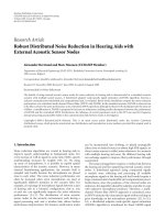
Figure 2: An intermediate stage of message passing . The P
j
i
indicate
the camera parameters that are passed between nodes.
In our problem, the joint density in (4) can be expressed
as
p

Y
1
, Y
2
, , Y
M
| Z
1
, , Z
M

∝
p


Y
1
, Y
2
, , Y
M
, Z
1
, , Z
M

(7)
=

i∈V
p

Z
i
| Y
i


(i, j)∈E
p

Y
i
, Y
j


. (8)
Here, Z
i
is observed and hence the likelihood func tion p(Z
i
|
Y
i
) is a function of Y
i
. Similar factorizations of the joint den-
sity are common in decoding systems [33].
p(Y
i
, Y
j
) encapsulates the constraints between the vari-
ables Y
i
and Y
j
. That is, the random vectors Y
i
and Y
j
may
share some random variables that must agree. We enforce
this constraint by defining binary selector matrices C
ij

based
on the vision graph as follows. Let M
ij
be the number of cam-
era parameters that Y
i
and Y
j
have in common. Then C
ij
is
a binary M
ij
×|Y
i
| matrix such that C
ij
Y
i
selects and orders
these common variables. Then we assume
P

Y
i
, Y
j

∝ δ


C
ij
Y
i
− C
ji
Y
j

,(9)
where δ(x)is1whenallentriesofx are 0 and 0 otherwise.
The joint density (9) makes the implicit assumption of a uni-
form prior over the true state variables; that is, it only en-
forces that common par ameters match. If available, prior in-
formation about the density of the state var iables could be
directly incorporated into (9), and might result in improved
performance compared to the uniform density assumption.
Therefore, we can see that (8) is in the desired form of
(5), identifying
φ
i

Y
i

∝
p

Z
i

| Y
i

,
ψ
ij

Y
i
, Y
j

∝
δ

C
ij
Y
i
− C
ji
Y
j

.
(10)
Based on this factorization, it is possible to perform the
belief propagation directly on vision graph edges using the
update (6). Figure 2 represents one step of the message pass-
ing, indicating the actual camera parameters that are in-

volved in each message.
For Gaussian densities, the BP equations reduce to pass-
ing and u pdating the first two moments of each Y
i
.Letμ
i
represent the mean of Y
i
,andΣ
i
the corresponding covari-
ance matrix. Node i receives estimates μ
j
i
and Σ
j
i
from each
of its neighbors j
∈ N(i). Then the update (6)reducesto
minimizing the sum of the KL divergences between the up-
dated Gaussian density and each incoming Gaussian density.
Therefore, the belief update reduces to the well-known equa-
tions [4]
μ
i
i
←−

Σ

−1
i
+

j∈N(i)

Σ
j
i

−1

−1

Σ
−1
i
μ
i
+

j∈N(i)

Σ
j
i

−1
μ
j

i

,
Σ
i
i
←−

Σ
−1
i
+

j∈N(i)

Σ
j
i

−1

−1
.
(11)
We note that (11) can be iteratively calculated in pairwise
computations, instead of being computed in batch, and that
this pairwise fusion is invariant to the order in which the es-
timates arrive.
Although (11) assumes that the dimensions of μ
j

i
are the
same for all j
∈ N(i), this is usually not the case in prac-
tice, since the message sent from node i to node j would be a
function of the subset C
ij
Y
j
rather than Y
j
. This can be easily
dealt with by setting the entries of the mean and inverse co-
variance matrix corresponding to the parameters not in the
subset to 0. In this way, the dimensions of the means and
variances all agree, but the missing variables play no role in
the fusion.
We obtain the mean and covariance of the assumed
Gaussian density p(Z
i
| Y
i
) based on forward covariance
propagation from bundle adjustment. That is, the covari-
ances of the noise in the image correspondences used for
bundle adjustment are propagated through the bundle ad-
justment cost functional (3) to obtain a covariance on the
structure-from-motion parameters at each node [34]. Since
we are predominantly interested in localizing the camera net-
work, we marginalize out the reconstructed 3D structure to

obtain covariances of the camera parameters alone.
5. CHALLENGES FOR CAMERA CALIBRATION
The BP framework as described above is generally applicable
to many information fusion applications. However, when the
beliefs represent distributed estimates of camer a parameters,
there are several additional difficulties, which we discuss in
this section. These issues include the following.
(1) Minimal parameterizations. Even if each camera ma-
trix is parameterized minimally at node i (i.e., 1 parameter
for focal length, 3 parameters for camera center, 3 parame-
ters for rotation matrix), there are still 7 degrees of freedom
corresponding to an unknown similarity transformation of
all cameras in Y
i
. Without modification, covariance matri-
ces in (11) have null spaces of dimension 7 and cannot be
inverted.
(2) Frame alignment. Sinceweassumetherearenoland-
marks in the scene with known 3D positions, the camera
motion parameters can be estimated only up to a similar-
ity transformation, and this unknown similarity transforma-
tion will differ from node to node. The estimates Y
i
i
and
Y
j
i
, j ∈ N(i), must be brought to a common coordinate sys-
tem before every fusion step.

D. Devarajan and R. J. Radke 5
(3) Incompatible estimates. The covariances of each Y
i
are
obtained from independent processes, and may produce an
unreliable result in the direct implementation of (11).
We address each of the above issues in the following sec-
tions.
5.1. Minimal parametrization
We minimally parameterize each camera matrix P in Y
i
by
7 parameters: its focal length f , its camera center (x, y, z),
and the axis-angle parameters (a, b, c) representing its rota-
tion matrix. If
|{i, N(i)}| = n
i
, then the set of 7n
i
parameters
is not a minimal parametrization of the joint Y
i
, since the
cameras can only be recovered up to a similarity transforma-
tion. Without modification, the covariance matrices of the Y
i
estimateswillbesingular.
Since Y
i
always includes an estimate of P

i
,weapplyarigid
motion so that P
i
is fixed as K
i
[I 0] with K
i
= diag( f
i
, f
i
,1).
This eliminates 6 degrees of freedom. The remaining scale
ambiguity can be eliminated by fixing the distance between
camera i and one of its neighbors (say, node B
i
); usually we
set the distance of camera i to its lowest-numbered neighbor
to be 1, which means that the camera center of B
i
can be pa-
rameterized by only two spherical angles (θ, φ). We call this
normalization the basis for node i,orB
i
.Thus,Y
i
is mini-
mally parameterized by a set of 7(n
i

− 1) parameters:
Y
i
=

f
i
, f
B
i
, θ
B
i
, φ
B
i
, a
B
i
, b
B
i
, c
B
i
,

f
k
, x

k
, y
k
, z
k
, a
k
, b
k
, c
k
, k ∈ N(i)\

i, B
i

.
(12)
The nonsingular covariance of p(Z
i
| Y
i
) in this basis can
be obtained by forward covariance propagation as descr ibed
in Section 4.
5.2. Frame alignment
While we have a minimal parameterization at each node,
each node’s estimate is in a different basis. In order to fuse es-
timates from neighboring nodes, the parameters must be in
the same frame- that is, they must share the same basis cam-

eras. In the centralized case, we could easily avoid this prob-
lem by initially aligning all the cameras in the network to a
minimally parametrized common frame (e.g., by registering
their reconstructed scene points and specifying a gauge for
the structure-from-motion estimate [35]). However, in the
distributed case, it is not clear what would constitute an ap-
propriate gauge, how it could be estimated in a distributed
manner, how each camera could efficiently be brought to the
gauge, how the gauge should change over time, and so on.
A natural approach that avoids the problem of global
gauge fixing is to align the estimates of Y
i
to the basis B
i
prior
to each fusion at node i. A subtle issue is that in this case, the
resulting covariance matrices can become singular. This is il-
lustrated by the example in Figure 3. Consider the message to
be sent from 4 to 3. The basis at 3 is formed by cameras
{3, 1},
and the basis at 4 is formed by cameras
{4, 2}.If4changesits
basis to
{3, 1}, this is a reparameterization of its data from
14 to 15 parameters (i.e., initially we have 1 parameter for
1
2
3
4
Figure 3: Example in which the wrong method of frame alignment

can introduce singularities into the covariance matrix.
camera 4, 6 parameters for camera 2, and 7 parameters for
camera 3. After reparameterization, we would have 7 param-
eters for camera 4, 1 parameter for camera 3, and 7 param-
eters for camera 2), which introduces singularity in the new
covariance matrix. To avoid this problem, we use the follow-
ing protocol for every j
∈ N(i).
(1) Define the basis B
ij
as the one in which P
i
= K
i
[I 0]
and the camera center of P
j
has C
j
=1.
(2) Changebothnodesi and j to basis B
ij
.
(3) Update the messages and belief potentials using (6).
(4) Change the basis of the updated density at j to B
i
.
We note that every basis change requires a transformation
of the covariance using the Jacobian of the transformation.
While this Jacobian might have hundreds of elements (a 40

×
40 Jacobian is typical), it is also sparse, and most entries can
be computed analytically, except for those involving pairs of
axis-angle parameters.
5.3. Incompatible estimates
The covariances that are merged at each step come from in-
dependent processes. Towards convergence of BP, the entries
of the covariance matrices become very small. When the vari-
ances are too small (which can be detected using a threshold
on the determinant of the covariance matrix), the informa-
tion matrix (i.e., the inverse of the covariance matrix) has
very large entries and creates numerical difficulties in imple-
menting (6). At this point, we make the alternate approxima-
tion that

Σ
j
i
is a block-diagonal matrix containing no cross-
terms between cameras, w i th the current per-camera covari-
ance estimates along the diagonal. This block-diagonal co-
variance matrix is sure to be positive definite.
6. EXPERIMENTS AND RESULTS
We studied the performance of the algorithm with both sim-
ulated and real data. We judge the algorithm’s performance
by evaluating the consistency of the estimated camera pa-
rameters throughout the network both before and after BP.
For simulated data, we also compare the accuracy of the al-
gorithm before and after BP with centralized bundle adjust-
ment. On one hand, we do not expect a large change in

6 EURASIP Journal on Advances in Signal Processing
110
0
110
(m)
110
0
110
0
80
(m)
(m)
(a)
1
2
3
4
5
6
7
89
10
11
12
13
14
15
16
17
18

19
20
21
22
23
24
25
26
27
28
29
30
(b)
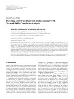
Figure 4: (a) The field of view of each of the simulated cameras.
Focal lengths have been exaggerated, (b) the corresponding vision
graph.
accuracy. The independently computed initial estimates are
already reasonably good, and BP diffuses the error from less
accurate nodes throughout the network. On the other hand,
we expect an increase in the consistency of the estimates,
since our main goal in applying BP is to obtain a distributed
consensus about the joint estimate.
6.1. Simulated experiment
We constructed a simulated scene consisting of 30 cam-
eras surveying four simulated (opaque) structures of varying
heights. The cameras were placed randomly on an elliptical
band around the “buildings.” T he dimensions of the config-
uration were chosen to model a reasonable real-world scene.
The buildings had square bases 20 m on a side and are 2 m
apart. The cameras have a pixel size of 12 μm, a focal length

of 1000 pixels, and a field of view of 600
× 600 pixels. The
nearest camera was at
≈ 88 m and the farthest at ≈ 110 m
from the scene center. Figure 4(a) illustrates the setup of the
cameras and scene.
4000 scene points were uniformly distributed along the
walls of the buildings and imaged by the 30 cameras, tak-
ing into account occlusions. The vision graph for the con-
figuration is illustrated in Figure 4(b). The projected points
were then perturbed by zero-mean Gaussian random noise
with standard deviations of 0.5, 1, 1.5, and 2 pixels for 10
realizations of noise at each level. The initial calibration
(camera parameters plus covariance) was computed using
the distributed algorithm described in Section 3; the cor-
respondences and vision graph are assumed known (since
there are no actual images in which to detect correspon-
dences). Belief propagation was then performed on the ini-
tialized network as described in Sections 4 and 5. The algo-
rithm converges when there are no further changes in the be-
liefs; in our experiments we used the convergence c riterion
Y
t
i
− Y
t−1
i
/Y
t−1
i

 < 0.001. In our experiments, the num-
berofBPiterationsrangedfrom4to12.
The accuracy of the estimated parameters, both before
and after BP, is reported in Ta ble 1.Wefirstalignedeachnode
to the known ground truth by estimating a similarity trans-
formation based on corresponding camera matrices. The er-
ror metrics for focal lengths, camera centers, and camera ori-
entations are computed as
d

f
1
, f
2

=




1 −
f
1
f
2




, (13)

d

C
1
, C
2

=


C
1
− C
2


, (14)
d

R
1
, R
2

=
2

1 − cos θ
12
, (15)

where θ
12
is the relative angle of rotation between rotation
matrices R
1
and R
2
. Table 1 reports the mean of each statis-
tic over the 10 random realizations of noise at each level. As
Tab le 1 shows, there is little change in the relative accuracy of
the network calibration before and after BP (in fact, the accu-
racy of camera centers and orientations is slightly worse after
BP in noisy cases, and the accuracy of focal lengths is slightly
better). However, the accuracy is quite comparable with that
of centralized bundle adjustment with a worst-case camera
center error of 56 cm versus 44 cm for the 2-pixel noise level
(recall the scene is 220 m wide).
The consistency of the estimated parameters, both be-
fore and after BP, is reported in Tabl e 2.Foreachnodei,we
aligned each neighbor j
∈ N(i)tobasisB
i
, and scaled the
dimensions of the result to agree with ground truth. We then
measured the consistency of all estimates of f
j
i
, C
j
i

,andR
j
i
by
computing the standard deviation of each metric (13)–(15),
using f
i
i
, C
i
i
, R
i
i
as a reference. The mean of the deviations
for each type of par ameter over all the nodes was computed,
and averaged over the 10 random realizations of noise at e ach
level.
As Tabl e 2 shows, the inconsistency of the camera param-
etersbeforeandafterBPisreducedbyfactorsofapproxi-
mately 2 to 4, with increasing improvement at higher noise
levels. Higher-level vision and sensor networking algorithms
could definitely benefit from the accurate, consistent local-
ization of the nodes, which was obtained in a completely dis-
tributed framework.
D. Devarajan and R. J. Radke 7
Table 1: Summary of the calibration accuracy. C
err
is the average absolute error in camera centers in cm (relative to a scene width of 220 m).
θ

err
is the average orientation error between rotation matri ces given by (15). f
err
is the average focal length error as a relative fraction.
Noise level Network C
err
θ
err
f
err
σ (pixels) state (cm)
Initialization 14.21.3e-3 0.0035
0.5Convergence13.91.5e-3 0.0029
Centralized bundle 12.30.9e-3 0.0015
Initialization 24.22.5e-3 0.0064
1Convergence22.92.3e-3 0.0051
Centralized bundle 24.31.7e-3 0.0031
Initialization 43.34.2e-3 0.0129
1.5Convergence44.24.0e-3 0.0081
Centralized bundle 41.82.8e-3 0.0052
Initialization 48.55.5e-3 0.0144
2Convergence55.74.5e-3 0.0115
Centralized bundle 43.64.2e-3 0.0064
Table 2: Summary of the calibration consistency. C
sd
is the average standard deviation of error in camera centers in cm (relative to a scene
width of 220 m). θ
sd
is the average standard deviation of orientation error between rotation matrices given by (15). f
sd

is the average standard
deviation of focal length error.
Noise level Network C
sd
θ
sd
f
sd
σ (pixels) state (cm)
Initialization 20.91.6e-3 0.0029
0.5Convergence11.39.8e-3 0.0016
Improvement factor 1.91.71.8
Initialization 31.72.9e-3 0.0025
1Convergence11.81.2e-3 0.0011
Improvement factor 2.72.42.7
Initialization 58.44.6e-3 0.0056
1.5Convergence16.82.1e-3 0.0018
Improvement factor 3.52.23.1
Initialization 63.46.2e-3 0.0079
2Convergence15.51.6e-3 0.0021
Improvement factor 4.13.83.8
6.2. Real experiment
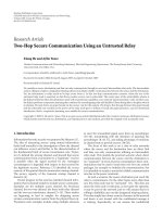
We also approximated a camera network using 15 real images
of a building captured by a single camera from different loca-
tions (Figure 5). The corresponding vision graph is shown in
Figure 6 and was obtained by the automatic algorithm also
described in this special issue [25].Theimagesweretaken
with a Canon G5 dig ital camera in autofocus mode (so that
the focal length for each camera is different and unknown).
A calibration grid was used beforehand to verify that for this

camera, the skew was negligible, the principal point was at
the center of the image plane, the pixels were square, and
there was virtually no lens distortion. Hence the assumed
pinhole projection model with a diagonal K matrix is jus-
tified in this case.
As in the previous experiment, we obtained the dis-
tributed initial calibration estimate using the procedure de-
scribed in Section 3. We analyzed the performance of the
algorithm by measuring the consistency of the camera pa-
rameters before and after belief propagation. Ta ble 3 sum-
marizes the result. Since the ground-truth dimensions of the
scene are unknown, the units of the camera center standard
deviation are arbitrary. The performance is best judged by
the improvement factor, which is quite significant for the
camera centers (a factor of almost 6), which would be impor-
tant for good performance on higher-level vision and sensor
networking algorithms in the real network.
Figure 7 shows the multiple estimates of a subset of the
cameras (aligned to the same coordinate frame) both before
and after the BP algorithm. Before belief propagation, the es-
timates of each camera’s position are somewhat spread out
and there are several outliers (e.g., one estimate of camera
13 is far from the other two, and very close to the corner
of the building). After belief propagation, the improvement
in consistency is apparent; multiple estimates of the same
camera are tightly clustered together. The overall accuracy of
8 EURASIP Journal on Advances in Signal Processing
1 2 3 4 5
6 7 8 9 10
11 12 13 14 15

Figure 5: The 15-image data set used for the experiment on real images.
1
2
3
4
5
6
7
89
10
11
12
13
14
15
Figure 6: Vision graph corresponding to the image set in Figure 5.
the calibr ation can also be judged by the quality of the re-
constructed 3D building structure; for example, the feature
points on the walls of the building clearly fall into parallel
and perpendicular lines corresponding to the entryway and
corner of the building visible in Figure 5. The 3D structure
points are obtained using back-projection and tr iangulation
of corresponding feature points [28].
7. CONCLUSIONS
We demonstrated the viability of using belief propagation to
obtain the accurate, consistent calibration of a camera net-
work in a fully distributed framework. We took into consid-
eration several unique practical aspects of working with sets
of camera parameters, such as overdetermined parameter-
Table 3: Summary of the calibration consistency. C

sd
is the average
standard deviation of error in camera centers (in arbitrary units).
θ
sd
is the average standard deviation of orientation error between
rotation matrices given by (15). f
sd
is the average standard deviation
of absolute focal length error in pixels.
Network state C
sd
θ
sd
f
sd
(pixels)
Initialization 0.1062 0.7692 126.81
Convergence 0.0184 0.3845 84.22
Improvement factor 5.77 2 1.5
izations, frame alignment, and inconsistent estimates. Our
algorithm is distributed, with computations based only on
local interactions, and hence is scalable. The improvement
in consistency is achieved with only a small loss of accuracy.
In comparison, a centralized bundle adjustment would in-
volve an optimization over a huge number of parameters and
would pose challenges for scalability of the algorithm.
The framework proposed here could also incorporate
other recently proposed algorithms for robust distributed in-
ference, as descr ibed in Section 2. While the forms of the

passed messages might change, we believe that our insights
into the fundamental challenges of dealing with camera net-
works would remain useful. Improved inference schemes
might also have the benefit of allowing asynchronous updates
(since BP as we described it here is implicitly synchronous).
D. Devarajan and R. J. Radke 9
1
1
1
2
2
23
3
3
8
10
13
13
Entryway
Sidewall
(a)
1
2
3
8
10
13
Entryway
Sidewall
(b)

Figure 7: Multiple camera estimates of a subset of cameras (a) be-
fore and (b) after belief propagation. The numbers correspond to
the node numbers in Figures 5 and 6.
In the future, we plan to investigate higher-level dis-
tributed vision applications on camera networks, such as
shape reconstruction and object tracking, which further
demonstrate the importance of using consistently localized
cameras. Finally, we plan to analyze networking aspects of
our algorithm (e.g., effects of channel noise or node failures)
that would be important in a real deployment.
ACKNOWLEDGMENT
This work was supported in part by the US National Foun-
dation, under the award IIS-0237516.
REFERENCES
[1]L.Davis,E.Borovikov,R.Cutler,D.Harwood,andT.Hor-
prasert, “Multi-perspective analysis of human action,” in Pro-
ceedings of the 3rd International Workshop on Cooperative Dis-
tributed Vision, Kyoto, Japan, November 1999.
[2] T. Kanade, P. Rander, and P. J. Narayanan, “Virtualized reality:
constructing virtual worlds from real scenes,” IEEE Multime-
dia, Immersive Telepresence, vol. 4, no. 1, pp. 34–47, 1997.
[3] H. F. Durrant-Whyte and M. Stevens, “Data fusion in decen-
tralized sensing networks,” in Proceedings of the 4th Interna-
tional Conference on Information Fusion, pp. 302–307, Mon-
treal, Canada, August 2001.
[4] R. Smith, M. Self, and P. Cheeseman, “Estimating uncertain
spatial relationships in robotics,” in Autonomous Robot Vehi-
cles, pp. 167–193, Springer, New York, NY, USA, 1990.
[5] S. Grime and H. F. Durrant-Whyte, “Communication in de-
centralized systems,” IFAC Control Engineering Practice, vol. 2,

no. 5, pp. 849–863, 1994.
[6] K.P.Murphy,Y.Weiss,andM.I.Jordan,“Loopybeliefpropa-
gation for approximate inference: an empirical study,” in Pro-
ceedings of Uncertainty in Artificial Intelligence (UAI ’99),pp.
467–475, Stockholm, Sweden, July-August 1999.
[7] J. Pearl, Probablistic Reasoning in Intelligent Systems,Morgan
Kaufmann, San Francisco, Calif, USA, 1988.
[8] W. T. Freeman and E. C. Pasztor, “Learning to estimate scenes
from images,” in Advances in Neural Information Processing
Systems 11,M.S.Kearns,S.A.Solla,andD.A.Cohn,Eds.,
MIT Press, Cambridge, Mass, USA, 1999.
[9]B.J.Frey,Graphical Models for Pattern Classification, Data
Compression and Channel Coding, MIT Press, Cambridge,
Mass, USA, 1998.
[10] R. J. McEliece, D. J. C. MacKay, and J F. Cheng, “Turbo decod-
ing as an instance of Pearl’s “belief propagation” algorithm,”
IEEE Journal on Selected Areas in Communications, vol. 16,
no. 2, pp. 140–152, 1998.
[11] Y. Weiss and W. T. Freeman, “Correctness of belief propaga-
tion in Gaussian g raphical models of arbitrary topology,” in
Advances in Neural Information Processing Systems (NIPS ’99),
vol. 12, Denver, Colo, USA, November-December 1999.
[12] J. S. Yedidia, W. Freeman, and Y. Weiss, “Understanding belief
propagation and its generalizations,” in Exploring Artificial In-
telligence in the New Millennium,G.LakemeyerandB.Nebel,
Eds., chapter 8, pp. 239–236, Morgan Kaufmann, San Mateo,
Calif, USA, 2003.
[13] M. Isard and A. Blake, “CONDENSATION—conditional den-
sity propagation for visual tracking,” International Journal of
Computer Vision, vol. 29, no. 1, pp. 5–28, 1998.

[14] W. T. Freeman, E. C. Pasztor, and O. T. Carmichael, “Learn-
ing low-level vision,” International Journal of Computer Vision,
vol. 40, no. 1, pp. 25–47, 2000.
[15] J. M. Coughlan and S. J. Ferreira, “Finding deformable shapes
using loopy belief propagation,” in Proceedings of the 7th Euro-
pean Conference on Computer Vision (ECCV ’02), pp. 453–468,
Springer, London, UK, May-June 2002.
[16]P.F.FelzenszwalbandD.P.Huttenlocher,“Efficient be-
lief propagation for early vision,” in Proceedings of the IEEE
Computer Society Conference on Computer Vision and Pattern
Recognition, vol. 1, pp. 261–268, Washington, DC, USA, June-
July 2004.
[17] E. B. Sudderth, M. I. Mandel, W. T. Freeman, and A. S. Willsky,
“Distributed occlusion reasoning for tracking with nonpara-
metric belief propagation,” in Advances in Neural Information
10 EURASIP Journal on Advances in Signal Processing
Processing Systems,L.K.Saul,Y.Weiss,andL.Bottou,Eds.,
vol. 17, pp. 1369–1376, MIT Press, Cambridge, Mass, USA,
2005.
[18] M.Alanyali,S.Venkatesh,O.Savas,andS.Aeron,“Distributed
Bayesian hypothesis testing in sensor networks,” in Proceed-
ings of the American Control Conference, vol. 6, pp. 5369–5374,
Boston, Mass, USA, June-July 2004.
[19] C. Christopher and P. Avi, “Loopy belief propagation as a ba-
sis for communication in sensor networks,” in Proceedings of
the 19th Annual Conference on Uncertainty in Artificial Intelli-
gence (UAI ’03), pp. 159–166, Morgan Kaufmann, San Fran-
cisco, Calif, USA, August 2003.
[20] M. A. Paskin and C. E. Guestrin, “Robust probabilistic in-
ference in distributed systems,” in Proceedings of the 20th

Conference on Uncertainty in Artificial Intelligence (UAI ’04),
pp. 436–445, AUAI Press, Banff Park Lodge, Banff, Canada,
July 2004.
[21] M. A. Paskin, C. E. Guestrin, and J. McFadden, “A robust ar-
chitecture for inference in sensor networks,” in 4th Interna-
tional Symposium on Information Processing in Sensor Networks
(IPSN ’05), Los Angeles, Calif, USA, April 2005.
[22] F. Dellaert, A. Kipp, and P. Krauthausen, “A multifrontal
QR factorization approach to distributed inference applied to
multirobot localization and mapping,” in Proceedings of the
National Conference on Artificial Intelligence (AAAI ’05), vol. 3,
pp. 1261–1266, Pittsburgh, Pa, USA, July 2005.
[23] S. Funiak, C. Guestrin, M. Paskin, and R. Sukthankar, “Dis-
tributed localization of networked cameras,” in The 5th Inter-
national Conference on Information Processing in Sensor Net-
works (IPSN ’06), Nashville, Tenn, USA, April 2006.
[24] P. Sturm and B. Triggs, “A factorization based algorithm for
multi-image projective structure and motion,” in Proceedings
of the 4th European Conference on Computer Vision (ECCV
’96), pp. 709–720, Cambridge, UK, April 1996.
[25] Z. Cheng, D. Devarajan, and R. J. Radke, “Determining vision
graphs for distributed camera networks using feature digests,”
to appear in EURASIP Journal of Applied Signal Processing,spe-
cial issue on Visual Sensor Networks.
[26] D. Devarajan, R. Radke, and H. Chung, “Distributed metric
calibration of ad-hoc camera networks,” ACM Transactions on
Sensor Networks, vol. 2, no. 3, 2006.
[27] M. Pollefeys, R. Koch, and L. Van Gool, “Self-calibration and
metric reconstruction in spite of varying and unknown inter-
nal camera parameters,” in Proceedings of the 6th IEEE Interna-

tional Conference on Computer Vision (ICCV ’98), pp. 90–95,
Bombay, India, Januar y 1998.
[28] M. Andersson and D. Betsis, “Point reconstruction from noisy
images,” Journal of Mathematical Imaging and Vision, vol. 5,
pp. 77–90, 1995.
[29] M. A. Fischler and R. C. Bolles, “Random sample consensus: a
paradigm for model fitting with applications to image analy-
sis and automated cartography,” Communications of the ACM,
vol. 24, no. 6, pp. 381–395, 1981.
[30] B. Triggs, P. McLauchlan, R. Hartley, and A. Fitzgibbon,
“Bundle adjustment—a modern synthesis,” in Vision Algo-
rithms: Theory and Practice, W. Triggs, A. Zisserman, and R.
Szeliski, Eds., Lecture Notes in Computer Science, pp. 298–
375, Springer, New York, NY, USA, 2000.
[31] J. Besag, “Spatial interaction and the statistical analysis of lat-
tice systems,” Journal of the Royal Statistical Society, Series B,
vol. 36, pp. 192–236, 1974.
[32] J. Hammersley and P. E. Clifford, “Markov fields on finite
graphs and lattices,” preprint, 1971.
[33] F. R. Kschischang, B. J. Frey, and H A. Loeliger, “Factor graphs
and the sum-product algorithm,” IEEE Transactions on Infor-
mation Theory, vol. 47, no. 2, pp. 498–519, 2001.
[34] R. Hartley and A. Zisserman, Multiple View Geometry in Com-
puter Vision, Cambridge University Press, Cambridge, UK,
2000.
[35] K. Kanatani and D. D. Morris, “Gauges and gauge transfor-
mations for uncertainty description of geometric structure
with indeterminacy,” IEEE Transactions on Information The-
ory, vol. 47, no. 5, pp. 2017–2028, 2001.
Dhanya Devarajan received her Bachelors

of Engineering (B.E.) degree in electronics
and communications engineering from the
Thiagarajar College of Engineering, Madu-
rai, India, in 1999, and her M.Sc. Eng. de-
gree in electrical engineering from the In-
dian Institute of Science, Bangalore, India,
in 2002. She is currently working towards
her Ph.D. degree in the Department of Elec-
trical, Computer, and Systems Engineering
at Rensselaer Polytechnic Institute, Troy, NY, USA. Her research in-
terests include computer vision, pattern recognition, and statistical
learning in visual sensor networks.
Richard J. Radke received the B.A. degree in
mathematics and the B.A. and M.A. degrees
in computational and applied mathematics,
all from Rice University, Houston, Tex, in
1996, and the Ph.D. degree from the Elec-
trical Engineering Department, Princeton
University, Princeton, NJ, in 2001. For his
Ph.D. research, he investigated several esti-
mation problems in digital video, includ-
ing the synthesis of photorealistic “virtual
video,” in collaboration with IBM’s Tokyo Research Laboratory.
HehasalsoworkedattheMathworks,Inc.,Natick,Mass,devel-
oping numerical linear algebra and signal processing routines. He
joined the faculty of the Department of Electrical, Computer, and
Systems Engineering, Rensselaer Polytechnic Institute, Troy, NY, in
August 2001, where he is also associated with the National Science
Foundation Engineering Research Center for Subsurface Sensing
and Imaging Systems ( CenSSIS). His current research interests in-

clude deformable registration and segmentation of three- and four-
dimensional biomedical volumes, machine learning for radiother-
apy applications, distributed computer vision problems on large
camera networks, and modeling 3D environments with visual and
range data. He received a National Science Foundation CAREER
Award in 2003, and is a Senior Member of the IEEE.