Báo cáo hóa học: " Research Article Fast Discrete Fourier Transform Computations Using the Reduced Adder Graph Technique" pptx

Hindawi Publishing Corporation
EURASIP Journal on Advances in Signal Processing
Volume 2007, Article ID 67360, 8 pages
doi:10.1155/2007/67360
Research Article
Fast Discrete Fourier Transform Computations Using
the Reduced Adder Graph Technique
Uwe Meyer-B
¨
ase,
1
Hariharan Natarajan,
1
and Andrew G. Dempster
2
1
Department of Electrical and Computer Engineering, Florida State University, 2525 Pottsdamer Street, Tallahassee,
FL 32310-6046, USA
2
School of Surveying and Spatial Information Systems, University of New South Wales, Sydney 2052, Australia
Received 28 February 2006; Revised 23 November 2006; Accepted 17 December 2006
Recommended by Irene Y. H. Gu
It has recently been shown that the n-dimensional reduced adder graph (RAG-n) technique is beneficial for many DSP applications
such as for FIR and IIR filters, where multipliers can be grouped in multiplier blocks. This paper highlights the importance of DFT
and FFT as DSP objects and also explores how the RAG-n technique can be applied to these algorithms. This RAG-n DFT will
be shown to be of low complexity and possess an attractively regular VLSI data flow when implemented with the Rader DFT
algorithm or the Bluestein chirp-z algorithm. ASIC synthesis data are provided and demonstrate the low complexity and high
speed of the design when compared to other alternatives.
Copyright © 2007 Hindawi Publishing Corporation. All rights reserved.
1. INTRODUCTION
The discrete Fourier transform (DFT) and its fast implemen-

tation, the fast Fourier transform (FFT), have both played a
central role in digital signal processing. DFT and FFT algo-
rithms have been invented (and reinvented) in many varia-
tions. As Heideman et al. [1] have pointed out, we know that
Gauss used an FFT-type algorithm we now call the Cooley-
Tukey FFT.
We will follow the terminology introduced by Burrus [2],
who classified FFT algorithms according to the (multidimen-
sional) index maps of their input a nd output sequences. We
will therefore call all algorithms which do not use a multi-
dimensional index map DFT algorithms, although some of
them, such as the Winograd DFT algorithms, enjoy an essen-
tially reduced computational effort.
In a recent EURASIP paper by Macleod [3], the adder
costs were discussed of rotators used to implement the com-
plex multiplier in fully pipelined FFTs for 13 different meth-
ods, ranging from the direct method and 3-multiplier meth-
ods to the matrix CSE method and CORDIC-based designs.
It was determined that not a single structure gave the best re-
sults for all twiddle factor values. On average the CORDIC-
based method gave the best results for single multiplier costs.
In this paper, we restrict our design to the two most popu-
lar methods (4
× 2+ and 3 × 5+) used in FFT cores [4, 5]by
FPGA vendors.
The literature provides many FFT design examples. We
found implementations with programmable signal proces-
sors and ASICs [6–10]. FFTs have also been developed using
FPGAs for 1D [11, 12] and 2D transforms [13, 14].
This paper deals with the implementation of two alterna-

tives of fast DFTs via a transformation into an FIR filter. The
methods are called a Rader DFT algorithm and a Bluestein
chirp-z transform. We will present latency data (measured in
clock cycles) when the FFT-block is used in a microproces-
sor coprocessor configuration. The design data are compared
with direct matrix multiplier DFT methods and radix-2 and
radix-4 type Cooley-Tukey based FFTs as used by FPGA ven-
dors [5]. The provided area data are measured in equivalent
gates as typical for cell-based ASIC designs.
2. CONSTANT COEFFICIENT MULTIPLICATIONS
DSP algorithms are MAC intensive. Essential savings are pos-
sible if the multiplications are constant and not variable. Sta-
tistically, half the digits will be zero in the two’s complement
coding of a number. As a result, if a constant coefficient is
realized with an array multiplier,
1
on average 50% of the par-
tial products will also be zero. In the case of a canonic signed
1
An array multiplier is usually synthesized by an ASIC tool in a binary
adder tree structure.
2 EURASIP Journal on Advances in Signal Processing
Multiplier
block
, x[1], x[3], x[2], x[6], x[4], x[5]
Permuted input sequence
W
5
7
W

4
7
W
6
7
W
2
7
W
3
7
W
1
7
x[0]
+
z
−1
+
z
−1
+
z
−1
+
z
−1
+
z
−1

+
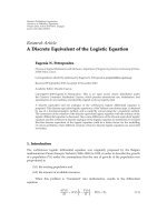
DFT: X[5], X[4], X[6], X[2], X[3], X[1]
Figure 1: Length p = 7 Rader prime factor DFT implementation.
digit (CSD) system, that is, digits with the ternary values
{0, 1, −1}={0, 1, 1}, and no two adjacent nonzero digits,
the density of the nonzero elements becomes 33%. However,
sometimes it can be more efficient to first factor the coef-
ficient into several factors, thus realizing the individual fac-
tors in an optimal CSD sense [15–18]. This multiplier adder
graph (MAG) representation reduces, on average, the imple-
mentation effort to 25% when compared to the number of
product terms used in an array multiplier [3, 19].
In many DSP algorithms, we can achieve additional cost
reduction if we combine several multipliers within a multi-
plier block. The tr ansposed FIR filter show n in Figure 1 is
a typical example for a multiplier block. It has been noted
by Bull and Horrocks [15, 16] that such a multiplier block
can be implemented very efficiently. Later, Dempster and
Macleod [20] introduced a systematic algorithm, which pro-
duces an n-dimensional reduced adder graph (RAG-n)ofa
block multiplier. In general, however, finding the optimal
RAG-n is an NP-hard problem. RAG-n determines when
the design is optimal; for the suboptimal case, heuristics are
used. The full 10-step RAG-n algorithms can be found in
[20].
Another alternative to implementing multiple constant
multiplication is to use the subexpression technique first in-
troduced by Hartley [21]. Here, common patterns in the CSD
coding are identified and successively combined. For random
coefficients, minor improvements were observed compared

with RAG-n. For multiplier blocks with redundancy, RAG-n
generally offered the best per formance [23].
3. FIR FILTER STRUCTURES USED TO
COMPUTE THE DFT
FIR filters are widely studied DSP structures. Their behavior
in terms of quantization error, BIBO stability, and the ability
to build fast-pipelined structures make FIR filters very attrac-
tive. Two algorithms have been used to compute the DFT via
the FIR struc ture. These two are the Rader algorithm, which
requires an I/O data permutation and a cyclic convolution,
and the Bluestein chirp-z algorithm, which uses a complex
I/O multiplication and a linear FIR filter. These two algo-
rithms are briefly reviewed below. Details can be found in
the DSP textbooks [24, 25], as well as in a wide variety of
FFT books [26–30].
The DFT is defined as follows:
X[k]
=
N−1

n=0
x[ n]W
nk
N
k, n ∈ Z
N
, W
N
= e
j2π/N

. (1)
The Rader algorithm [31, 32] used to compute the DFT is
defined only for prime length N.BecauseN
= p is a prime,
we know that there is a primitive element, a generator g, that
generates all elements of n and k in the field
Z
p
, excluding
zero. We substitute n with g
n
mod N and k through g
k
mod
N and get the following index transform:
X

g
k
mod N

− x[0] =
N−2

n=0
x

g
n
mod N


W
g
n+k mod (N−1)
N
(2)
for k
∈{1, 2, 3, , N − 1}. We notice that the right-hand
side of (2) is a cyclic convolution, that is,

x

g
0
mod N

, x

g
1
mod N

, , x

g
N−2
mod N




W
N
, W
g
N
, , W
g
N−2mod(N−1)
N

.
(3)
The DC component must be computed separately as
X[0]
=
N−1

n=0
x[ n]. (4)
Figure 1 shows the Rader algorithm for N
= 7 using the mul-
tiplier block technique.
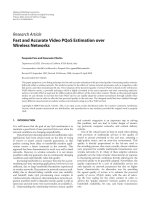
The second algorithm that transforms a DFT into an FIR
filter is the Bluestein chirp-z transform (CZT) algorithm.
Here the DFT exponent nk is a quadratic expanded to
nk
=−
(k − n)
2
2

+
n
2
2
+
k
2
2
. (5)
The DFT therefore becomes
X[k]
= W
k
2
/2
N
N
−1

n=0

x[ n]W
n
2
/2
N

W
−(k−n)
2

/2
N
. (6)
The computation of the DFT is therefore done in three steps:
(1) N multiplications of x[n]withW
n
2
/2
N
;
(2) linear convolution of x[n]W
n
2
/2
N
∗ W
−n
2
/2
N
;
Uwe Meyer-B
¨
ase et al. 3
x[n]
exp(
− jπn
2
/N)
Permultiplication

with chirp signal
Linear
convolution
exp(− jπk
2
/N)
Postmultiplication
with chirp signal
X[k]
Figure 2: The Bluestein chirp-z algorithm.
Table 1: Number of coefficients and costs of Rader multiplier block
implementation for 12-bit plus sign coefficients.
DFT length 7 17 31 61 127 257
C
N
6 16 30 60 126 256
R
N
6 16 30 60 124 253
CSD
21 59 100 201 428 810
MAG
18 51 85 175 360 688
RAG-n
11 23 35 61 124 237
(3) N multiplications with W
k
2
/2
N

.
This algorithm is graphically interpreted in Figure 2.
For a complete transform, we need a length N linear con-
volution and 2N complex multiplications. The advantage,
compared with the Rader algorithms, is that there is no re-
striction to primes in the transform length N.CZTcanbe
defined for every length.
3.1. RAG-n implementation of DFTs
Because the Rader algorithm is restricted to prime lengths,
there is less redundancy in the coefficients compared with
the Bluestein chirp-z DFT algorithms, which can be defined
for any length. Table 1 shows, for the primes next to length
2
n
, the implementation effort of the circular filter in trans-
posed form. The numbers of adders required to implement
the 12-bit filter coefficients are shown for CSD, MAG [17],
and RAG-n [20].
The first row in Tab le 1 shows the cyclic convolution
length N, which is also next to the number of complex co-
efficients C
N
= N − 1, shown in row 2. Row 3 shows the
number R
N
of different real sin/cos coefficient multiplier that
must be implemented. Comparing row 3 and the worst case
with 2(N
−1) real sin/cos coefficients, we see that redundancy
and trivial coefficients reduce the number of nontrivial coef-

ficients by a factor of 2. The last three rows show the costs
(i.e., the number of adders) for a 12-bit multiplier precision
implementation using CSD, MAG, or RAG-n algorithms, re-
spectively. Note the advantage of RAG-n, especially for longer
filters. RAG-n only requires about 1/3 the adder of CSD-type
filters.
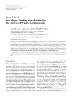
The effort for the CSD, MAG, and RAG-n methods for
all the Rader DFTs up to a length of 257 is graphically inter-
preted in Figure 3.
Narasimha et al. [33] have noticed that in the CZT al-
gorithm many coefficients of the FIR filter part are trivial or
12-bit real coefficients
1200
1000
800
600
400
200
0
Number of adder
0 50 100 150 200 250
DFT length
CSD
MAG
RAG
Figure 3: Effort for a complex multiplier block design in the Rader
algorithm.
Table 2: Number of coefficients and costs of a CZT multiplier block
implemented with 12-bit plus sign coefficients.
N 8 16 32 64 128 256

C
N
47122344 87
R
N
23 61122 43
CSD
6 10 19 38 70 148
MAG
69173462129
RAG-n
57111924 44
identical. For instance, the length-8 CZT has an FIR filter of
length 15, C(n)
= e
j2π((n
2
/2mod8)/8)
, n = 1, 2, , 15, but there
are only four different complex coefficients. These four coef-
ficients are 1, j,and
±e
jπ/8
, that is, we have only two nontriv-
ial real coefficients to implement in the length-8 CZT.
In general, power-of-two lengths are popular building
blocks for Cooley-Tukey FFTs, so we use N
= 2
n
in Tabl e 2

for a comparison.
The comparison of Table 2 with the Rader data shown in
Tabl e 1 shows the advantages of the CZT implementation.
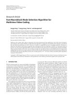
The effort for the CSD, MAG, and RAG-n methods for
the CZT DFT up to a length of 256 is graphically interpreted
in Figure 4. Note that the DFTs with a maximum transform
length are connected through an extra solid line. Due to co-
efficient redundancy explored in the CZT design, we see that
some longer transform lengths may have a lower implemen-
tation effort than some shorter transforms. For this reason,
we might try to use the longer transform whenever possible.
3.2. Complex RAG-n DFT implementations
Thus far we have implemented a DFT of a real input sequ-
ence; the complex twiddle factor multiplication W
nk
n
is im-
plemented with two real multiplications. For complex in-
put DFTs, we have two choices for how to implement the
complex multiplication. We might use a straightforward
approach with 4 real multiplications and 2 real additions:
(a + jb)(c + js)
= a × c − b × s + j(a × s + b × c). (7)
4 EURASIP Journal on Advances in Signal Processing
12-bit real coefficients
200
150
100
50
0

Number of adder
0 50 100 150 200 250
DFT length
CSD
MAG
RAG
Figure 4: Effort for a real coefficient multiplier block design in the
Bluestein chirp-z algorithm. The solid line shows the maximum
transform length for a specific cost value.
Or, we might use a different factorization such as
s[1]
= a − b, s[2] = c − s, s[3] = c + s,
m[1]
= s[1]s, m[2] = s[2]a, m[3] = s[3]b,
s[4]
= m[1] + m[2], s[5] = m[1] + m[3],
(a + jb)(c + js)
= s[4] + js[5],
(8)
which uses 3 real multiplications and 5 real additions,
2
as
shown in Figure 5.
Figure 7 shows that for a transform length of up to 257,
the algorithm with 4
× 2+ is superior (for both Rader and
CZT) when compared with the 3
×5+ algorithms. This is due
to the fact that with the 4
× 2+ algorithms for a filter with N

complex c oefficients, two multiplier blocks with size 2N are
designed, while for the 3
×5+ algorithms three real multiplier
block filters with block size N must be used. To have cleaner
results, we do not show the implementation effort for all CZT
lengths; only the maximum transform lengths for the same
implementation effort are shown.
The overall adder budget now consists of three parts: (a)
the multiplier-block adders, used for CSD, MAG, or RAG
coding; (b) the two output adders required to compute the
complex multiplier outputs; and (c) the 2 structural adders
used for each tap. Because CZT uses only a few different co-
efficients, the required number for (b) is much smaller than
for the Rader transform. However, the filter structure for the
CZT is about twice as long when compared with the Rader
transform. Ta ble 3 shows a comparison for the overall adder
budget required for a CZT of length 64 and a Rader trans-
form of length 61. Again, the direct comparison of Rader and
CZT shows a reduced effort for CZT.
2
Note that in the 3∗×5+ block multiplier architecture, the sum s[2] = c−s
and s[3]
= c + s is precomputed and is therefore sometimes called a 3 ×3+
algorithm.
(a + jb) × (c + js) = R + jI
×
×
×
×
+

+
−
R
I
(a)
(a + jb) × (c + js) = R + jI
+
× +
−
R
+
×
−
+ × +
I
(b)
Figure 5: The two complex multiplier versions (a) 4×2+, (b) 3×5+.
CPU
DFT/FFT
co-processor
Data x, X Program
Figure 6: Co-processor configuration of FFT core.
3.3. Alternative DFT implementations and
synthesis data
In a typical OFDM or DVB configuration [34], the FFT core
is used as a coprocessor to speed up the host processor per-
formance as shown in Figure 6. The computation of the DFT
as coprocessor then has three stages.
(a) The serial data transfer to the coprocessor.
(b) The computation of the DFT, until the first output

value is available.
(c) The data transfer back to the host processor.
While (a) + (c) are usually constants, the latency of the DFT
(b) is a critical design parameter. Table 4 summarizes the
equivalent gate count and the latency of different algorithms.
Uwe Meyer-B
¨
ase et al. 5
12-bit complex coefficients
600
500
400
300
200
100
0
Number of adder
0 50 100 150 200 250
DFT length
3
× 5+ Rader
4
× 2+ Rader
3
× 5+ CZT
4
× 2+ CZT
Figure 7: Comparison of complex multiplier block effort for the
Rader and CZT algorithm.
Table 3: Total required adders for complex DFTs.

CZT-64 points Rader-61 points
CSD MAG RAG CSD MAG RAG
Mul. block 76 68 38 402 350 120
Cmul
22 22 22 120 120 120
Structural
252 252 252 124 124 124
Total 350 342 312 646 594 366
The gate count is measured as equivalent gates as used in cell-
based ASIC design. The latency is the number of clock cycles
the FFT core needs until the first output sample is available
(see (b) above).
Alternative DFT implementations of the CZT RAG-n de-
sign include a direct implementation via DFT matrix multi-
plication [22] using subexpression sharing. Here a length 8
DFT ( 8-bit) already requires 74 adders; a 16-point DFT in
16 bits requires 224 adders.
For short length DFTs, the Winograd algorithm seems
to be an attractive alternative as well, because it reduces the
number of multiplications to a minimum. Unfortunately, the
number of structural adders in the Winograd algorithm in-
creases more than is proportional to the length. For instance,
a complex length 8 DFT requires 52 structural adders [32].
Another common approach uses radix-2 or 4 FFT pro-
cessor elements [5, 35]. A fully pipelined Cooley-Tukey FFT
(called Stream I/O by Xilinx) can benefit from MAG coeffi-
cient coding, but each butterfly in 12-bit precision will re-
quire, on average, 12
× 4 × 25% + 2 = 14 adders. A 64-point
FFT therefore requires 32

×6×14 = 2688 adders if MAG cod-
ing is used. If we use the optimum rotator from [3], then the
required adder can be further reduced to 1684 in a radix-2
scheme. A mixed r adix-2/4 algorithm is reported with 1412
Table 4: Size (measured via equivalent number of gates for com-
binational and noncombinational elements) and speed as latency
(measured as clock cycles until first output value are available) for
different DFT lengths sorted by latency.
Method DFT length
4 8 16 32 64
Matrix Size — 26 640 80 640 — —
Mult.
∗ [22] Latency —22——
Winograd
Size 5129 14 137 36 893 — —
Latency 222——
CSD-CZT
Size 10 349 14 192 23 630 41 426 78 061
Latency 4444 4
RAG-CZT
Size 9970 13 728 22 578 39 234 73 171
Latency 4444 4
Xilinx Radix-2 Si ze — — 29 535 30 455 32 255
Min. Resource [5]
Latency — — 45 112 265
Xilinx Radix-4 Si ze — — — — 137 952
Stream I/O [5]
Latency ———— 64
∗
Estimated.

adders in [3]. In Table 3, the same transform is listed with
312 adders for the chirp-z algorithm.
Minimum FFT resources are achieved with a single radix-
2 Cooley-Tukey butterfly processor (called a minimum re-
source design by Xilinx) at the cost of high latency, shown
as the radix-2 entry in Table 4. Faster but more re source
intensive is a column processor that uses a separate butter-
fly processor in each stage, shown as the radix-4 streaming
I/O in Table 4 [5].
Winograd, CSD, and RAG-n CZT circuits have been
synthesized from their VHDL description and optimized
for speed and size with synthesis tools from Synopsys. The
lsi_10k standard-cell library under typical WWCOM oper-
ating conditions has been used. We used two pipeline stages
for the multiplier and two for the RAG in the design.
From the comparison in Table 4, it can be concluded that
the RAG-CZT provides better results in size compared to the
Winograd DFT or the matrix multiplier for more than 16-
point DFTs. Therefore, only CZT implementations were used
for longer DFTs. When compared with a 64-point Cooley-
Tukey FFT processor, only the single butterfly processor gives
a smaller area, while a faster pipelined streaming I/O proces-
sor requires a 64 clock cycle latency and is twice the size of
the RAG-CZT.
By providing a sufficientamountofextrabuffer mem-
ory all of the above algorithms can be modified in such a
way that the pipelined FFT computation is only limited by
the data transfer time from host to FFT core. This is partic-
ularly useful in 2D FFT, when a large number of consecutive
row/column FFTs need to be computed. However, in 1D DFT

the latency, that is, the number of clock cycles will not change
by adding buffer memory until a value is available at the core
for the (waiting) host processor.
6 EURASIP Journal on Advances in Signal Processing
3.4. Alternative MCM arithmetic concepts
Other possible arithmetic modifications that can be used
to implement the multiple constant multiplication (MCM)
block in fast DFTs are the (exclusive) use of carry-save adders
[36], distributed arithmetic [37], common subexpression
sharing (CSE) [21], or the residue number system (RNS)
[38].
It has also been suggested
3
that the MCM problem can be
considered as a more general design of a 2N
× 2matrixmul-
tiply problem. This will then also cover the two cases 4
× 2+
and 3
×5+ discussed in this paper. However, the conventional
RAG-n algorithm used in this study with a single input and
multiple outputs then needs to be modified to include such
a CSE-like input permutation search. The same idea can also
be applied to the 13 different methods discussed by Macleod
[3]. We have also recently seen successful improvements of
the RAG-n heuristic based on the HCUB metric [39] and the
differential RAG [40], which will be especially beneficial for
coefficient bit widths larger than the 12 bits used in this pa-
per.
Some of the above-mentioned MCM arithmetic concepts

may in fact further improve the implementation effort of the
fast DFT algorithms for certain length or bit width and may
be the basis for further studies. The main result of this pa-
per, however, is that due to recent advances in MCM algo-
rithms, Rader and chirp-z have become viable options over
the conventional radix-2 FFT. This contrasts with previously
accepted understanding, as expressed by Burrus and Parks
[28, page 37], who state: “if implemented on digital hard-
ware, the chirp-z transform does not seem advantageous for
calculating the normal DFT.”
3.5. Quantization noise of alternative DFT algorithms
Since fast DFTs and FFTs can be used, for instance, to imple-
ment a fast convolution, it is important to analyze and deter-
mine the required quantization error of the algorithms. To
simplify our discussion let us make the following assump-
tions that are used in textbooks, like [25, 30].
(a) The quantization errors are uncorrelated.
(b) The errors are uniformly distributed random variables
of (B + 1)-bit signed f ractions, such that the variance
becomes 2
−2B
/12.
(c) The complex multiplication with 4 multiplications has
a quantization error of σ
2
= 4 × 2
−2B
/12 = 2
−2B
/3.

(d) The input signal x is random white noise with variance
σ
2
x
= 1/(3N
2
).
With this assumption we can determine the quantization
noise of the DFT since N source contributes to each output
as
E
DFT
= N × σ
2
. (9)
3
The authors are grateful to an anonymous referee for this suggestion.
From (d) we compute the output variance of the DFT/FFT as
E
X
= E



X[k]


2

=

N−1

n=0
E



x[ n]


2



W
nk
N


,
E
X
= Nσ
2
x
=
1
3N
,
(10)

and the noise-to-output ratio becomes
E
DFT
E
X
= 3N
2
σ
2
. (11)
This results in a one-bit loss in the noise-to-signal ratio as the
length doubles. If inside the DFT a double wide accumulator
is used, the noise reduces to
E
DFT2accu
= σ
2
, (12)
which provides the best performance of all algorithms. The
same results occur with the Rader DFT if we use a double-
width accumulator. For the chirp-z DFT, the input and out-
put complex multiplications introduce another 2σ
2
noise,
and the overall output budget becomes
E
CZT
= 3 × σ
2
(13)

assuming that we use a double width accumulator in the FIR
part for the chirp-z DFT. For the FFT, let us have a look
at the popular radix-2 Cooley-Tukey FFT. Here, a double-
length accumulator does not help to reduce the round-off
noise since the output of the butterfly must be stored in the
same (B
−1)-bit memory location. To avoid overflow, we can
scale the input by N, but the quantization error
E
FFTinput
= N × σ
2
(14)
will be essential. Double FFT length results in a loss of 1 bit
in accuracy. A better approach is to scale at each stage by 1/2.
Then each of the N
= 2
n
output nodes is connected to 2
n−s−1
butterflies and therefore to 2
n−s
noise sources. Thus the out-
put mean-square magnitude of the noise is
E
FFT
= σ
2
n
−1


s=0
2
n−s

1
2

2n−2s−2
= 4σ
2

1 − 0.5
n

≈ 4 × σ
2
,
(15)
and the noise-to-signal ratio becomes
E
FFT
E
X
= 12N × σ
2
. (16)
Now we only have a 1/2-bit per stage reduction in the noise-
to-signal ratio, as first shown by Welch [41]. Table 5 summa-
rizes the results for the different methods.

The noise can be further reduced by using a higher radix
in the FFT, more guard bits, or a block floating-point for-
mat, but these methods will usually require more hardware
resources.
Uwe Meyer-B
¨
ase et al. 7
Table 5: Noise in length N = 2
n
DFT and FFT algorithms width
σ
2
= 2
−2B
/3.
Algorithm type
Noise Noise-to-signal
variance ratio
Direct DFT matrix multiply Nσ
2
3N
2
× σ
2
DFT double width accumulator σ
2
3Nσ
2
Rader double width
FIR accumulator

σ
2
3Nσ
2
Chirp-z DFT 3σ
2
9Nσ
2
Radix-2 FFT input scaling (N − 1)σ
2
3N(N − 1)σ
2
Radix-2 FFT
intermediate scaling
4σ
2
(1 − 0.5
n
)12Nσ
2
(1 − 0.5
n
)
4. CONCLUSION
This paper shows that both Rader and Bluestein Chirp-z
DFTs are viable implement paths for DFT or large Radix FFTs
when the multiplier block is implemented with a reduced
adder graph technique. This paper shows that the CZT offers
lower costs than the Rader design due to the larger number
of redundant coefficients in the CZT, which is beneficial to

RAG-n. The DFT hardware effort in an implementation via
RAG-n CZT has only O(N)effort (i.e., not quadratic O(N
2
)
as for the direct DFT method) and provides a DFT with very
short latency, which is attractive when the DFT is used as a
coprocessor. For a 64-point RAG-CZT, 92% of the resources
are used for the linear filter, 7% for the complex I/O multi-
plier, and 1% for coefficient storage.
From a quantization standpoint, both Rader and Blues-
tein Chirp-z DFTs perform better than the Radix-2 Cooley-
Tukey FFT for fixed-point implementations. The Rader algo-
rithm reaches the minimum quantization error of the direct
matrix DFT algorithm.
ACKNOWLEDGMENTS
The authors would like to thank Xilinx and Synopsys (FSU
ID 10806) for their support under the university program.
Thanks also to the anonymous reviewers for their helpful
suggestions for improving this paper.
REFERENCES
[1] M. T. Heideman, D. H. Johnson, and C. S. Burrus, “Gauss and
the history of the fast Fourier transform,” IEEE Acoustic Speech
& Signal Processing Magazine, vol. 1, no. 4, pp. 14–21, 1984.
[2] C. S. Burrus, “Index mappings for multidimensional formula-
tion of the DFT and convolution,” IEEE Transactions on Acous-
tics, Speech, and Signal Processing, vol. 25, no. 3, pp. 239–242,
1977.
[3] M. D. Macleod, “Multiplierless implementation of rotators
and FFTs,” EURASIP Journal on Applied Signal Processing,
vol. 2005, no. 17, pp. 2903–2910, 2005.

[4] Altera Corporation, FFT: MegaCore Function User Guide,Ver.
2.1.3, 2004.
[5] Xilinx Corporation, “Fast Fourier Transform,” LogiCore v3.1,
November 2004.
[6] B. Baas, “SPIFFEE: an energy-efficient single-chip 1024-
point FFT processor,” 1998, />∼bbaas/
fftinfo.html.
[7] G. Sunada, J. Jin, M. Berzins, and T. Chen, “COBRA: an 1.2
million transistor expandable column FFT chip,” in Proceed-
ings of IEEE International Conference on Computer Design:
VLSI in Computers and Processors (ICCD ’94), pp. 546–550,
Cambridge, Mass, USA, October 1994.
[8] Texas Memory Systems, “TM-66 sw ifft chip,” 1996, http://
www.texmemsys.com.
[9] SHARP Microeletronics, “Bdsp9124 digital signal processor,”
1997, terflydsp.com.
[10] P. Lavoie, “A high-speed CMOS implementation of the Wino-
grad Fourier transform algorithm,” IEEE Transactions on Sig-
nal Processing, vol. 44, no. 8, pp. 2121–2126, 1996.
[11] G. Panneerselvam, P. Graumann, and L. Turner, “Implementa-
tion of fast Fourier tr ansforms and discrete cosine transforms
in FPGAs,” in Proceedings of the 5th International Workshop on
Field-Programmable Logic and Applications (FPL ’95), vol. 975
of Lecture Notes in Computer Science, pp. 272–281, Oxford,
UK, August-September 1995.
[12] G. Goslin, “Using Xilinx FPGAs to desig n custom digital signal
processing devices,” in Proceedings of the DSPX, pp. 565–604,
January 1995.
[13] N. Shirazi, P. M. Athanas, and A. L. Abbott, “Implementa-
tion of a 2-D fast Fourier transform on an FPGA-based cus-

tom computing machine,” in Proceedings of the 5th Interna-
tional Workshop on Field-Programmable Logic and Applications
(FPL ’95), vol. 975 of Lecture Notes in Computer Science,pp.
282–292, Oxford, UK, August-September 1995.
[14] C. Dick, “Computing 2-D DFTs using FPGAs,” in Proceedings
of the 6th International Workshop on Field-Programmable Logic,
Smart Applications, New Paradigms and Compilers (FPL ’96),
vol. 1142 of Lecture Notes in Computer Science, pp. 96–105,
Darmstadt, Germany, September 1996.
[15] D. R. Bull and D. H. Horrocks, “Reduced-complexity digital
filtering structures using primitive operations,” Electronics Let-
ters, vol. 23, no. 15, pp. 769–771, 1987.
[16] D. R. Bull and D. H. Horrocks, “Primitive operator digital fil-
ters,” IEE Proceedings G: Circuits, Devices and Systems, vol. 138,
no. 3, pp. 401–412, 1991.
[17] A. G. Dempster and M. D. Macleod, “Constant integer mul-
tiplication using minimum adders,” IEE Proceedings: Circuits,
Dev ices and Systems, vol. 141, no. 5, pp. 407–413, 1994.
[18] A. G. Dempster and M. D. Macleod, “Comments on “Mini-
mum number of a dders for implementing a multiplier and its
application to the design of multiplierless digital filters”,” IEEE
Transactions on Circuits and Systems II: Analog and Digital Sig-
nal Processing, vol. 45, no. 2, pp. 242–243, 1998.
[19] O. Gustafsson, A. G. Dempster, and L. Wanhammar, “Ex-
tended results for minimum-adder constant integer multipli-
ers,” in Proceedings of IEEE International Symposium on Cir-
cuits and Systems (ISCAS ’02), vol. 1, pp. 73–76, Phoenix, Ariz,
USA, May 2002.
[20] A. G. Dempster and M . D. Macleod, “Use of minimum-adder
multiplier blocks in FIR digital filters,” IEEE Transactions on

Circuits and Systems II: Analog and Digital Signal Processing,
vol. 42, no. 9, pp. 569–577, 1995.
[21] R. T. Hartley, “Subexpression sharing in filters using canonic
signed digit multipliers,” IEEE Transactions on Circuits and
Systems II: Analog and Digital Signal Processing, vol. 43, no. 10,
pp. 677–688, 1996.
8 EURASIP Journal on Advances in Signal Processing
[22] M. D. Macleod and A. G. Dempster, “Common subexpression
elimination algorithm for low-cost multiplierless implementa-
tion of matrix multipliers,” Electronics Letters, vol. 40, no. 11,
pp. 651–652, 2004.
[23] M. D. Macleod and A. G. Dempster, “Multiplierless FIR fil-
ter design algorithms,” IEEE Signal Processing Letters, vol. 12,
no. 3, pp. 186–189, 2005.
[24] S. D. Stearns and D. R. Hush, Digital Signal Analysis, Prentice-
Hall, Englewood Cliffs, NJ, USA, 1990.
[25] A. V. Oppenheim and R. W. Schafer, Discrete-Time Signal Pro-
cessing, Prentice-Hall, Englewood Cliffs, NJ, USA, 1992.
[26] E. Brigham, FFT, Oldenbourg, M
¨
unchen, Germany, 3rd edi-
tion, 1987.
[27] R. Ramirez, The FFT: Fundamentals and Concepts, Prentice-
Hall, Englewood Cliffs, NJ, USA, 1985.
[28] C. Burrus and T. Parks, DFT/FFT and Convolution Algorithms,
John Wiley & Sons, New York, NY, USA, 1985.
[29] D. Elliott and K. Rao, Fast Transforms Algorithms, Analyses, Ap-
plications, Academic Press, New York, NY, USA, 1982.
[30] H. Nussbaumer, Fast Fourier Transform and Convolution Algo-
rithms, Springer, Heidelberg, Germany, 1990.

[31] C. Rader, “Discrete Fourier transform when the number of
data samples is prime,” Proceedings of the IEEE, vol. 56, no. 6,
pp. 1107–1108, 1968.
[32] J. McClellan and C. Rader, Number Theory in Digital Signal
Processing, Prentice-Hall, Englewood Cliffs, NJ, USA, 1979.
[33] M. Narasimha, K. Shenoi, and A. Peterson, “Quadratic resi-
dues: application to chirp filters and discrete Fourier trans-
forms,” in Proceedings of IEEE International Conference on
Acoustics, Speech, and Signal Processing (ICASSP ’76), vol. 1,
pp. 376–378, Philadelphia, Pa, USA, April 1976.
[34] U. Meyer-B
¨
ase, D. Sunkara, E. Castillo, and A. Garcia, “Cus-
tom instruction set NIOS-based OFDM processor for FP-
GAs,” in Wireless Sensing and Processing, vol. 6248 of Pro ceed-
ings of SPIE, Kissimmee, Fla, USA, April 2006, article number
62480O.
[35] S. F. Gorman and J. M. Wills, “Partial column FFT pipelines,”
IEEE Transactions on Circuits and Systems II: Analog and Digi-
tal Signal Processing, vol. 42, no. 6, pp. 414–423, 1995.
[36] O. Gustafsson, A. G. Dempster, and L. Wanhammar, “Multi-
plier blocks using carry-save adders,” in Proceedings of IEEE
International Symposium on Circuits and Systems (ISCAS ’04),
vol. 2, pp. 473–476, Vancouver, BC, Canada, May 2004.
[37] S. A. White, “Applications of distributed arithmetic to digi-
tal signal processing: a tutorial review,” IEEE Transactions on
Acoustics, Speech and Signal Processing Magazine, vol. 6, no. 3,
pp. 4–19, 1989.
[38] M. Soderstrand, W. Jenkins, G. Jullien, and F. Taylor, Residue
Number System Arithmetic: Modern Applications in Digital Sig-

nal Processing, IEEE Press Reprint Series, IEEE Press, New
York, NY, USA, 1986.
[39] Y. Voronenko and M. P
¨
uschel, “Multiplierless multiple con-
stant multiplication,” to appear in ACM Transactions on Algo-
rithms.
[40] O. Gustafsson, “A difference based adder graph heuristic for
multiple constant multiplication problems,” in Proceedings
Proceedings of IEEE International Symposium on Circuits and
Systems (ISCAS ’07), New Orleans, La, USA, May 2007, sub-
mitted.
[41] P. Welch, “A fixed-point fast Fourier transform error analysis,”
IEEE Transactions on Audio and Electroacoustics, vol. 17, no. 2,
pp. 151–157, 1969.
Uwe Meyer-B
¨
ase received his B.S.E.E.,
M.S.E.E., and Ph.D. “Summa cum Laude”
degrees from the Darmstadt University of
Technology in 1987, 1989, and 1995, respec-
tively. In 1994 and 1995, he hold a Postdoc-
toral position in the “Institute of Brain Re-
search” in Magdeburg. In 1996 and 1997, he
was a Visiting Professor at the University of
Florida. From 1998 to 2000, he was a Re-
search Scientist for ASIC Technologies for
The Athena Group, Inc., where he was responsible for develop-
ment of high-performance architectures for digital signal process-
ing. He is now a Professor in the Electrical and Computer Engi-

neering Department at Florida State University. During his gradu-
ate studies, he worked part time for TEMIC, Siemens, Bosch, and
Blaupunkt. He holds 3 patents, has superv ised more than 60 mas-
ter thesis projects in the DSP/FPGA area, and gave four lectures at
the University of Darmstadt in the DSP/FPGA area. In 2003, he was
awarded the “Habilitation” (venia legendi) by the Darmstadt Uni-
versity of Technology a requirement for attaining tenured Full Pro-
fessor status in Germany. He received in 1997 the Max-Kade Award
in Neuroengineering and the Humboldt Research Award in 2005.
He is an IEEE, BME, SP, and C&S Society Member.
Hariharan Natarajan was born on 11th
February 1980, in Chennai, India. After fin-
ishing high school in Hyderabad, India, he
graduated from Madras University with B.S.
degree in instrumentation and control en-
gineering. He started his Masters of Science
programme at Florida State University in
fall 2001 and graduated in Summer 2004.
His area of specialization is digital electron-
ics and ASIC design.
Andrew G. Dempster is Director of Re-
search in the School of Surveying and Spa-
tial Information Systems at the Univer-
sity of New South Wales, Sydney, Australia.
He holds B.E. and M.Eng.Sc. degrees from
UNSW and a Ph.D. from the University of
Cambridge. He worked for several years in
telecommunications and satellite systems,
leading the development of the first GPS re-
ceiver designed in Australia. For nine years,

he held academic positions at the University of Westminster in
London and has been at UNSW since 2004. His research inter-
ests are design of satellite navigation receiver systems, new posi-
tioning technologies, arithmetic circuits, and morphological image
processing.