Báo cáo hóa học: " Research Article Linear Motion Blur Parameter Estimation in Noisy Images Using Fuzzy Sets and Power Spectrum" pptx

Hindawi Publishing Corporation
EURASIP Journal on Advances in Signal Processing
Volume 2007, Article ID 68985, 8 pages
doi:10.1155/2007/68985
Research Article
Linear Motion Blur Parameter Estimation in Noisy Images
Using Fuzzy Sets and Power Spectrum
Mohsen Ebrahimi Moghaddam and Mansour Jamzad
Department of Computer Engineering, Sharif University of Technology, 11365-8639 Tehran, Iran
Received 17 July 2005; Revised 11 March 2006; Accepted 15 March 2006
Recommended by Rafael Molina
Motion blur is one of the most common causes of image degradation. Restoration of such images is highly dependent on accurate
estimation of motion blur parameters. To estimate these parameters, many algorithms have been proposed. These algorithms are
different in their performance, time complexity, precision, and robustness in noisy environments. In this paper, we present a novel
algorithm to estimate direction and length of motion blur, using Radon transform and fuzzy set concepts. The most important
advantage of this algorithm is its robustness and precision in noisy images. This method was tested on a wide range of different
types of standard images that were degraded with different directions (between 0
◦
and 180
◦
) and motion lengths (between 10 and
50 pixels). The results showed that the method works highly satisfactory for SNR > 22 dB and supports lower SNR compared with
other algorithms.
Copyright © 2007 Hindawi Publishing Corporation. All rights reserved.
1. INTRODUCTION
The aim of image restoration is to reconstruct or estimate
an uncorrupted image by using the degraded version of the
same image. One of the most common degradation func-
tions is linear motion blur with additive noise. Equation (1)
shows the relationship between the observed image g(x, y)
and its uncorrupted version f (x, y)[1]:

g(x, y)
= f (x, y) ∗ h(x, y)+n(x, y). (1)
In this equation, h is the blurring function (or point
spread function (PSF)), that is, convolved in the original
image and n is the additive noise function. According to
(1), in order to determine the uncorrupted image, we need
to find the blurring function (h)(i.e.,blur identification)
which is a n ill-posed problem. Finding motion blur parame-
ters in none additive noise environments was addressed in
[2–4], where these researchers tried to extend their algo-
rithms to noisy images as well. The authors in [4, 5]have
divided the image into several windows to reduce noise ef-
fects and to extend their methods to support noisy images.
Linear motion blur identification in noisy images was also
addressed using bispectrum in [3, 6]. This method is not
precise enough because theoretically, to remove the noise by
using this method, many windows are required, which in
practice is impossible. The authors in [3, 6] did not specify
the lowest SNR that their method can support. A different
method was presented for noisy images in [2] where authors
used AR (auto regressive) model to present images and have
proved the lowest allowed SNR that their method can sup-
port. In [7], we presented a method based on mathemati-
cal modeling to estimate parameters in noisy images at low
SNRs.
In many other research areas, fuzzy concepts have been
used to improve the application performance and speed. In
the field of image restoration, some researchers have applied
fuzzy concepts as well, however, most of these works are
in blind restoration. For example, authors in [8]presented

a method that incorporated domain knowledge while pre-
serving the flexibility of the scheme. In the most of other
papers, only the noise removal methods were presented. In
[9, 10] a method was presented using fuzzy concepts to re-
move MF (median filter) side effects such as distortion using
an HFF (histogram fuzzy filter). Authors in [11]presented
a PAFF (parametric adaptive fuzzy filter), which works ef-
fectively when the noise ratio is greater than 20%. In [12],
a rule-based method using local characteristics of the signal
was presented which reduced Gaussian noise effect and pre-
served the edges. In [13], a hierarchical fuzzy approach was
used to perform detail sharpening.
To the best of our knowledge, so far the fuzzy concepts
have not been used in blur identification. In this paper,
we present a novel algorithm using fuzzy sets and Radon
2 EURASIP Journal on Advances in Signal Processing
|H(u, v)|
π/2
u
π/2
v
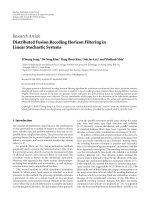
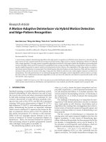
Figure 1: The frequency response of the uniform linear motion blur
(a SINC shape function) with L
= 7.5 pixels, φ = π/4.
transform to find the motion blur parameters in presence or
absence of additive noise. This new method improves our last
works (presented in [1, 7]) by supporting lower SNRs ( i.e., an
improvement between 3–5 dB) and providing more precise
answers.
We have implemented our method using Matlab 7 func-

tions and tested it on 80 randomly selected standard images
of 256
× 256 pixels. The accuracy of our method was e valu-
ated by determining the mean and standard deviation of dif-
ferences between actual and estimated angle/length param-
eters (in the following sections this difference is referred to
as an error). In comparison with other methods listed above,
our method supports lower SNRs. We measured the lowest
allowed SNR in our method experimentally which was about
22 dB in average.
The rest of the paper is organized as follows. In Section 2,
the motion blur parameters are introduced. Section 3 de-
scribes finding parameters in noise free images. The problem
in noisy images and the use of fuzzy sets in motion length es-
timation are addressed in Section 4. Experimental results are
provided in Section 5.InSection 6, we compare our method
with other methods and finally we present the conclusion in
Section 7.
2. MOTION BLUR ATTRIBUTES
The general form of the motion blur function is given as fol-
lows [7]:
h(x, y)
=
⎧
⎪
⎨
⎪
⎩
1
L

,if

x
2
+ y
2
≤
L
2
,
x
y
=−tan(φ),
0, otherwise.
(2)
As seen in (2), motion blur function depends on two
parameters: motion length (L) and motion direction (φ).
Figure 1 shows the frequency response of this function for
L
= 7.5 pixels and φ = π/4.
The frequency response of h is a SINC function. This im-
plies that “if an image is affected only by motion blur and
there is no additive noise, then we can see dominant par-
allel dark lines in its frequency response (Figure 2(b)) that
correspond to very low near-zero values [2, 5, 6, 14, 15].”
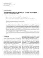
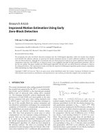
Figure 2 shows the lake image corrupted by motion blur with
(a) (b)
Figure 2: (a) The lake image degraded by linear motion blur using
L
= 20 pixels, φ = 45

◦
, (b) Fourier spectr um of (a).
no additive noise and its Fourier spectrum, in which the par-
allel dark lines are obvious. These parallel dark lines and the
SINC structure in the frequency response of the degrada-
tion function are the most critical data that are used in our
method.
3. MOTION BLUR PARAMETER ESTIMATION IN
NOISE FREE IMAGES
In this sec tion, we propose a solution for cases in which the
image is corrupted by a degradation function without addi-
tive noise (i.e., n(x, y)
= 0).
In the absence of noise, (3) concludes that
G(u, v)
= F(u, v) · H(u, v), (3)
where G(u, v), F(u, v), and H(u, v) are frequency responses
of the observed image, original image, and the degradation
function, respectively. In this case, the motion blur parame-
ters are determined as described in the following subsections.
3.1. Motion direction estimation
To find motion direction, we used the parallel dark lines that
appear in the Fourier spectrum of a degraded image, an ex-
ample of which is shown in Figure 2(b).In[1], we showed
that the motion blur direction (φ) is equal to the angle (θ)
between any of these parallel dark lines and the vertical axis.
Therefore, to find motion direction, it is enough to find the
direction of these parallel dark lines. However, we supposed
I
= log |G(u, v)| is a gray-scale image in spatial domain to

which we can apply any line fitting method to find the di-
rection of a line. Among many line fitting methods that were
applicable, we used Radon transform [16] either in the form
of (4)or(5):
R(ρ, θ)
=

∞
−∞

∞
−∞
g(x, y)δ(ρ − x cos θ − y sin θ)dx dy,
(4)
R(ρ, θ)
=

∞
−∞
g(ρ cos θ − s sinθ, ρ sin θ + s cos θ)ds.
(5)
M. E. Moghaddam and M. Jamzad 3
The advantage of Radon transfor m to other line fitting
algorithms, such as Hough transform and robust regression
[17], is that one does not need to specify candidate points
for the lines. To find direction of these lines, let R be the
Radon transform of an image, then the position of high spots
along the θ axis of R shows the direction [16]. Figure 4 shows
the result of applying Radon transform to the log of Fourier
transform of a n image which was corrupted by a linear mo-

tion blur (direction 45
◦
) with no additive noise. To find the
high spots, we can use any peak detection algorithm like Cep-
strum analysis.
More details of using Radon transform for finding mo-
tion direction are given in our previous work [7].
3.2. Motion length estimation
After finding motion direction, we rotated the coordinate
system of log
|G(u, v)|, rather than rotating the observed im-
age, to align it with motion direction. Rotating the coordi-
nate system solves the problems that occur in image rotation
such as interpolation and out of range pixels. Because of the
rotation effect, some parts of Fourier spectrum will appear
in areas out of the coordinate system support, as a result the
same number of valid data will not be available in a ll columns
in the new coordinate system. Most of valid data is located
in the column passing through frequency center. The pre-
sented algorithm is based on the central peaks and valleys in
the Fourier spectrum, therefore this rotation has no effect on
precision and robustness of the algorithm.
In this case, the uniform motion blur e quation is one-
dimensional like (6)[18]:
h(i)
=
⎧
⎪
⎨
⎪

⎩
1
L
if
−
L
2
≤ i ≤
L
2
,
0 otherwise.
(6)
The continuous Fourier transform of h, which is a SINC
function is shown in (7)[19]:
H
c
(u) =
2Sin(uπL/2)
uπL
. (7)
The discrete version of H in horizontal direction is shown in
(8)[2, 19]:
H(u)
=
Sin(Luπ/N)
L Sin(uπ/N)
,0
≤ u ≤ N − 1, (8)
where N is the image size. To find L we tried to solve the

equation H(u)
= 0, (i.e., finding zero values of a SINC func-
tion). Solving this equation leads to solv ing (9):
Sin

Luπ
N

=
0, (9)
u
=
kπ
LW
such that W
=
π
N
, k>0. (10)
If u
0
and u
1
are two successive zero points such that
H(u
0
) = H(u
1
) = 0, then
u

1
− u
0
=
N
L
(11)
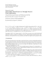
(a) (b)
(c) (d)
Figure 3: (a) A motion blurred image with L = 10 pixels, φ = 45
◦
,
(b) Fourier spectrum of (a), (c) motion blurred image with L
= 30
pixels, φ
= 45
◦
, (d) Fourier spectrum of (c). The sizes of (a) and (c)
are 256
× 256 pixels.
0
45
90
135
180
N
Peak corresponding with line direction
Figure 4: The result of applying Radon transform to the log of
Fourier transform of an image that was degraded using linear mo-
tion blur with direction 45

◦
and no additive noise.
which results in
L
=
N
d
, (12)
where d is the distance between two successive dark lines in
log(
|G(u, v)|).
Figures 3(b) and 3(d) show visualizations of log(
|G(u, v)|)
for two motion blurred sample images. To find d and use it
to calculate L using (12), we should find u such that G(u)
is zero or near zero. Those points for which G(u)isnear
4 EURASIP Journal on Advances in Signal Processing
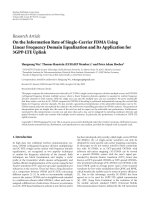
(a) (b)
Figure 5: (a) The image (256×256) of Barbara which is degraded by
motion blur with parameters L
= 30 pixels, φ = 45
◦
and Gaussian
additive noise with zero mean and variance
= 0.04 (SNR = 30 dB).
(b) its Fourier spectr um.
zero are categorized into t wo groups. The first group corre-
sponds to the straight dark lines that are created by motion
blur (H(u)
= 0) and the second group is created by actual

pixel values (F(u)
= 0). To calculate d, we should use the first
group of u. To do this robustly, we used fuzzy set as described
in Section 4.2.
4. MOTION BLUR PARAMETER ESTIMATION IN
NOISY IMAGES
When noise, usually with a Gaussian distribution, is added
to a degraded image, the parallel dark lines in frequency re-
sponse of degraded image become weak and some of them
disappear. If noise variance increases, then more such dark
lines disappear. Figure 5(a) shows Barbara image degraded
by motion blur and additive noise, Figure 5(b) shows the fre-
quency response of Figure 5(a). To overcome the noise effect,
in the following sections we propose a novel, simple, and ro-
bust algorithm based on Radon transform and fuzzy sets to
estimate motion direction and length, respectively.
4.1. Motion direction estimation in noisy images
The concepts we have used here is similar to the one used
for noiseless images. Looking at Figure 5(b) we can see a
white bound around the image center. This white bound is
generated by the SINC structure of frequency response of
motion blur function shown in Figure 1. The direction of
white bound exactly matches with the direction of disap-
peared dark lines, so it also corresponds to the direction of
motion blur. Therefore, to find motion blur direction, it is
enough to find the direction of this white bound, consisting
of several parallel white lines. Using Radon transform, we can
find the direction (θ) of these white lines [7].
4.2. Motion length estimation in noisy images
using fuzzy sets

In presence of noise, the parallel dark lines in frequency re-
sponse of a degr aded image become weak and some of them
disappear. In low SNRs, these dark lines disappear com-
pletely. Equation (13) shows frequency domain version of (1)
0
0.2
0.4
0.6
0.8
1
20 50 100 150 200 230 250
Figure 6: The Z-structure of membership function introduced by
(15) when a
= 20 and c = 230.
in the presence of noise. Here W(u, v)hasdifferent parame-
ters in Gaussian distribution compared to w(x, y):
G(u, v)
= H(u, v) · F(u, v)+W(u, v). (13)
Since noise is a random parameter, its effect on pixels of
a dark line is different. The question is which pixels belong
to the disappeared dark lines. In log(
|G(u, v)|), darker pixels
are better candidates to be a part of a dark line than others.
Which pixels are dark pixels? And can we certainly claim that
the other pixels are not part of a dark line? Because of noise
effects, we cannot answer these questions with certainty. This
uncertainty leads us to use fuzzy concepts to find dar k lines
in frequency response of degraded images. In fact, each pixel
in the frequency response of a degraded image can be a part
of a dark line w i th different possibility, therefore, we define a

fuzzy set for each row of log(
|G(u, v)|) in rotated coordinate
system as follows:
A
i
=

x, μ
n(x)

| x ∈ (1, , N), n(x) = log



G(i, x)



,
(14)
where N is the number of columns in image and i is the row
number. We define the membership function μ
u
as the Z-
function, because the darker pixels are better candidates to
belong to disappeared dark lines while lighter ones are worse
candidates. The z-function models this property using the
following equation:
μ
u

=
⎧
⎪
⎪
⎪
⎪
⎪
⎪
⎪
⎪
⎪
⎪
⎨
⎪
⎪
⎪
⎪
⎪
⎪
⎪
⎪
⎪
⎪
⎩
1, u ≤ a,
1
− 2 ×
(u − a)
(c − a)
2

, a<u≤
(a + c)
2
,
2
×
(u − c)
(c − a)
2
,
(a + c)
2
<u
≤ c,
0, otherwise.
(15)
Figure 6 shows a plot of this function. In (15), a and c are
two constant values that are specified heuristically. The best
values that we found were a
= 20 and c = 230 for a 256 level
gray-scale image. We used the same values of a and c for all
images. The columns of log(
|G(u, v)|) with higher member-
ship values in all sets (A
i
) are the best candidate for the dark
M. E. Moghaddam and M. Jamzad 5
0
0.1
0.2

0.3
0.4
0.5
0.6
0.7
0.8
0.9
1
f (x)
0 50 100 150 200 250
x
Specified valleys
Figure 7: f (x) of an image with no additive noise.
lines. Therefore, we used Zadeh t-norms [20] to find inter-
section of these sets:
B
=

x, μ

x

| μ

x
= t

μ
1x
, , μ

Mx

, x ∈ (1, , N)

.
(16)
In this equation, B is intersection of sets, M is number of
rows in log(
|G(u, v)|), μ
ix
shows the membership value of x
in A
i
,andt is Zadeh t-norm. Now we define f (x), the possi-
bility that column x does not belong to a dark line, as follows:
f (x)
=
⎧
⎨
⎩
1 − μ

x
, x ∈ B,
0, otherwise.
(17)
Figure 7 shows the f (x) that was obtained from a de-
graded image with L = 30 pixels with no additive noise.
Looking carefully at this figure, it is obvious that f (x)has
aSINCstructureandvalleysin f (x) (valleys in the Fourier

spectrum of degradation function) correspond to the dark
lines.
Figure 8 shows f (x) of an image corrupted by linear mo-
tion blur w ith L
= 30 pixels and added Gaussian noise with
σ
2
w
= 1andSNR= 25 dB.
All valleys of f (x) are candidates of dar k line places but
some of them may be false. The best ones are valleys that
correspond to SINC structure in Fourier spectrum of degra-
dation function. These valleys are in two sides of the cen-
tral peak as shown in Figures 7 and 8. By finding these val-
leys using a conventional pitch detection algorithm, their dis-
tance can be calculated. Because of the SINC structure, this
distance is twice the distance between two successive paral-
lel dark lines. Therefore, by using (12)wecanfindmotion
length using the following equation:
L =
2 × N
r
, (18)
where r is the distance between these valleys and N is the
image size. This equation is derived from (12), by setting
d
= r/2, where d is successive lines distance. It is important
to note that the values of f (x) are not the same in differ-
ent images, while f (x) consists of peaks and valleys which
depend on degradation function but not on the image. The

advantage of this algorithm is that it works in low SNR and
its robustness does not depend on L and φ.
0
0.1
0.2
0.3
0.4
0.5
0.6
0.7
0.8
0.9
1
f (x)
0 50 100 150 200 250
x
Specified valleys
Figure 8: f (x) of an image corrupted by linear motion blur with
L
= 30 pixels and additive Gaussian noise (SNR = 25 dB).
5. EXPERIMENTAL RESULTS
We have applied the above algorithms on 80(256
×256) stan-
dard images such as Camera-man, Lena, Barbara, Baboon,
that were degraded by different orientations and lengths of
motion blur (i.e., 0
◦
≤ φ ≤ 180
◦
and 10 ≤ L ≤ 50 pixels).

Then we added Gaussian noise with zero mean and differ-
ent variances (0.01
≤ σ
2
w
≤ 0.61) to these images. To create
a blurred image, three random variables were produced as
follows:
(1) r
L
∈ [0, , 13],
(2) r
φ
∈ [0, , 36],
(3) r
σ
∈ [0, , 12].
Then the blur parameters were calculated using the following
equations:
L
= r
L
× 3 + 10;
φ
= r
φ
× 10;
σ
2
w

= r
σ
× 0.05 + 0.01.
(19)
In each iteration, a degraded image was created using these
parameters. T herefore, regarding intervals defined for r
L
, r
φ
,
r
σ
,and(19), 14 different lengths, 37 different directions and
13 different Gaussian noise variances could be combined to
create a sample set of degraded images. We selected 80 im-
ages from this set to test our algorithm. Then we used our
algorithm to find motion blur parameters of the blurred im-
ages created by the mentioned procedure. Cepstrum analysis,
that is, a standard pitch detection algorithm was used to find
valleys in f (x). Additionally, the properties of SINC struc-
ture of f (x) were used to discard false detected valleys and to
increase the precision of the method. Using this customized
Cepstrum analysis, the valleys around the central peak with
the same distances were accepted. After finding motion blur
parameters, Wiener filter was used to restore the original im-
ages.
Tab le s 1 and 2 show the summary of results. In these ta-
bles, the columns named “angle tolerance” and “length tol-
erance” show the absolute value of errors (the difference be-
tween the actual values of the angle and length and their es-

timated values), respectively. The low values of the mean and
6 EURASIP Journal on Advances in Signal Processing
Table 1: Experimental results of our algorithm on 80 degraded
standard images (256
× 256) with no additive noise.
Cases
Angle tolerance Length tolerance
(degree) (pixels)
Best estimate 00.0
Worst estimate
21.9
Average estimate
0.6 0.9
Standard deviation
0.7 0.4
Table 2: Experimental results of our algorithm on 80 degraded
standard images (256
× 256) with additive noise with zero mean
and 0.01 to 0.6 variance (SNR > 22 dB).
Cases
Angle tolerance Length tolerance
(degree) (pixels)
Best estimate 00.0
Worst estimate
22.5
Average estimate
0.9 0.9
Standard deviation
0.69 0.55
standard deviation of errors show the high precision of our

algorithm. The worst case of the algorithm in estimation of
motion length occurred when L>40 pixels and its best case
happened when 10
≤ L ≤ 26 pixels.
For estimating motion direction, there was no spe cific
range for worst and best cases of the algorithm. These cases
may occur in each direction.
If we define SNR as (20):
SNR
= 10 log
10

σ
2
f
σ
2
w

, (20)
where σ
2
f
denotes image variance and σ
2
w
defines noise vari-
ance, then our algorithm shows a robust behavior at SNR
> 22 dB. Decreasing SNR values increases algorithm estima-
tion error. As an example for a specified image with L

= 18
pixels and SNR
= 15 dB, the motion length estimation error
was about 10 pixels. At SNR
= 20 dB, the estimation error
was about 7 pixels for the same image. Figures 9 and 10 show
noisy degraded images with low SNRs. T heir motion blur pa-
rameters were estimated successfully by our algorithm. Also
we studied the effect of changing the values of parameters
a and c in (15) on the algorithm. The best values for these
parameters were a
= 20 and c = 230, that were calculated
heuristically. Changing the values of a and c in the range of
±5and±10, respectively, did not have significant effect on
algorithm precision. But changing these parameters beyond
these ranges decreases the precision of the algorithm.
6. COMPARISON WITH RELATED METHODS
A comparison with related methods shows that the method
presented in this paper is more robust, has higher precision,
and supports lower SNRs.
Figure 9: Camera picture which was degraded by L = 20 pixels,
φ
= 60
◦
and Gaussian additive noise (SNR = 30 dB). Estimated
values for this image using our algorithm were L
= 21.8 pixels and
φ
= 58.7
◦

.
Figure 10: Baboon picture which was degraded by L = 10 pixels,
φ
= 135
◦
and Gaussian additive noise (SNR = 25 dB). Estimated
values for this image using our algorithm were L
= 8 pixels and
φ
= 136.8
◦
.
In [2], the experimental results were presented briefly
and there was no overall experimental results. Their algo-
rithm was tested only on two degraded images in horizontal
direction using L
= 11 pixels. As authors said, the estimated
length for the first image with SNR
= 40 dB was L = 11.1
pixels which was the same as results for the second image
with SNR
= 30 dB. In addition, the authors presented a re-
stored image with SNR
= 23.3 dB, but they did not present
parameter estimation for this image. The weak point of this
method was that the authors presented results for only two
images. To compare our algorithm with method presented
in [2], we applied our algorithm to similar images with the
same parameters, which resulted in estimation of L
= 11.6

pixels when SNR
= 40 dB and L = 11.8 pixels when SNR
= 30 dB.
Authors in [21] did not discuss additive noise but they
tried to solve the problem in noise free images. T he aver-
age estimation error that they reported in noise free texture
M. E. Moghaddam and M. Jamzad 7
images was 3.0
◦
in direction and 4.1 pixels in length which
were both worst than the ones found in our method under
similar conditions.
In another paper [15] authors presented an estimation
error of 1
◦
–3
◦
in direction and 4–6 pixels in length for noise
free images which are not as good as the ones obtained with
our method.
The authors in [14] did not discuss the precision and
SNR support of their method. It has also a limitation in mo-
tion length where L<15 pixels. Our method has no limita-
tion in motion length in theory. We tested it using L
≤ 50
pixels and the results were satisfactory.
The researchers in [6] did not show the lowest SNR
that their method could support. They reported that their
method worst case estimation error was about 5
◦

in direc-
tion and 2.5 pixels in length. These results were analyzed with
noise variances of 1 and 25.
In addition, the methods given in [3, 22]werevalidfor
SNR as low as 40 dB. The authors did not provide any infor-
mation about the precision of their methods.
The algorithms presented in [4, 5]havenoexhaustiveex-
perimental results.
In our latest work we provided a method that had a pre-
cise estimation of parameters in BSNR > 30 dB (which is
about SNR > 25 dB [7]). Overall, our method supports lower
SNR than other methods and it gives better precision in most
cases.
7. CONCLUSION
In this paper we presented a robust method to estimate the
motion blur parameters, namely, direction and length. Al-
though fuzzy methods are used in many research areas, but
to the best of our knowledge, their usage in blur identifica-
tion have not been reported yet. We used fuzzy set concepts
to find motion length. This is a novel idea in this field. We
showed the robustness of this method for noisy and noiseless
images. To estimate motion direction we used Radon trans-
form. This helped us to overcome the difficulties with Hough
transform and similar methods to find the candidate points
for line fitting.
The main advantage of our algorithm is that it does not
depend on the input image. To evaluate the performance of
our method, we degraded 80 standard images with different
values of motion direction and length. The motion blur pa-
rameters that were estimated by our method were compared

with their initial values for each image. The comparison of
the low value for mean and standard deviation of errors be-
tween the estimated values and the actual ones showed the
high accuracy of our method.
We believe that the performance of motion blur param-
eter estimation algorithms can be improved if the noisy de-
graded images are processed with specific noise removal al-
gorithms which are able to remove noises while preserving
edges. After applying such noise removal methods we can
implement our algorithm for motion blur parameter estima-
tion to obtain better results. In future, we plan to extend our
work to develop such noise removal methods.
ACKNOWLEDGMENT
We highly appreciate Iran Telecommunication Research Cen-
ter for its financial support to this research, that is part of a
Ph.D. thesis.
REFERENCES
[1] M. E. Moghaddam and M. Jamzad, “Finding point spread
function of motion blur using radon transform and modeling
the motion length,” in Proceedings of the 4th IEEE International
Symposium on Signal Processing and Information Technology
(ISSPIT ’04), pp. 314–317, Roma, Italy, December 2004.
[2] Q. Li and Y. Yoshida, “Parameter estimation and restoration
for motion blurred images,” IEICE Transactions on Funda-
mentals of Electronics, Communications and Computer Sciences,
vol. E80-A, no. 8, pp. 1430–1437, 1997.
[3] M. M. Chang, A. M. Tekalp, and A. T. Erdem, “Blur identifi-
cation using the bispectrum,” IEEE Transactions on Acoustics,
Speech, and Signal Processing, vol. 39, no. 10, pp. 2323–2325,
1991.

[4] M. Cannon, “Blind deconvolution of spatially invariant image
blurs with phase,” IEEE Transactions on Acoustics, Speech, and
Signal Processing, vol. 24, no. 1, pp. 58–63, 1976.
[5]R.Bhaskar,J.Hite,andD.E.Pitts,“Aniterativefrequency-
domain technique to reduce image degradation caused by lens
defocus and linear motion blur,” in IEEE Geoscience and Re-
mote Sensing Symposium (IGARSS ’94), vol. 4, pp. 2522–2524,
Pasadena, Calif, USA, August 1994.
[6] C. Mayntz, T. Aach, and D. Kunz, “Blur identification using
a spectral inertia tensor and spectral zeros,” in IEEE Interna-
tional Conference on Image Processing (ICIP ’99), vol. 2, pp.
885–889, Kobe, Japan, October 1999.
[7] M. E. Moghaddam and M. Jamzad, “Blur identification in
noisy images using radon tr ansform and power spectrum
modeling,” in Proceedings of the 12th IEEE International Work-
shop on Systems, Signals and Image Processing (IWSSIP ’05),pp.
347–352, Chalkida, Greece, September 2005.
[8] K H. Yap and L. Guan, “A fuzzy blur algorithm to adaptive
blind image deconvolution,” in Proceedings of the 7th IEEE In-
ternational Conference on Control, Automation, Robotics and
Vision (ICARCV ’02), pp. 34–38, Singapore, Republic of Sin-
gapore, December 2002.
[9] J H. Wang, W J. Liu, and L D. Lin, “Histogram-based fuzzy
filter for image restoration,” IEEE Transactions on Systems,
Man, and Cyberne tics—Part B: Cybernetics, vol. 32, no. 2, pp.
230–238, 2002.
[10] J H. Wang and M D. Yu, “Image restoration by adaptive
fuzzy optimal filter,” in Proceedings of the IEEE International
Conference on Systems, Man and Cybernetics, vol. 1, pp. 845–
848, Vancouver, BC, Canada, October 1995.

[11] J H. Wang and L D. Lin, “Image Restoration using paramet-
ric adaptive fuzzy filter,” in IEEE Conference of the North Amer-
ican Fuzzy Information Processing Society (NAFIPS ’98),Pen-
sacola, Fla, USA, August 1998.
[12] K. Arakawa, “Fuzzy rule-based signal processing and its appli-
cation to image restoration,” IEEE Journal on Selected Areas in
Communications, vol. 12, no. 9, pp. 1495–1502, 1994.
[13] S. Suthaharan, Z. Zhang, and A. Harvey, “FFF: fast fuzzy filter-
ing in image restoration,” in IEEE Region 10 Annual Conference
Speech and Image Technologies for Computing and Telecommu-
nications (TENCON ’97), vol. 1, pp. 9–12, Brisbane, Australia,
December 1997.
8 EURASIP Journal on Advances in Signal Processing
[14] Y. Li and W. Zhu, “Restoration of the image degraded by linear
motion,” in Proceedings of the 10th IEEE International Confer-
ence on Pattern Recognition (ICPR ’90), vol. 2, pp. 147–152,
Atlantic City, NJ, USA, June 1990.
[15] I. M. Rekleitis, “Optical flow recognition from the power spec-
trum of a single blurred image,” in IEEE International Confer-
ence on Image Processing (ICIP ’96), vol. 3, pp. 791–794, Lau-
sanne, Switzerland, September 1996.
[16] P. Toft, The radon transform—theory and implementation,
Ph.D. thesis, Department of Mathematical Modeling, Techni-
cal University of Denmark, Copenhagen, Denmark, June 1996.
[17] R. C. Gonzalez and R. E. Woods, Digital Image Processing,
Prentice Hall, Upper Saddle River, NJ, USA, 2nd edition, 2002.
[18] M. R. Banham and A. K. Katsaggelos, “Digital image restora-
tion,” IEEE Signal Processing Magazine,vol.14,no.2,pp.24–
41, 1997.
[19] A. V. Oppenheim, A. S. Willsky, and S. H. Nawab, Signals and

Systems, Prentice Hall, Upper Saddle River, NJ, USA, 2nd edi-
tion, 1996.
[20] H. J. Zimmermann, Fuzzy Set Theory, Kluwer Academic, Dor-
drecht, The Netherlands, 1996.
[21] I. M. Rekleities, “Steerable filters and cepstral analysis for op-
tical flow calculation from a single blurred image,” in Proceed-
ings of the Vision Interface Conference, pp. 159–166, Toronto,
Ontario, Canada, May 1996.
[22] A. T. Erdem and A. M. Tekalp, “Blur identification based on
bispectrum,” in Proceedings of the European Signal Processing
Conference (EUSIPCO ’90), Barcelona, Spain, September 1990.
Mohsen Ebrahimi Moghaddam received
his M.S. degree in software engineering
from Sharif University of Technology, Tehr-
an, Iran. Currently, he is a Ph.D. Candidate
in the Department of Computer Engineer-
ing, Sharif University. The present work is
the main core of his Ph.D. thesis. His main
research interests are image processing, ma-
chine vision, data structures, and algorithm
design.
Mansour Jamzad has obtained his M.S. de-
gree in computer science from McGill Uni-
versity, Montreal, Canada and his Ph.D. de-
gree in electrical engineering from Waseda
university, Tokyo, Japan. For a period of
two years after graduation he worked as a
Post Doctorate Researcher in the Depart-
ment of Electronics and Communication
Engineering, Waseda University. He became

an Assistant Professor at the Department of
Computer Engineering, Sharif University of Technology, Tehran,
Iran since 1995. He has been teaching digital image processing and
machine vision graduate courses in the last 10 years. He is a Mem-
ber of IEEE and his main research interests are digital image pro-
cessing, machine vision and its applications in industry, robot vi-
sion, and fuzzy systems.