Báo cáo hóa học: " Research Article Underwater Noise Modeling and Direction-Finding Based on Heteroscedastic Time Series" docx

Hindawi Publishing Corporation
EURASIP Journal on Advances in Signal Processing
Volume 2007, Article ID 71528, 10 pages
doi:10.1155/2007/71528
Research Article
Underwater Noise Modeling and Direction-Finding Based on
Heteroscedastic Time Series
Hadi Amiri,
1
Hamidreza Amindavar,
1
and Mahmoud Kamarei
2
1
Department of Electrical Engineering, Amirkabir University of Technology, P.O. Box 15914, Tehran, Iran
2
Department of Electrical and Computer Engineering, University of Tehran, P.O. Box 14395-515, Tehran, Iran
Received 8 November 2005; Revised 29 April 2006; Accepted 29 June 2006
Recommended by Douglas Williams
We propose a new method for practical non-Gaussian and nonstationary underwater noise modeling. This model is very useful
for passive sonar in shallow waters. In this application, measurement of additive noise in natural environment and exhibits shows
that noise can sometimes be significantly non-Gaussian and a time-varying feature especially in the variance. Therefore, signal
processing algorithms such as direction-finding that is optimized for Gaussian noise may degrade significantly in this environment.
Generalized autoregressive conditional heteroscedasticity (GARCH) models are suitable for heavy tailed PDFs and time-varying
variances of stochastic process. We use a more realistic GARCH-based noise model in the maximum-likelihood approach for the
estimation of direction-of-arrivals (DOAs) of impinging sources onto a linear array, and demonstrate using measured noise that
this approach is feasible for the additive noise and direction finding in an underwater environment.
Copyright © 2007 Hindawi Publishing Corporation. All rights reserved.
1. INTRODUCTION
A passive sonar generally employs array processing tech-
niques to resolve problems such as localization of targets

[1, 2]. As a matter of fact, al l the DOA estimation methods
make a crucial assumption for the noise model, that have
a great impact on the performance of DOA estimation. In
the underwater environment, the measurements of additive
noise show that we have non-Gaussian process [3–5]. Nat-
ural and manmade sources such as reverberation and in-
dustrial noise that cause additive noise distribution exhibit
performances far away from the Gaussian model. These fac-
tors are more in coastal and shallow waters. Thus, the algo-
rithms that are optimized for Gaussian distribution will de-
grade in actual experiments. All this mentioned factors give a
stochastic and time-varying nature to the background noise.
Thus, a proper model presentation which could best a nd
simply describe the different features of the realistic back-
ground noise affecting the desired signal is an important
part of a sonar signal processing. In the last decade, after
the seminal works by Engle [6] and Bullerslev [7] there has
been a growing interest in time series modeling of chang-
ing variance or heteroscedasticity. These models have found
a great number of applications in nonstationary time series
such as financial records. Generalized autoregressive condi-
tional heteroscedasticity; for example, GARCH [7], is a time
series modeling technique that uses past variances and the
past variance forecasts to forecast future variances. GARCH
models account for two main characteristics: excess kurtosis;
that is, heavy tailed probability distribution, and the volatility
clustering; that is, large changes tend to follow large changes
and small changes tend to follow small ones, compatible to a
large extent to the additive noises in a natural environment.
We suggested this more realistic dynamic model for additive

noise modeling in array signal processing [ 8]. Now, we offer
this model for the under water noise in passive sonar due to
the facts that the commonly used model for environmental
additive noise exhibits heavier tail than the standard normal
distribution [9], and the conditional heteroscedasticity sug-
gests a time series model in which time-varying var iances a re
presented, that is, a more logical modeling for the dynamic
of the additive noise [7]. Hence, in this paper, we propose
to assume a conditional heteroscedasticity-based t ime series
for underwater noise modeling and that can be used in the
direction-finding approach for passive sonar. This paper is
organized as follows. In Section 2 we present the GARCH
time series. The proposed noise modeling as the underwater
noise and the DOA estimation based on the new noise model
is provided in Section 3 and the simulation results of the pro-
posed method come in Section 4. Some concluding remarks
are provided at the end.
2 EURASIP Journal on Advances in Signal Processing
2. GARCH TIMES SERIES
The exploitation of time series properties has been exten-
sively used in sig nal modeling and parameter estimation.
Forexample,ARMAtimeseriesmodelshavewideapplica-
tions in signal processing such as sonar signal processing and
noise modeling [10, 11]. One of them that has been used in
the past decade, conditional heteroscedasticity time series,
was first introduced by Engle [6] in the context of model-
ing United Kingdom inflation as known autoregressive con-
ditional heteroscedasticity (ARCH). Such models are charac-
terized by being conditionally Gaussian, additionally repre-
sented by a nonconstant and state-dependent variance. How-

ever, in [6, 7, 12, 13], it is shown that a time-varied variance
over time is more useful than a constant one for modeling
non-Gaussian and non-stationary phenomena such as eco-
nomic series. Generalization of ARCH that is proposed in
[7] is called GARCH. Generally speaking, in heteroscedas-
ticity we consider time series with time-varying variance;
the conditional implies a dependence on the observation
of the immediate past, and autoregressive describes a feed-
back mechanism that incorporates past observations into
the present. GARCH then is a mechanism that includes past
variance in the explanation of the future variance. GARCH
models account for heavy tailed PDF as excess kurtosis and
volatility clustering a type of heteroscedasticity. Now, we let
(k) denote a real-valued discrete-time stochastic process,
the GARCH (p, q) process is then given by [7]
(k) ∼ G

0, σ
2
(k)

,
σ
2
(k) = α
2
0
+
q


i=1
α
2
i

2
(k − i)+
p

i=1
β
2
i
σ
2
(k − i),
(1)
where G denotes the Gaussian probability density function
and α
2
0
, α
2
i
,andβ
2
i
are GARCH model coefficients. For ex-
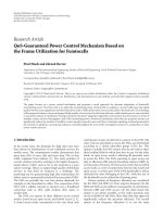
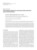
ample, Figure 1 shows some realizations of the GARCH(1, 1)
with different coefficients. The flexibility of GARCH pro-

cess is displayed in this figure, so that some different time
series such as impulsive data can be modeled. This ability
can be obtained due to the complex coefficients structure
of GARCH modeling. The estimation of orders p and q has
an important role in the GARCH modeling of the time se-
ries. Otherwise, because of the importance of the orders in
the computation of coefficients, we should have the proper
consideration for it. In this way, some methods are proposed
such as likelihood ratio tests [14], Akaike information the-
ory criterion (AIC), and Bayesian information criteria (BIC)
[15]. The likelihood ratio tests would be used to determine
supporting the use of a specific GARCH model for a time se-
ries. Using the following order selection methods, AIC, BIC,
and likelihood ratio test, the order that provides the best
model for data fitting is selected.
In this way, we use AIC and BIC information crite-
ria to compare alternative models such as GARCH(1, 1),
GARCH(2, 1) and others. Since information criteria penalize
models with additional parameters, the AIC and BIC model
order selection criteria are based on parsimony [15].
The AIC and BIC statistics are defined as
AIC
=−2L
g
+2N
p
,
BIC
=−2L
g

+ N
p
log(K),
(2)
where L
g
is optimized log-likelihood objective function val-
ues associated with parameter estimates of the GARCH mod-
els to be tested so that the following is obtained:
L
g
=−
K
2
log(2π)
−
1
2
K

k=1
log

σ
2
(k)

−
1
2

K

k=1
n
2
(k)
σ
2
(k)
. (3)
N
p
is the number of GARCH parameters and K is the num-
ber of observations. In the following section, we consider
GARCH-based model for the underwater noise modeling
and DOA estimation in a passive sonar.
3. PROPOSED METHOD
3.1. Underwater noise modeling
Figure 2 shows a general block-diagram of a passive system
such as sonar so that it has as the input process (propagated
source) the underwater channel, the additive noise, and the
observed data in receivers. In this way, we consider the addi-
tive noise comprised of the additive noise and interferences
as follows:
n(k)
= n
P
(k)+n
G
(k), (4)

where n(k) is the received additive noise and interference
in time, n
P
(k) is the interference part, n
G
(k) is the additive
Gaussian noise part, and k stands for the snapshot index.
Due to natural and manmade sources in the underwater en-
vironment, the measurements of noise shows that we have
non-Gaussian process [3–5]. These factors such as reverber-
ation and industrial noise are more in shall ow waters. How-
ever, in practice the noise model is not known because of the
time-varying characteristic of system and non-Gaussian be-
havior of noise source. These are two major factors that can
limit the performance of general methods in the practical ex-
periments. In different applications such as sonar, the time-
varying characteristic is generally due to time-varying nature
of the medium channel, environment, noise, and interfer-
ences [16–19]. For example, underwater acoustic channel is a
time-varying and multipath channel specially in shallow wa-
ter. It varies due to different season, area, and situation of sea
face. The channel variations can be due to the spatial move-
ment of the source and/or changes in the propagation condi-
tions such as sound speed profile. All this mentioned factors
give a stochastic and time-varying nature to the background
noise. Hence, we accept a model in which some kind of
changing variance in time is included. As a result of the above
time-varying events, it can be assumed that the additive
noise has time-varying variance in the receiver. Moreover,
Hadi Amiri et al. 3

10008006004002000
Sample
6
4
2
0
2
4
6
Amplitude
α
2
0
= 1, α
2
1
= 0.1, β
2
1
= 0.4
10008006004002000
Sample
10
5
0
5
10
Amplitude
α
2

0
= 1, α
2
1
= 0.4, β
2
1
= 0.1
10008006004002000
Sample
60
40
20
0
20
40
60
80
Amplitude
α
2
0
= 1, α
2
1
= 0.1, β
2
1
= 0.9
10008006004002000

Sample
40
20
0
20
40
60
Amplitude
α
2
0
= 1, α
2
1
= 0.9, β
2
1
= 0.1
Figure 1: Some realizations of the GARCH(1, 1) with different coefficients.
Source
Channel
Received
data
Noise
Figure 2: System block-diagram.
measurements of the additive noise in related application
such as underwater environment shows that the noise can
sometimes be significantly non-Gaussian and it can be
shown for the widely accepted model of additive noise and
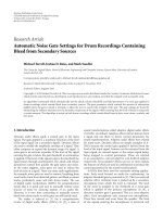
interference excess kurtosis can be observed [5, 9]. For this

purpose, the narrowband Middleton class-A model [20]is
used. This model is a general physical and statistical model
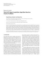
for received additive noise and interference. With (A.5)in
Appendix A, the excess kurtosis is determined as shown in
Figure 3. In this figure the excess kurtosis is shown for the
Middleton class-A model for general values of model pa-
rameters. Thus, the assumed noise model that covers the
properties of additive noise such as time-varying variance
and heavy-tail PDF is more attractive. Under the above as-
sumptions and important features of the GARCH time series
model, we use this model for the additive noise modeling in
10
2
10
3
10
4
10
5
10
6
K
10
0
10
1
10
2
10
3

10
4
Kurtosis (β
2
(n))
A = 10
3
10
2
10
1
1
β
2
= 3
Figure 3: Excess kurtosis in Middleton class-A model.
the underwater acoustics applications such as sonar:
n(k)
∼ GARCH (p, q), (5)
where k
= 1, 2, , K and K is the number of snapshots. At
the start of the modeling technique, we need to the estima-
tion of orders of proposed model, that is, p and q. In this
4 EURASIP Journal on Advances in Signal Processing
0.450.40.350.30.250.20.150.10.050
β
2
1
0
5

10
15
20
25
30
35
40
Kurtosis β
2
()
0.56
0.55
0.54
0.53
0.5
0.45
α
2
1
= 0.4
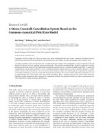
Figure 4: Kurtosis for GARCH(1, 1).
way, we used both AIC and BIC and so the results of our sim-
ulation almost always reached GARCH(1, 1) using recorded
noise. The results of this approach are given in the simulation
section. Therefore,
n(k)
∼ G

0, σ
2

(k)

,(6)
σ
2
(k) = α
2
0
+ α
2
1
n
2
(k − 1) + β
2
1
σ
2
(k − 1). (7)
Generally, the unknown coefficients (α
2
0
, α
2
1
,andβ
2
1
)areesti-
mated using maximum-likelihood method [7].

This model exploits time-varying variance and heavy-tail
PDF for approaching the realistic properties of the additive
noise in practical applications. It is well known that kurto-
sis is an important parameter for analysis of non-Gaussian
random processes. For this purpose, the kur tosis is given by
[7]
β
2
(n) =
E

n
4
(k)


E

n
2
(k)

2
=
3

1 −

α
2

1
+ β
2
1

2

1 −

α
2
1
+ β
2
1

2
− 2α
4
1
. (8)
It can be shown that if (α
2
1
+ β
2
1
) < 1and1− (α
2
1

+ β
2
1
)
2
−
2α
4
1
> 0, then the kurtosis is greater than 3 and GARCH(1, 1)
can conclude heavy-tail PDF. Figure 4 shows the ability of
GARCH modeling for heavy-tail PDF with excess kur tosis.
As it is well known, the assumed noise models can have
an important roles in the signal processing methods such as
parameters estimation. In the following, we propose a new
DOA estimation approach using GARCH noise modeling.
This approach could encompass the DOA estimation not
only in non-Gaussian environment but also it could handel
heavy tailed and nonstationary processes.
3.2. Direction-finding approach
A proper model presentation which could best and simply
describe the different features of the realistic background
noise affecting the desired signal is an important part of
a sonar signal processing, and so the algorithms that are
optimized for Gaussian distribution degrade in actual ex-
periments. The performance of the source localization and
estimation of DOA in passive array applications such as sonar
heavily rely upon the particular array signal processing algo-
rithms used in practice. In these methods, the key assump-
tion is the noise model; that is, additive noise covariance,

that is used in estimation of unknown parameters. Generally,
additive noise is assumed to follow a Gaussian distribution.
However, measurements of acoustic noise and interference
in underwater environment show that the noise can some-
times be significantly non-Gaussian [3–5, 9]. Consequently,
we note that in this model, noise is not uniform across L
sensors, which is a realistic modeling resting on the assump-
tion of non-uniformity [21, 22] and non-stationarity; that is,
time-varying variance. Thus, the assumed noise model that
covers the properties of background noise is more attractive.
Under the above assumption we use the GARCH(1, 1) pro-
cess for the additive noise in direction finding in ar ray signal
processing. Let us assume that a linear array of L omnidi-
rectional hydrophones receives D (D<L) plane wave from
unknown directions of arrivals. The incident plane waves are
assumed to be narrowband with a center frequency. Under
these conditions, the kth snapshot vector of array observa-
tion can be expressed as
x(k)
= A(θ)s(k)+n(k), k = 1, 2, , K,(9)
where s(k) is the D
× 1 vector of the source waveforms, n(k)
is the L
× 1 vector of sensor noise, A(θ) is the L × D steering
matrix
A(θ) 

a

θ

1

, , a

θ
D

, (10)
a(θ
i
) is the direction vectors, θ  {θ
1
, , θ
D
}
T
is the D × 1
vector of the unknown signal DOA, K is the number of snap-
shots, and (
·)
T
stands for the transpose operation. We make
the following assumptions: the signal waveforms are station-
ary; both temporally and spatially, and the signals and noise
are statistically independent of each other. According to the
previous noise modeling section, we propose using the mul-
tivariate GARCH(1, 1) for noise modeling in array sensors
applications such as sonar. Thus, using (6)and(7) the addi-
tive ar ray noise can follow as multivariate GARCH(1, 1) with
zero mean and covariance matrix Q(k), so

n(k)
∼ MG
1,1

n; 0, Q(k)

, (11)
where MG
1,1
stands for the multivariate GARCH(1, 1), and
Q(k)
= diag

σ
2
1
(k), σ
2
2
(k), , σ
2
L
(k)

. (12)
In this approach, the additive noise model at every sensor
is distributed similar to (6)and(7). Same as (9), another
application of GARCH model can be seen in [23] that is
used in the adaptive portfolio management based on max-
imum likelihood in state space method. Consequently (it is

well known) one of the efficient methods in the estimation
of parameters in array signal processing is the ML approach
[11, 24, 25]. For this method, the key assumption is the
noise model; that is, additive noise covariance that is used in
Hadi Amiri et al. 5
the estimation of unknown para meters. In the following, we
exploit the deterministic maximum-likelihood (DML) ap-
proach model so that the signal waveforms are determinis-
tic unknown sequences. Thus, the joint PDF of the observed
array snapshots using GARCH(1, 1) model is expressed as
p
X|ψ
(X)
=
K

k=1
1
det

πQ(ψ, k)

exp

−

x(k) − A(θ)s(k)

H
× Q

−1
(ψ, k)

x(k) − A(θ)s(k)


,
(13)
where
ψ
=

θ
T
, s
T
, g

, (14)
where g is vector of GARCH(1, 1) coefficients,
s
T
=

s
T
(1), , s
T
(K)


(15)
is the vector of the unknown signal. Therefore, by using (12)
and (13) it can be shown that the following holds for log-
likelihood:
L
p
(ψ) =−
K

k=1
L

=1
ln

σ
2

(k)

−
K

k=1


x(k) − A(θ)s(k)

H
× Q

−1
(ψ, k)

x(k) − A(θ)s(k)


.
(16)
L
p
(·) stands for the proposed log-likelihood func tion to
be maximized over the vector of unknown parameters ψ
through ML approach. Therefore, due to complicated nature
of problems, this estimation cannot be found analytically,
and
−L
p
(·) can be minimized through numerical procedures
[1] a nd then unknown parameters are found. In this way, we
use the gradient-based minimization, the Newton approach.
These methods are based on multidimensional searching
and minimization of log-likelihood function onto parame-
ter space and have heavy computational burden. Generally,
we would like to decrease the number of unknown parame-
ters as much as possible, and also select their feasible initial
values of them at the beginning of the process. As a matter
of fact, the initial values of the bounded parameters are one
of the most important factors in the rate of the convergence
and the computational volume of the minimization process.
In the proposed method we have different unknown parame-

ters in the process. The most important is the DOA of sources
so that they are estimated in our approach. Without loss of
generality, we assume that the number of sources is given and
then we use the popular method such as music to have initial
values of DOAs at the beginning of approach. About noise
model parameters, we considered some constraints on their
values such as α
2
1
≥ 0, β
2
1
≥ 0, and (α
2
1
+ β
2
1
) < 1. Contin-
uously, if we do not have real signal waveforms, then, the
known least square error approach is used for initial estima-
tion [1]. For the statistical analysis of proposed method, the
CRB is derived in Appendix B.
Table 1: Order selection.
Approach AIC BIC
GARCH(1, 1) 1.6384e + 004 1.6452e + 004
GARCH(1, 2)
1.6386e + 004 1.6460e + 004
GARCH(2, 1)
1.6386e + 004 1.6459e + 004

GARCH(2, 2)
1.6387e + 004 1.6466e + 004
4. SIMULATION AND RESULTS
In this section, we demonstrate the performance of the pro-
posed approach for modeling of the additive noise in pas-
sive sonar with two major experiments. In the first exper-
iment, we use the recorded noise with one hydrophone in
shallow water. In this scenario, order selection and estima-
tion of PDFs of the real and simulated data are considered.
Using GARCH noise modeling in the DOA estimation of
the underwater targets are examined in the latter experiment
that utilize uniform linear array (ULA). Root-mean-square-
errors (RMSE) of estimated DOA are considered versus SNRs
and the number of snapshots.
4.1. Single hydrophone
For the performance analysis of the ability of the pro-
posed model, we utilize the underwater additive noise that
is recorded in the shallow water. Before modeling process,
we exploit the available approaches [14, 15] for the estima-
tion of GARCH orders p and q and so find that p
= 1and
q
= 1aresufficient orders for this experiment. A typical re-
sults of AIC and BIC are shown in Table 1 based upon under-
water measured noise. We use (2) on the recorded data and
conclude that GARCH(1, 1) is a feasible model in this appli-
cation. After this model order selection, we can simulate the
data with GARCH(1, 1) using log-likelihood approach with
(3), (6), and (7). Figure 5 shows one of the time series of the
measured noise and simulated noise with GARCH model.

For the statistical comparison of proposed model, PDF is es-
timated for the real, Gaussian, and GARCH simulated noises.
The results of estimation of PDFs are shown in Figure 6 that
can verify the flexibility of GARCH process for the additive
noise modeling.
4.2. Hydrophone array
After the analysis of the proposed method for real data mod-
eling, we assume that passive sonar has a u niform linear ar-
ray (ULA) with half-wavelength inter-element spacing, and
equally powered narrowband sources with DOA
= [5
◦
,10
◦
]
relative to the broadside. This array has six omnidirectional
sensors. The experiments consist of Monte Carlo trails, a to-
tal of 50 trails are run. In all examples, the DOA estima-
tion RMSE of the proposed method have been compared
with derived CRBs. We conduct the experiments to show
the performance of our proposed method with respect to
SNR and the number of snapshots. In our experimental re-
sults music and DML results are also compared against the
proposed method, GARCH-ML. In this scenario, we use the
6 EURASIP Journal on Advances in Signal Processing
21.81.61.41.210.80.60.40.20
Time (s)
400
200
0

200
400
Amplitude
(a)
21.81.61.41.210.80.60.40.20
Time (s)
400
200
0
200
400
Amplitude
(b)
Figure 5: Underwater noise and simulated GARCH(1, 1) time se-
ries. (a) Measured additive noise, (b) GARCH(1, 1) with α
2
0
= 343.6,
α
2
1
= 0.84, and β
2
1
= 0.06.
20015010050050100150200
Sample (X)
0
2
4

6
8
10
12
14
16
18
10
3
PDF
Measured noise
GARCH(1, 1)
Gaussian
Figure 6: Measured noise, simulated GARCH(1, 1), and Gaussian
PDF.
underwater noise for the performance a nalysis of the pro-
posed method. This data is collected in the shallow waters
of Persian Gulf and includes the background noise. The de-
tail of the experiment is given in Table 2. RMSE and CRB
for this scenario are shown in Figures 7 and 8. In this ex-
periment, we see that GARCH(1, 1) is an appropriate choice
for the modeling of the underwater noise, and observe that
the proposed method has resolved the targets better than the
other methods, and the RMSEs of the proposed method are
less than the others and asymptotically approaching the CRB
limit.
Table 2: Scenario details.
Parameters Value
Array length 15 m
Number of sensors

6
Sound speed
1500 m/s
Sampling frequency
2560 Hz
Narrowband targets
[5
◦
,10
◦
]
1050510
SNR (dB)
10
1
10
0
10
1
Root mean sqaure error (deg)
CRB
Proposed
DML
music
Figure 7: RMSE and CRB versus SNR (dB) for deterministic maxi-
mum likelihood (DML), music, and proposed method, two targets
in measured underwater noise, snapshots
= 100.
5. CONCLUSION
In this paper we propose a new method for the underw ater

noise modeling and DOA estimation in passive sonar signal
processing. We utilized GARCH(1, 1) noise modeling in the
ML approach to estimate DOAs of sources. This model ac-
counts for heavy tailed PDFs with excess kurtosis and t ime-
varying variance of a type of heteroscedasticity. For eval-
uation of the proposed method, two experiments, namely,
univariate and multivariate measured underwater noise, are
used. We also computed CRB for studying the statistical per-
formance of the proposed method. The results of these sim-
ulations verify that the proposed method is suitable for the
noise modeling in the realistic underwater acoustic environ-
ment and so for the direction-finding approach in a passive
sonar.
APPENDICES
A. KURTOSIS IN MIDDLETON CLASS-A
It can be shown for the widely accepted model of additive
noise, and interference excess kurtosis can be observed. For
this purpose, the narrowband Middleton class-A model [ 20 ]
is used. This model is a general physical and statistical model
Hadi Amiri et al. 7
250200150100500
Snapshot
10
1
10
0
10
1
Root mean sqaure error (deg)
CRB

Proposed
DML
Music
Figure 8: RMSE and CRB versus snapshots for deterministic maxi-
mum likelihood (DML), music, and proposed method, two targets
in measured underwater noise, SNR
= 0dB.
for received additive noise and interference
n(t)
= n
P
(t)+n
G
(t), k = 1, , K,(A.1)
where n(t) is the received additive noise and interference in
time, n
P
(t) is the interference part, and n
G
(t) is the additive
Gaussian noise part. Due to Middleton class-A model, the
characteristic function for the data is as follows [20]:
h
n
(s) = e
−A
∞

m=0
A

m
m!
exp
c
2
m
s
2
2
(A.2)
and the PDF after normalization:
p
n
(z) = e
−A
∞

m=0
A
m
m!

2πσ
m
exp
−z
2
2σ
2
,(A.3)

where A is the overlap index that is a measure of “non-
Gaussiannity,” σ
2
m
 (m/A + Γ

)/(1 + Γ

), Γ

is the Gaussian
factor, c
2
m
= σ
2
G
(m/K +1),andK  AΓ

. Using characteristic
function, the moments of n(t)arecomputed,andthen
E

n
2

= σ
2
G


A
K
+1

,
E

n
4

=
3σ
4
G

A
2
K
2

1+
1
A

+
2A
K
+1

.

(A.4)
Hence, the kurtosis is acquired using the following equation:
β
2
(n) = 3

1+(1+Γ

)
−2
A
−1

. (A.5)
B. CRAM
´
ER-RAO BOUND
In order to understand the performance of estimation pro-
cess using GARCH modeling we develop CRB [1]. If we de-
note the covariance matrix of the estimation errors by C(ψ),
then the multiple-parameter CRB states that
C(ψ)  CRB(ψ)  J
−1
,(B.1)
for any unbiased estimate of ψ.TheJ matrix is commonly
referred to as Fisher’s information matrix with the following
elements:
J
ij
 E


∂L(ψ)
∂ψ
i
·
∂L(ψ)
∂ψ
j

. (B.2)
For kth single snapshot problem, the J is obtained from
J
ij
= tr

Q
−1
(ψ)
∂Q(ψ)
∂ψ
i
Q
−1
(ψ)
∂Q(ψ)
∂ψ
j

+2


∂m
H
(ψ)
∂ψ
i
Q
−1
(ψ)
∂m(ψ)
∂ψ
j

,
(B.3)
where
m(ψ)
= A(θ)s(k),
ψ
=

θ,s, α
2
0
, α
2
1
, β
2
1


,
(B.4)
where
θ
=

θ
1
, , θ
D

T
; D × 1,
s =


s
R
(1)

T
,

s
I
(1)

T
, ,


s
I
(k)

T

T
;(2DK × 1),
α
2
0
=

α
2
1,0
, α
2
2,0
, , α
2
L,0

T
; L × 1,
α
2
1
=


α
2
1,1
, α
2
2,1
, , α
2
L,1

T
; L × 1,
β
2
1
=

β
2
1,1
, β
2
2,1
, , β
2
L,1

T
; L × 1,
(B.5)

where the superscripts “R”and“I” denote the real and imag-
inary parts. In our DOA estimation method, we have J as a
partitioned matrix:
J
=
⎛
⎜
⎜
⎜
⎜
⎜
⎜
⎜
⎝
J
θθ
J
θs
J
θα
2
0
J
θα
2
1
J
θβ
2
1

J
sθ
J
ss
J
sα
2
0
J
sα
2
1
J
sβ
2
1
J
α
2
0
θ
J
α
2
0
s
J
α
2
0

α
2
0
J
α
2
0
α
2
1
J
α
2
0
β
2
1
J
α
2
1
θ
J
α
2
1
s
J
α
2

1
α
2
0
J
α
2
1
α
2
1
J
α
2
1
β
2
1
J
β
2
1
θ
J
β
2
1
s
J
β

2
1
α
2
0
J
β
2
1
α
2
1
J
β
2
1
β
2
1
⎞
⎟
⎟
⎟
⎟
⎟
⎟
⎟
⎠
,(B.6)
8 EURASIP Journal on Advances in Signal Processing

then, for the DOA estimation, the CRB is computed as
CRB(θ)
=

J
θθ
−

J
θs
J
θα
2
0
J
θα
2
1
J
θβ
2
1

J
−1
S
×

J
sθ

J
α
2
0
θ
J
α
2
1
θ
J
β
2
1
θ

T

−1
,
(B.7)
where
J
S
=
⎛
⎜
⎜
⎜
⎜

⎝
J
ss
J
sα
2
0
J
sα
2
1
J
sβ
2
1
J
α
2
0
s
J
α
2
0
α
2
0
J
α
2

0
α
2
1
J
α
2
0
β
2
1
J
α
2
1
s
J
α
2
1
α
2
0
J
α
2
1
α
2
1

J
α
2
1
β
2
1
J
β
2
1
s
J
β
2
1
α
2
0
J
β
2
1
α
2
1
J
β
2
1

β
2
1
⎞
⎟
⎟
⎟
⎟
⎠
. (B.8)
For the estimation of CRB, all of the blocks of the above ma-
trixes should b e computed, so that in the following these are
given:

J
θθ

ij
=
K

k=1
L

=1
4

α
2
,1


2

σ
2

(k)

2


y

(k − 1)d
∗


θ
i

s
∗
i
(k − 1)

×

y

(k − 1)d

∗


θ
j

s
∗
j
(k − 1)

+2

K

k=1
L

=1
s
∗
i
(k)d
∗


θ
i

σ

2

(k)

(−1)
d


θ
j

s
j
(k)

,
(B.9)
where i and j
= 1, , D,
d


θ
i

=
∂A


θ

i

∂θ
i
,
y

(k) =

x

(k) − A

(θ)s(k)

.
(B.10)
Next J
ss
is a block diagonal matrix (2KD × 2KD), and each
block is 2D
× 2D and so has an identical structure. The kth
block corresponds to kth snapshot. It has the following struc-
ture:

J
ss
(k)

=


A
R
(k) −A
I
(k)
A
I
(k) A
R
(k)

, (B.11)
where
A
R
(k) =
L

=1
4

α
2
,1

2

σ
2


(k +1)

2


y

(k)A
∗


θ
i



y

(k)A
∗


θ
j

+2

L


=1
A
∗


θ
i

A


θ
j

σ
2

(k)

,
A
I
(k) =
L

=1
4

α
2

,1

2

σ
2

(k +1)

2


y

(k)A
∗


θ
i



y

(k)A
∗


θ

j

+2

L

=1
A
∗


θ
i

A


θ
j

σ
2

(k)

;
(B.12)
and

J

α
2
0
α
2
0

ij
=
⎧
⎪
⎪
⎨
⎪
⎪
⎩
0, i = j,

K
k
=1

1
σ
4
i
(k)

, i = j,


J
α
2
1
α
2
1

ij
=
⎧
⎪
⎪
⎪
⎨
⎪
⎪
⎪
⎩
0, i = j,

K
k
=1



y
i
(k − 1)



4
σ
4
i
(k)

, i = j,

J
β
2
1
β
2
1

ij
=
⎧
⎪
⎪
⎨
⎪
⎪
⎩
0, i = j,

K

k
=1

σ
4
i
(k − 1)
σ
4
i
(k)

, i = j,

J
α
2
0
α
2
1

ij
=
⎧
⎪
⎪
⎪
⎨
⎪

⎪
⎪
⎩
0, i = j,

K
k
=1



y
i
(k − 1)


2
σ
4
i
(k)

, i = j,

J
α
2
0
β
2

1

ij
=
⎧
⎪
⎪
⎨
⎪
⎪
⎩
0, i = j,

K
k
=1

σ
2
i
(k − 1)
σ
4
i
(k)

, i = j,

J
α

2
1
β
2
1

ij
=
⎧
⎪
⎪
⎪
⎨
⎪
⎪
⎪
⎩
0, i = j,

K
k
=1



y
i
(k − 1)



2
σ
2

(k − 1)
σ
4
i
(k)

, i = j,
(B.13)
where i and j = 1, , L;and

J
sθ
(k)

=
⎛
⎝

R
(k)

I
(k)
⎞
⎠
,


J
sθ
(k)

=

J
θs
(k)

T
,


R
(k)

ij
=
L

=1
4

α
2
,1

2


σ
2

(k +1)

2


y

(k)A
∗


θ
i

×

y

(k)d
∗


θ
j



s
∗
j
(k)

+2

L

=1
A
∗


θ
i

d


θ
j


s
j
(k)
σ
2


(k)

,


I
(k)

ij
=
L

=1
4

α
2
,1

2

σ
2

(k +1)

2


y


(k)A
∗


θ
i

×

y

(k)d
∗


θ
j

s
∗
j
(k)

+2

L

=1
A

∗


θ
i

d


θ
j


s
j
(k)
σ
2

(k)

,
(B.14)
Hadi Amiri et al. 9
where i and j = 1, , D;and

J
α
2
0

s
(k)

=


RT
1
(k) 
IT
1
(k)

,

J
α
2
0
s

=

J
α
2
0
s
(1), , J
α

2
0
s
(K)

,

J
sα
2
0

=

J
α
2
0
s

T
,


RT
1
(k)

ij
=

2

α
2
i,1


σ
2
i
(k +1)

2


y
i
(k)

− A
∗
i

θ
j

,


IT

1
(k)

ij
=
2

α
2
i,1


σ
2
i
(k +1)

2


y
i
(k)

−
A
∗
i

θ

j

,
(B.15)
where i
= 1, , L, j = 1, , D,andk = 1, , K;and

J
α
2
1
s
(k)

=


RT
2
(k) 
IT
2
(k)

,

J
α
2
1

s

=

J
α
2
1
s
(1), , J
α
2
1
s
(K)

,

J
sα
2
1

=

J
α
2
1
s


T
,


RT
2
(k)

ij
=
2

α
2
i,1


σ
2
i
(k +1)

2


y
i
(k)



2


y
i
(k)

−
A
∗
i

θ
j

,


IT
2
(k)

ij
=
2

α
2
i,1



σ
2
i
(k +1)

2


y
i
(k)


2


y
i
(k)

−
A
∗
i

θ
j


,
(B.16)
where i
= 1, , L, j = 1, , D,andk = 1, , K;and

J
β
2
1
s
(k)

=


RT
3
(k) 
IT
3
(k)

,

J
β
2
1
s


=

J
β
2
1
s
(1), , J
β
2
1
s
(K)

,

J
sβ
2
1

=

J
β
2
1
s

T

,


RT
3
(k)

ij
=
2

α
2
i,1


σ
2
i
(k +1)

2


σ
2
i
(k)





y
i
(k)

−
A
∗
i

θ
j

,


IT
3
(k)

ij
=
2

α
2
i,1



σ
2
i
(k +1)

2


σ
2
i
(k)


2


y
i
(k)

−
A
∗
i

θ
j

,

(B.17)
where i
= 1, , L, j = 1, , D,andk = 1, , K; and next

J
α
2
0
θ

lj
=
K

k=1
2

α
2
,1


σ
2

(k)

2



y

(k − 1)d
∗


θ
j

s
∗
j
(k − 1)

,

J
α
2
1
θ

lj
=
K

k=1
2

α

2
,1


σ
2

(k)

2


y

(k − 1)


2
×

y

(k − 1)d
∗


θ
j

s

∗
j
(k − 1)

,

J
β
2
1
θ

lj
=
K

k=1
2

α
2
,1


σ
2

(k)

2

σ
2

(k − 1)
×

y

(k − 1)d
∗


θ
j

s
∗
j
(k − 1)

,
(B.18)
where 
= 1, , L, j = 1, , D.
ACKNOWLEDGMENT
The authors appreciate the comments by the two anonymous
reviewers that helped to enhance the quality of this paper.
REFERENCES
[1] H. L. Van Trees, Optimum Array Processing, John Wiley &
Sons, New York, NY, USA, 2002.

[2] H. Krim and M. Viberg, “Two decades of array signal process-
ing research: the parametric approach,” IEEE Signal Processing
Magazine, vol. 13, no. 4, pp. 67–94, 1996.
[3] P. L. Brockett, M. Hinich, and G. R . Wilson, “Nonlinear and
non-Gaussian ocean noise,” TheJournaloftheAcousticalSoci-
ety of America, vol. 82, no. 4, pp. 1386–1394, 1987.
[4] D. Middleton, “Channel modeling and threshold sig nal pro-
cessing in underwater acoustics: an analytical overview,” IEEE
Journal of Oceanic Engineering, vol. 12, no. 1, pp. 4–28, 1987.
[5] E. Wegman, S. Schwartz, and J. Thomas, Eds., Topi c s in Non-
Gaussian Signal Processing,Springer,NewYork,NY,USA,
1989.
[6] R. F. Engle, “Autoregressive conditional heteroskedasticity
with estimates of the variance of United Kingdom inflation,”
Econometrica, vol. 50, no. 4, pp. 987–1007, 1982.
[7] T. Bullerslev, “Generalized autoregressive conditional het-
eroskedasticity,” Journal of Econometrics, vol. 31, pp. 307–327,
1986.
[8] H. Amiri, H. Amindavar, and R. L. Kirlin, “Array signal pro-
cessing using GARCH noise modeling,” in Proceedings of IEEE
International Conference on Acoustics, Speech, and Signal Pro-
cessing (ICASSP ’04), vol. 2, pp. 105–108, Montreal, Quebec,
Canada, May 2004.
[9] R. J. Webster, “Ambient noise statistics,” IEEE Transactions on
Signal Processing, vol. 41, no. 6, pp. 2249–2253, 1993.
[10] Y. Zhou and P. C. Yip, “DOA estimation by ARMA modelling
and pole decomposition,” IEE Proceedings: Radar, Sonar and
Navigation, vol. 142, no. 3, pp. 115–122, 1995.
[11] R. O. Nielson, Sonar Signal Processing, Artech House, Boston,
Mass, USA, 1990.

[12] Y M. Cheung and L. Xu, “Dual multivariate auto-regressive
modeling in state space for temporal signal separation,” IEEE
Transactions on Systems, Man, and Cybernetics—Part B: Cyber-
netics, vol. 33, no. 3, pp. 386–398, 2003.
[13] W. K. Li, S. Ling, and H. Wong, “Estimation for partially
nonstationary multivariate autoregressive models with condi-
tional heteroscedasticity,” Biometrika, vol. 88, no. 4, pp. 1135–
1152, 2001.
[14] J. D. Hamilton, Time Series Analysis, Princeton University
Press, Princeton, NJ, USA, 1994.
[15] G. E. P. Box, G. M. Jenkins, and G. C. Reinsel, Time Series Anal-
ysis: Forecasting and Control, Prentice Hall, Englewood Clifs,
NJ, USA, 3rd edition, 1994.
[16] J. A. Catipovic, “Performance limitations in underwater
acoustic telemetry,” IEEE Journal of Oceanic Engineering,
vol. 15, no. 3, pp. 205–216, 1990.
[17] M. Stojanovic, “Recent advances in high-speed underwater
acoustic communications,” IEEE Journal of Oceanic Engineer-
ing, vol. 21, no. 2, pp. 125–136, 1996.
[18] H. El Gamal and E. Geraniotis, “Iterative channel estimation
and decoding for convolutionally coded anti-jam FH signals,”
10 EURASIP Journal on Advances in Signal Processing
IEEE Transactions on Communications, vol. 50, no. 2, pp. 321–
331, 2002.
[19] S. Haykin, R. Barker, and B. W. Currie, “Uncovering nonlin-
ear dynamics—the case study of sea clutter,” Proceedings of the
IEEE, vol. 90, no. 5, pp. 860–881, 2002.
[20] S. M. Zabin and H. V. Poor, “Parameter estimation for Middle-
ton class A interference processes,” IEEE Transactions on Com-
munications, vol. 37, no. 10, pp. 1042–1051, 1989.

[21] P. A. Delaney, “Signal detection in multivariate class-A inter-
ference,” IEEE Transactions on Communications,vol.43,no.2–
4, pp. 365–373, 1995.
[22] M. Pesavento and A. B. Gershman, “Maximum-likelihood
direction-of-arrival estimation in the presence of unknown
nonuniform noise,” IEEE Transactions on Signal Processing,
vol. 49, no. 7, pp. 1310–1324, 2001.
[23] K C. Chiu and L. Xu, “Arbitrage pricing theory-based Gaus-
sian temporal factor analysis for adaptive portfolio manage-
ment,” Decision Support Systems, vol. 37, no. 4, pp. 485–500,
2004.
[24] P. Stoica and A. Nehorai, “Performance study of condi-
tional and unconditional direction-of-arrival estimation,”
IEEE Transactions on Acoustics, Speech, and Signal Processing,
vol. 38, no. 10, pp. 1783–1795, 1990.
[25] R. Rajagopal and P. R. Rao, “Generalised algorithm for DOA
estimation in a passive sonar,” IEE Proceedings. F, Radar and
Signal Processing, vol. 140, no. 1, pp. 12–20, 1993.
Hadi Amiri born in Roudsar in the north
of Iran, in 1973. He received his B.S. de-
gree in electrical engineering, in 1995 from
Sharif University of Technology, and M.S.
degree in electrical engineering in 1997
from Amirkabir University of Technology,
Tehran, Iran. He is currently a Ph.D. student
in electrical engineering in Amirkabir Uni-
versity of Technology. His current research
interests include array processing and esti-
mation theory.
Hamidreza Amindavar born in Tehran,

Iran, in 1961. He received the B.S. degree in
electrical engineering in 1985, the M.S. de-
gree in electrical engineering in 1987, and
the M.S. degree in applied mathematics in
1991, and the Ph.D. degree in electrical en-
gineering in 1991, from the University of
Washington, Seattle. He is a Faculty Mem-
ber at Amirkabir University of Technology,
Tehran, Iran. His major research interests
include digital signal and image processing and nondestru ctive
testing.
Mahmoud Kamarei received his M.S. de-
gree in electrical engineering from the Uni-
versity of Tehran, Iran, in 1979, his CES
degree in telecommunications from the
“Ecole National Superieure des Telecom-
munications” of Paris, France, in 1981, his
“Diplome d’Etudes Approfondies” and his
Ph.D. degree from “Institute National Poly-
technique de Grenoble (INPG),” France,
both in electronics, in 1982 and in 1985.
Since 1982, he has been a Researcher at INPG’s “Laboratoire de
l’Electromagnetisme, MicroOndes et Optoelectronique.” Kamarei
also was “Maiter de Conferences” at J. Fourier University of Greno-
ble until September 1991. He returned to Iran in 1991. He works as
a Professor and Associate Dean in Research of the Faculty of Engi-
neering, University of Tehran, Iran.