Báo cáo hóa học: " Research Article Simulating Visual Pattern Detection and Brightness Perception Based on Implicit Masking" docx

Hindawi Publishing Corporation
EURASIP Journal on Advances in Signal Processing
Volume 2007, Article ID 75402, 11 pages
doi:10.1155/2007/75402
Research Article
Simulating Visual Pattern Detection and Brightness Perception
Based on Implicit Masking
Jian Yang
Applied Vision Research and Consulting, 6 Royal Birkdale Court, Penfield, NY 14526, USA
Received 4 January 2006; Revised 10 July 2006; Accepted 13 August 2006
Recommended by Maria Concetta Morrone
A quantitative model of implicit masking, with a front-end low-pass filter, a retinal local compressive nonlinearity described by
a modified Naka-Rushton equation, a cortical representation of the image in the Fourier domain, and a frequency-dependent
compressive nonlinearity, was developed to simulate visual image processing. The model algorithm was used to estimate contrast
sensitivity functions over 7 mean illuminance levels ranging from 0.0009 to 900 trolands, and fit to the contrast thresholds of
43 spatial patterns in the Modelfest study. The RMS errors between model estimations and experimental data in the literature
were about 0.1 log unit. In addition, the same model was used to simulate the effects of simultaneous contrast, assimilation,
and crispening. The model results matched the visual percepts qualitatively, showing the value of integrating the three diverse
perceptual phenomena under a common theoretical framework.
Copyright © 2007 Hindawi Publishing Corporation. All rights reserved.
1. INTRODUCTION
A human vision model would be attractive and extremely
useful if it can simulate visual spatial perception and perfor-
mance over a broad range of conditions. Vision models often
aim at describing pattern detection and discrimination [1–
3]orbrightnessperception[4, 5], but not both, due to the
difficulty of simulating the complex behavior of the human
visual system. In an effort to develop a general purpose vi-
sion model, the author of this paper proposed a framework
of human visual image processing and demonstrated the ca-
pability of the model to describe visual performance such

as grating detection and brightness perception [6]. This pa-
per will further present a refined version of the visual image
processing model and show more examples to investigate the
usefulness of this approach.
In general, three major issues must be overcome to cre-
ate a successful vision model. One issue is estimating the ca-
pacity of information captured by the visual system, which
determines the degree of fine spatial structure that can be
utilized by the visual system, which may be modeled by us-
ing a low-pass filter. The second issue, the central focus of
this paper, is the modeling of nonlinear processes in the vi-
sual system, such as light adaptation and frequency mask-
ing. It is important to note that the effects of the nonlin-
ear processes are local to each domain. For example, light
adaptation describes the change of visual sensitivity with a
background field, the effect of which is limited to a small
spatial area [7, 8]. Frequency masking describes the effect
of a background grating and occurs, if it does, only when
the target and background contain similar frequencies [9].
This space or spatial frequency domain-specific effect makes
it advantageous to transform the signals to the relevant
domains to perform particular nonlinear operations. More-
over this transformation roughly mimics the transforma-
tions that are believed to occur in the human visual sys-
tem. The third issue concerns information representation
and decision-making at a later stage.
In the endeavor of applying human vision detection
models to engineering applications, several remarkable ad-
vances have been reported. Watson [10] proposed a so-called
cortex transform to simulate image-encoding mechanisms in

the visual system, applying frequency filters similar to Ga-
bor functions (i.e., a sinusoid multiplied by a Gaussian func-
tion) in terms of localization in the joint space and spatial
frequency domain. Later, Watson and Solomon [3]applied
Gabor filters in their model to descr ibe psychophysical data
that was collected to understand the effects of spatial fre-
quency masking and orientation masking. Peli [11, 12]had
considered the loss of information in visual processing, and
boosted particular frequency bands of Gabor filters accord-
ingly to obtain specific effects of image enhancements for
2 EURASIP Journal on Advances in Signal Processing
10
0
10
1
10
2
10
3
Contrast threshold
10
1
10
0
10
1
10
2
Spatial frequency (cpd)
Figure 1: Contrast threshold versus spatial frequency, with m ean

retinal illuminance ranging from 0.0009 (top) to 900 (bottom)
trolands in log steps. The data points are from Van Nes and Bouman
[16] and the smooth curves are the fits with current model (see
below).
visual impaired viewers. Based on the concept of the cortex
transform and other considerations, Daly [13] further devel-
oped a complete visual difference predictor to estimate visual
performance for detecting the differences between two im-
ages. Lubin [14] also developed an impressive visual imaging
model that attempts to model not only spatial, but also tem-
poral aspec ts of human vision.
Most of the existing pattern detection models share at
least one common feature. They incorporate the visual con-
trast sensitivity function (CSF) as a module within their
models. These models either apply an empirical CSF as a
front-end frequency filter [3, 11], or adjust the weighting
factors of each Gabor filter based on the CSF values [14].
Therefore, obtaining an appropriate CSF is a critical step for
these models. As the CSF plays such an important role in
these models, it is worthwhile to review some CSF proper-
ties here.
Human visual CSF
A simple and widely used psychophysical test is the mea-
surement of the contrast of sine-wave grating s that is just
detectable against a uniform background. Such contrast
threshold is reciprocal to contrast sensitivity [15]. Con-
trast values are calculated by using Michelson formula
(L
max
−L

min
)/(L
max
+L
min
), where L
max
and L
min
are the peak
and trough luminance of a grating, respectively. As an ex-
ample, Figure 1 shows how the contrast threshold varies
with spatial frequency and mean luminance, as reported
byVanNesandBouman[16]. When the reciprocal of
the contrast threshold value is expressed as a function of
spatial frequency, the resulting function is referred to as
the CSF. Under normal viewing conditions (i.e., photopic
illumination level and slow temporal variations), the CSF
has a bandpass shape, displaying attenuation at both low and
high spatial frequencies [15–17]. To some extent, the CSF is
similar to the MTF in optics, characterizing a system’s re-
sponse to different spatial frequencies. The behavior of the
CSF is, however, much more complicated; it varies with the
mean luminance, the temporal frequency, and the field size
of the grating pattern.
Although the CSF is an important model component,
it is interesting to note that none of the mentioned image
processing models tried to explain how and why CSF behaves
differently in different conditions. One popular explanation
of the CSF shape relies on retinal lateral inhibition [18]. In

this theory, the visual responses are determined by retinal
ganglion cells, which take light inputs from limited retinal
areas. These areas are called receptive fields. They are circu-
lar in shape and each of them contains two distinct function
zones: the center and surround. The inputs to the two zones
tend to cancel each other, the so-called center-surround an-
tagonism. Such spatial antagonism attenuates uniform sig-
nals, as well as low frequency signals. This might explain why
the system as a whole is insensitive to low frequencies. How-
ever, I have not seen a coherent model emerging from this
theory to offer a quantitative description of all the CSF cur ves
simultaneously.
In the literature, there are many descriptive models of the
CSF [19–21]. These models can be useful in practical appli-
cations, but they provide little mechanistic insight into why
the CSF should behave as it does, pertinent to how the images
are processed in the visual system. In addition, the CSF rep-
resents the responses of the entire visual system to one type
of stimuli, that is, sinusoidal gratings, and therefore, they are
not a component of a visual image processing model, as the
visual system is not a linear system. The question becomes,
can an image processing model be built to simulate the be-
havior of the human visual system as shown in Figure 1 when
sine-wave gratings are used as inputs to the model?
Implicit masking
In the effort to model the CSF, Yang and Makous [22, 23]and
Yang et al.[24] suggested that the DC component, that is,
a component at 0 cycle per degree (cpd) and 0 Hz, in any
visual stimulus has all the masking properties of any other
Fourier component. The associated effect of the DC com-

ponent in visual detection was called implicit masking [25].
The basic assumption here is that the energy of the DC com-
ponent can spread to its neighboring frequencies, because
of spatial inhomogeneities of the visual system. When a
target is super imposed on a backg round field of similar fea-
tures, the required stimulus strength for detection, that is,
threshold strength, is generally increased. This is a nonlinear
interaction. It follows that the DC component can reduce the
visibility of the targets at low spatial frequencies as a conse-
quence of the energy overlap, given such nonlinear interac-
tions. This concept simplifies the explanation of CSF behav-
ior considerably, as discussed in the following.
First, let us explore the roll-off of the CSF at the low spa-
tial frequencies. Each of the frequency components spreads
Jian Yang 3
Visual
stimulus
Low-pass
filter
Frequency
spread
Noise
+
Nonlinear
thresholding
Detection
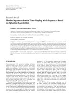
Figure 2: A three-stage model of CSF, based on implicit masking.
to a limited extent. The interac tion between the target and
the DC components should disappear when the spatial fre-
quency of the stimulus is high enough. In this case, there is

no effect of implicit masking. Therefore, the drop of con-
trast sensitivity because of implicit masking is restricted to
low spatial frequencies.
Second, this assumption offers an explanation of the ef-
fect of luminance on the contrast sensitivity at low spatial
frequencies; as mean luminance decreases, the component at
zero frequency decreases too. When this happens, other fac-
tors such as noise can dominate, and thus the relative atten-
uation at low f requencies decreases.
Third, this assumption also offers an explanation of the
dependence of the attenuation on temporal frequency [22].
The DC component of a grating is at zero temporal frequency
and zero spatial frequency in a 2D spatiotemporal frequency
domain, so the effects of implicit masking apply only to very
low temporal and spatial frequencies. Test gratings that are
modulated at high temporal frequencies would b e exempted
from the effect of implicit masking, no matter what the spa-
tial frequency of the grating is.
Finally, the effect of field size on contrast sensitiv ity can
be explained by the breadth of implicit masking. The extent
of implicit masking is determined by the spread of the DC
energy in the frequency domain. The larger the viewing field,
the less the spread [26]. This explains why the peak sensitiv-
ity shifts to lower spatial frequency as field size increases, ow-
ing to the decreasing breadth of implicit masking. The exact
amount of spread depends also on retinal inhomogeneities
[26].
Based on the concept of implicit masking, Yang et al. [24]
developed a quantitative model of the CSF. As schematized
in Figure 2, the form of visual processing is partitioned

into three functional stages. The first stage represents a
low-pass filter and it includes the effects of ocular optics,
photoreceptors, and neural summation. The second stage
represents a spread of grating energy to nearby frequencies.
This stage represents frequency spreading caused by in-
homogeneities in the stimulus, such as truncation of the
field, and spatial inhomogeneities in the visual system, such
as variation in the density of ganglion cells. The third
stage, a nonlinear thresholding operation, is characterized
by a nonlinear relationship between the required threshold
amplitude and the background amplitude values. When the
energy of the background field spreads to frequencies close
to 0 cpd, the v irtual masking amplitude at low frequencies
increases and so does the threshold amplitude [24]. In this
model, implicit masking is responsible for the CSF shape at
low spatial frequencies, and the low-pass filter determines
the sensitivity roll-off at high spatial frequencies. In a ddition
to the CSF shape, Figure 1 shows that the overall contrast
threshold reduces as the mean luminance level increases. It
was found that the inclusion of a photon-like shot noise, as
indicated in Figure 2, provided a satisfactory account of the
overall threshold changes [24]. The absolute shot noise in-
creases, but the noise contrast reduces with mean luminance
following a square-root law [27, 28].
In a further research, Yang and Stevenson [29]noticed
that the interocular luminance masking affects low, but not
high spatial frequencies, which suggests that the change of
visual sensitivity at high spatial frequencies is determined by
retinal processes, such as light adaptation, but not the lumi-
nance dependent noise.

So far the model is in an analytical form, taking pa-
rameter values, such as the frequency, the contrast, and
the luminance of the stimulus as model inputs. It can-
not, however, take stimulus profiles or images as the in-
puts. Later in this paper I will show how to extend such a
model to perform visual image processing with incorporat-
ing implicit masking and compressive nonlinear processes.
Nonlinearity and divisive normalization
Nonlinear processes in vision have often been explained by
a nonlinear transducer function [30, 31]. According to such
a theory, threshold is inversely proportional to the derivative
of the transducer function at any given pedestal amplitude
[2, 32, 33]. Heeger [34, 35] suggested that the nonlinear-
ity of the cells in striate cortex and related psychophysi-
cal data may be due to a normalization process. Foley [2]
suggested that such normalization requires inhibitory inputs
to the transducer function. However, specifying excitatory
and inhibitory interactions among different stimulus com-
ponents can be complicated in general cases. To deal with this
difficulty, I use locally pooled signals in either the space do-
main or the spatial frequency domain to replace the signal in
the denominator of the Naka-Rushton equation. Therefore,
such modified compressive nonlinearity can display some
features of divisive nor m alization.
2. IMAGE PROCESSING-BASED FRAMEWORK
The proposed model framework is based on the ideas of
implicit masking, modified compressive nonlinear process,
4 EURASIP Journal on Advances in Signal Processing
Visual
pattern

Low-pass
filter
Compressive
nonlinearity
Frequency
representation
Compressive
nonlinearity
Detection
Percept
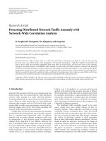
Figure 3: The schematized framework of visual image processing
for pattern detection and brightness perception. The output of the
last nonlinearity shows cortical information representation.
and other well-known properties of the visual system that
have been used in many models. The model components are
schematized in Figure 3, and are elaborated in the following
subsections.
Low-pass filtering
When the light modulating information of an image enters
into human eyes, it passes through the optical lens of the e ye
and is captured by photoreceptors in the retina. One func-
tion of photoreceptors is to sample the continuous spatial
variation of the image discretely. The cone signals are further
processed through horizontal cells, bipolar cells, amacrine
cells, and ganglion cells with some resampling. From an im-
age processing point of view, the effects of optical lens, sam-
pling, and resampling in the retinal mosaic are low-pass fil-
tering.
We estimate the front-end filter from psychophysical ex-
periments. It has been shown that the visual behavior at high

spatial frequencies follows an exponential curve [36]. Yang et
al. [24] extrapolated this relationship to low spatial frequen-
cies to describe the whole f ront-end filter with an exponential
function of spatial frequency:
LPF( f )
= Exp(−αf), (1)
where α is a parameter specifying the rate of attenuation for
a specific v iewing condition. Yang and Stevenson [37]mod-
ified the formula to account for the variation in α with the
mean luminance of the image:
α
= α
0
+
δ

L
0
,(2)
where α
0
and δ are two parameters and L
0
is the mean lumi-
nance of the image.
Retinal compressive nonlinearity
In the retina, there are several major layers of cells, starting
from photoreceptors including rods and three types of cones
to horizontal cells, bipolar cells, amacrine cells, and finally
to ganglion cells where the information is transmitted out

of the retina via optic nerve fibers to the central brain [38].
Retinal processes include a light adaptation, where the retina
becomes less sensitive if continuously exposed to bright light.
The adaptation effects are spatially localized [39, 40].
In the current model, the adaptation pools are assumed
to be constrained by ganglion cells with an aperture window:
W
g
(x, y) =
1
2πr
2
g
Exp

−
x
2
+ y
2
2r
2
g

,(3)
where r
g
is the standard deviation of the aperture. The adap-
tation signal at the level of ganglion cells I
g

is the convolution
of the low-passed input image I
c
with the window function
W
g
. In this algorithm, the window profile is approximated
as spatially invariant by considering only foveal vision. The
retinal signal I
R
is the output of a compressive nonlinearity.
The form of this nonlinear function is assumed here to be
the Naka-Rushton equation, which has been widely used in
models of retinal light adaptation [41, 42]. One major differ-
ence here is that the adaptation signal I
g
in the denominator
is a pooled signal, which is similar to a divisive normalization
process:
I
R
=
w
0

1+I
n
0

I

n
c
I
n
g
+

I
0
w
0

n
,(4)
where n and I
0
are parameters that represent the exponent
and the semisaturation constant of the Naka-Rushton equa-
tion, respectively, and w
0
is a reference luminance value. I n
conditions where I
c
and I
g
are all equal to w
0
, the retinal
output signal is the same as the input signal strength.
Cortical compressive nonlinearity

Simple cells and complex cells in the visual striate cortex
usually respond to stimuli of limited ranges in spatial fre-
quency and orientation [43, 44]. To capture this frequency
and orientation-specific nonlinearity, one can transform the
image I
R
from a spatial domain to a frequency domain rep-
resentation via a Fourier transform to T(f
x
, f
y
), which is then
divided by n
x
and n
y
to normalize the amplitude in the fre-
quency domain. Here f
x
and f
y
are the spatial frequencies in
x and y directions, respectively, and n
x
by n
y
is the number
of image pixels.
These cells also exhibit nonlinear properties; their fir-
ing rate does not increase until the stimulation strength

is above a threshold level and the firing rate saturates
when the stimulation strength is very strong [44]. In the
Jian Yang 5
model calculation, the signal in the frequency domain passes
through the same type of nonlinear compressive transform as
it did in the retinal processing. Following the concept of fre-
quency spread in implicit masking (see Figure 2), one major
step here is to compute the frequency spreading that affects
the masking signal in the denominator of the nonlinear for-
mula. In this model, the signal strength in the masking pool,
T
m
(f
x
, f
y
), is the convolution of the absolute signal amplitude
|T(f
x
, f
y
)| and an exponential window function:
W
c

f
x
, f
y


=
Exp

−
( f
2
x
+ f
2
y
)
0.5
σ

,(5)
where σ correlates with the extent of the frequency spreading
and the bandwidth of frequency channels. As the bandwidth
of frequency channels increases with the spatial frequency
[1], one should expect that the σ value increases with spa-
tial frequency. To simplify the computation, however, this
value is approximated as a fixed value in the current algo-
rithm. Applying the same form of compressive nonlinearity
as in the retina, the cortical signal in the frequency domain is
expressed as
T
c
= sign(T)
w
0


1+T
v
0

|T|
v
T
v
m
+

T
0
w
0

v
,(6)
where v and T
0
are parameters that represent the exponent
and the semisaturation constant of the Naka-Rushton equa-
tion for the cortical nonlinear compression, respectively. The
term T
m
in the denominator includes the energy spread of
the DC component (i.e., at 0 cpd) of the spatial pattern.
This component is processed in the same way as other fre-
quency maskers, if there are any, under (6). Thus, the concept
of implicit masking is naturally implemented in the image

processing framework. In summary, the major process in the
cortex is modeled by a compressive nonlinearity applying to
the spatial frequency and orientation components. The corti-
cal image representation in the frequency domain is given by
the function T
c
. This function will be used to calculate visual
responses for pattern detection and for estimating perceived
brightness, as described in the following sections.
3. MODEL FITS TO PATTERN DETECTION DATA
As mentioned earlier, this paper focuses on the nonlinear
parts of the visual process. In order to investigate whether
the model estimates pattern visibility reasonably, a detec-
tion stage was added in the model to fit existing experimen-
tal data. A simple Minkowski summation was used to esti-
mate the signal strength at a decision stage, although some
other approaches, such as linear summation within spatial
frequency channels [45], or signal detection theory [46, 47],
may ultimately turn out superior.
The following examples show model fits to two sets of ex-
perimental data on pattern detection performance. One set
data contains the contrast thresholds reported by Van Nes
and Bouman [16] for detecting gratings at various mean lu-
minance levels. The other set is from the Modelfest study
with the contrast thresholds of 43 patterns at a mean lumi-
nance level of about 30 cd/m
2
[45, 48].
Pattern detection stage
Based on the block diagram (Figure 3),avisualpattern

passes through a low-pass filter, a retinal compressive
nonlinearity, a frequency domain representation, and a cor-
tical compressive nonlinear ity to produce the cortical signal
as described by T
c
(see (6)). In real experiments, observers
look for the target signal against a background field. To sim-
ulate this task in the computation, one can calculate the cor-
tical visual response, T
c t
, in the spatial frequency domain in
respect to the visual pattern, and, T
c r
, to the reference back-
ground field. The signal strength in the detection stage is as-
sumed to be equal to the Minkowski summation of the dif-
ferences between T
c t
and T
c r
at every frequency component:
R
=

Δ f
x
Δ f
y
Σ


(T
c t
− T
c r

β

1/β
,(7)
where Δf
x
and Δf
y
are the frequency intervals along x
and y directions, respectively, and β is the exponent of
the Minkowski summation over different frequency compo-
nents. The response strength R is assumed to be a constant
value R
t
at a given threshold criterion.
Fits to Van Nes and Bouman data
The Van Nes and Bouman [16] paper reported the contrast
thresholds for detecting gratings with spatial frequencies in
the range of 0.5 to 48 cpd, covering 7 mean illuminance lev-
els in the range of 0.0009 to 900 trolands. The threshold val-
ues were measured using a method of limits, adjusting the
contrast value to make the test grating just visible or just dis-
appear to the observers. The major challenge for the compu-
tational model is to duplicate the thresholds, which change
with luminance and spatial frequency as shown in Figure 1.

There are total of 102 data points corresponding to gratings
of different spatial frequency and luminance combinations.
For each grating, the response strength R is determined
by (7). The model estimated contrast threshold is the one
that leads R to be equal to a constant R
t
value. Model pa-
rameters were optimized to minimize the root mean squared
(RMS) error between the model estimates and the experi-
mental data, both on a logarithmic scale:
E
=

Σ

log

C
i

− log

CE
i

2
n

1/2
. (8)

Here C
i
is the model estimated contrast threshold, CE
i
is the
contrast threshold reported by Van Nes and Bouman for the
ith stimulus, and n is 102 which is the number of data points
in the summation.
In model equations (1)to(7), there are 11 system pa-
rameters α
0
, δ, r
g
, w
0
, n, I
0
, v, T
0
, σ, β,andR
t
.Eachof
the parameters is a positive real number; and some of them
6 EURASIP Journal on Advances in Signal Processing
convey specific physical meaning about the visual system.
These parameter values can be estimated by optimizing the
fits between model predictions and experimental data. The
quality of the fits was not sensitive to some parameter values
when other parameters were optimized accordingly. These
parameters, δ, r

g
, w
0
,andβ,werethussetto0.10 deg td
1/2
,
0.9 min of arc, 100 cd/m
2
,and2.2, respectively, based on rea-
sonable pilot data fits. The other 7 parameters were opti-
mized to minimize the residual error as determined by (8).
The contrast thresholds of the fits are plotted in smooth
curves in Figure 1, where the RMS error being 0.10 log unit.
Although there is no bandpass filter built in the model,
the model output exhibits a bandpass behavior at high lu-
minance levels. This result demonstrates the role of implicit
masking. Furthermore, the model output c aptures the trend
of the threshold variation with spatial frequency and lumi-
nance nicely.
Fits to the Modelfest data
The above example shows that the model is adequate to cap-
ture visual performance on detecting the particular patterns,
that is, sinusoidal gratings. Now we examine how well this
model deals with a variety of patterns. Modelfest was a col-
laboration between many laboratories to measure contrast
thresholds of a broad range of patterns, including Gabor
functions of varying aspect ratio, Bessel and Gaussian func-
tions, lines, edges, checkerboard, natural scene, and random
noise, in order to provide a database for testing human vi-
sion models [45, 48]. There were 43 different monochro-

matic spatial patterns in the Modelfest test set. The field
size was 2.13
◦
× 2.13
◦
and mean background luminance was
about 30 cd/m
2
. The contrast thresholds were determined us-
ing two-alternative-forced-choice (2AFC) with 84% correct
responses.
The aim of developing a general purpose vision model
will be one step closer if the model can produce contrast
thresholds that are closely matched to the experimentally ob-
tained results for all the stimuli, without varying the above
determined model parameter values. To check this possibil-
ity, the luminance profile of each of the 43 visual stimuli
was input to the model algorithm to calculate their contrast
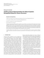
thresholds, which are shown in the dotted lines in Figure 4.
As a comparison, the circles show the mean experimental
data over 16 observers. Clearly, the model underestimates the
contrast thresholds in most of the cases. The model de via-
tion in terms of RMS error is 0.22 log unit. Taking into ac-
count the fact that the model parameters were obtained from
aquitedifferent experimental data set, the performance of
the model is encouraging.
Two areas were identified that could contribute to the
model deviations. One is on the low-pass filter. The Van Nes
and Bouman study used Maxwellian view with optical ap-
paratus, while the Modelfest study used direct view of video

displays. Thus it is reasonable to have a greater α
0
value in the
Modelfest study than that in the Van Nes and Bouman study.
The second area is the decision-making stage, as there were
differences in the threshold measurements. This may require
10
0
10
1
10
2
10
3
Contrast threshold
01020304050
Stimulus number
Figure 4: Contrast thresholds of 43 Modelfest stimuli. The data
points (circles) represent m ean experimental results over 16 ob-
servers; the dotted lines represent model predications with an RMS
error of 0.22 log unit; and the solid lines represent optimal model
fits with an RMS error of 0.11 log unit.
using different β and R
t
values in the current model. Con-
sequently, the solid lines in Figure 4 show the model fits to
the experimental data after optimizing the three par ameters
while the other 8 parameters were kept the same as in the pre-
vious case. The resulting RMS error is 0.11 log unit. The pa-
rameter value changed from 0.11 to 0.14 degree for α

0
,from
2.2to1.7forβ,andfrom0.36 to 0.53 for R
t
.
The RMS error is l arger than those reported by Watson
and Ahumada [45], however the current model has the ad-
vantage in dealing with diverse data sets. As discussed earlier,
this model can describe the luminance dependent CSFs. It
can a lso explain brightness perception as shown in the next
section.
From Figure 4, one can see that the major contribution
to the RMS error comes from stimuli #35 (a noise pattern)
and #43 (a natural scene), where the model estimates are
much lower than the experimental data as marked by the line
segments (see Figure 4). For the noise pattern, its spectra in
the spatial frequency domain have random phases. Including
a linear summation within narrow frequency channels can
cancel some of the energies due to the phase differences, thus
increasing the threshold estimate and potentially improving
the fit. For the natural scene, energy cancellation can happen
within linear channels too, due to the phase variations within
the summation windows.
4. SIMULATING BRIGHTNESS PERCEPTION
The current model algorithm is designed to deliver visual
information representation T
c
at a cortical level (see (6)).
This information can be used to estimate pattern visibility
as shown in the previous section. It is reasonable to believe

that the cortical information presentation can b e used to
Jian Yang 7
S
1
S
2
(a)
150
100
50
0
Amplitude (cd/m
2
)
012 345
X (deg)
S
1
S
2
(b)
Figure 5: Panel (a) is a demonstrative pattern to show the effect of simultaneous contrast, where stripe S
1
looks brighter than S
2
while they
have the same luminance, and panel (b) shows the luminance profile of the visual pattern (dotted lines) and the model simulation results of
the brightness before (dim lines) and after (thick lines) a fill-in process.
produce visual perception too when additional processes are
included. In this section, I will show that the obtained cor-

tical representation , after adding a fill-in process, can also
be used to estimate the brightness perception of three well-
know examples: simultaneous contrast, assimilation, and
crispening .
Local simultaneous contrast
It is well known that the brightness of a visual target de-
pends not only on the luminance of the target, but also on
the local contrast of its edges in reference to the luminance
of adjacent areas. Simultaneous contrast is often demon-
strated by the brightness of a gray spot at different sur-
rounding luminance levels (e.g., [49]). Although the lumi-
nance level of the gray spot is fixed, the perceived brightness
of the spot increases while the surrounding luminance de-
creases.
For simplicity, the examples shown here are for one-
dimensional patterns.
1
In the first example, the visual pattern
with simultaneous contrast is demonstrated in Figure 3.Even
though both of the stripes S
1
and S
2
have the same luminance
level of about 50 cd/m
2
(see the dotted lines in panel (b) of
Figure 5 for the corresponding luminance profile), stripe S
1
that is flanked by a lower luminance level of about 25 cd/m

2
looks brighter than stripe S
2
that is flanked by a higher lumi-
nance level of about 100 cd/m
2
. This has been attributed to
the effect of local contrast.
In the model simulation of the perceived brightness, the
luminance profile of the visual pattern is fed into the model
1
Note: the visual patterns in Figures 5–7 are for the demonstrative purpose.
The pattern luminance will not match the specified luminance profiles
due to media limitation and the lack of standards to calibrate the printed
or displayed images. Therefore, the perceived brightness by readers here
may not reflect what it should be as in well-controlled experiments.
algorithm as an input. Based on (1)to(6), one can ob-
tain the frequency domain representation, that is, T
c
, of the
visual pattern. By performing an inverse FFT, one obtains
the spatial representation of the pattern as shown by the
dim lines in Figure 5(b). This spatial response contains over-
shoots near the edges. For estimating the brightness of each
stripe, some investigators have suggested a fill-in process
[50, 51] or an averaging process [4]. The thick lines in
Figure 5(b) are the average values of the dotted lines within
each stripe after considering such a simple fill-in process. As
the final simulation results (thick lines) show, the visual re-
sponse to the left-side stripe is 105 that is larger than the re-

sponse of 66 to the right-side stripe, in agreement with our
perceptintermsthatS
1
is perceived brighter than S
2
.Asa
clarification, this paper provides only qualitative compari-
son of the model prediction to actual visual percept; no ef-
forts have been taken to attain an adequate match in num-
bers. The unit of brightness perception from the model has
not provided a clear meaning yet, and the scale relies on the
model parameter w
0
, which was set to 100 cd/m
2
in the cur-
rent model algorithm as mentioned earlier.
Long range assimilation
The simultaneous contrast in the above example demon-
strates the effect of local contrast on brightness percep-
tion. It has been shown in the literature that l onger range
interactions, other than local contrast, can also influence
brightness perception as exampled by assimilation [52, 53].
Here, the perceived brightness is affected by the luminance
level of nonadjacent background areas. The visual patterns
on panels (a) and (c) of Figure 6 is a variant version of the
bipartite field in [52,Figure1].Inthispattern,bothstripes
S
1
and S

2
have a same luminance of 97 cd/m
2
, and their ad-
jacent flanking stripes have a same luminance of 48 cd/m
2
.
ThedottedlinesofFigures6(c) and 6(d) show their lumi-
nance profiles. The percept of stripe S
1
being brighter than
8 EURASIP Journal on Advances in Signal Processing
S
1
(a)
S
2
(b)
150
100
50
0
Amplitude (cd/m
2
)
012345
X (deg)
S
1
(c)

150
100
50
0
Amplitude (cd/m
2
)
012345
X (deg)
S
2
(d)
Figure 6: Panels (a) and (c) show two patterns to demonstrate the effect of assimilation, where stripe S
1
looks brighter than S
2
while they
have the same luminance value, and panels (b) and (d) show the luminance profile of the middle part 5 degrees of the patterns (dotted lines),
and the corresponding model estimated brightness (thick lines) after a fill-in process.
stripe S
2
cannot be explained by local contrast as there is
no difference in local contrast. The only difference between
the two patterns is the luminance levels of the non-adjacent
background fields, which are 25 cd/m
2
in A and 86 cd/m
2
in B. Such longer range effect was attributed to assimilation
[52].

The model calculation follows the same way as described
in the preceding example. Each of the luminance profiles of
the patterns is fed into the model as an input to calculate its
cortical representation. The simulated brightness following
the fill-in process for pattern A is shown as the thick lines
in Figure 6(c) where stripe S
1
has a value of 141, and that
for pattern B is shown as the thick lines in Figure 6(d) where
stripe S
2
has a value of 124. Therefore, the model predicts
that stripe S
1
isperceivedbrighterthanstripeS
2
by 17 units,
which is consistent w ith our percepts in terms that stripe S
1
is likely perceived brighter than S
2
.
Crispening effect
Let us consider one more example here. It has been shown
that the perceived brightness of a spot changes more rapidly
with the luminance of the spot when its luminance is closer to
the surrounding luminance [54]. Such crispening can also be
demonstrated by seeing the effect of background luminance
on the brightness difference of two spots (e.g., see [55]). The
perceived difference is the largest when the background lumi-

nance value is somewhere between the luminance values of
the two spots. As illustrated in Figure 7, the brightness differ-
ence between stripes S
1
and T
1
is barely detectable, while the
difference between stripes S
2
and T
2
is easier to see, although
S
1
and S
2
have the same luminance of 57 cd/m
2
and T
1
and
T
2
have the same luminance of 48 cd/m
2
. The dotted lines
in Figure 7(c) represent the luminance profile of Figure 7(a)
and the dotted lines of Figure 7(d) represent the profile of
Figure 7(b).
In the same way as in previous two examples, the lu-

minance profile of each pattern is entered into the model
algorithm to calculate its cortical representation, and then
through a fill-in process. The thick lines of Figure 7(c)
represent the model predicted brightness for seeing pat-
tern A, and the thick lines of Figure 7(d) represent the
brightness for seeing pattern B. For a comparison, the
model estimated brightness difference between S
1
and T
1
,
which is 11 units, is less than the difference between S
2
and T
2
, which is 14 units. Thus, the model outputs are
qualitatively consistent with the perceived brightness differ-
ences.
Jian Yang 9
S
1
T
1
(a)
S
2
T
2
(b)
140

120
100
80
60
40
Amplitude (cd/m
2
)
012345
X (deg)
S
1
T
1
(c)
140
120
100
80
60
40
Amplitude (cd/m
2
)
012345
X (deg)
S
2
T
2

(d)
Figure 7: Stripes S
1
and S
2
have the same luminance of 57 cd/m2; stripes T
1
and T
2
have the same luminance of 48 cd/m2; and the
background luminance is 17 cd/m2 for pattern A and 54 cd/m2 for pattern B. Model predicted brightness for stripes S
1
and T
1
is 123 and
112 (thick lines of panel (c)), with a difference of 11 units, and the predicted brightness for stripes S
2
and T
2
is 96 and 82 (thick lines of panel
(d)), with a difference of 14 units.
The three examples show that the current model can
describe the effects of both local contrast and assimilation
under a common theoretical framework. As a same algo-
rithm and a same set of parameter values were used in each
case, it is an encouraging evidence of showing the generality
of the developed human vision model.
5. SUMMARY
Differing from most existing vision models, the current ap-
proach does not use CSF as the front-end filter in model-

ing visual image processing. Instead, the model simulates the
CSF behavior at varying mean luminance by implementing
implicit masking, using very basic components of visual im-
age processing. They include a front-end low-pass filter, a
nonlinear compressive process in the retina performed in the
spatial domain, and a nonlinear compressive process in the
cortex performed in the frequency domain.
After including Minkowski summation in the deci-
sion stage, this model can describe the contrast thresh-
olds obtained in two prominent and very different studies,
namely the luminance dependent CSFs [16] and the Mod-
elfest data [45, 48]. The residual RMS errors between the
model and experimental data were about 0.1 log unit. It also
suggests that further model improvement could be reached
by applying more appropriate decision-making roles such as
adding linear frequency channels.
The same model can be used to identify the direction of
visual illusion with respect to the change of perceived bright-
ness in simultaneous contrast, assimilation, and crispen-
ing effect. While reports in the literature have shown that
brightness perception can be simulated using the local en-
ergy model of feature detection [56, 57], frequency chan-
nels [5, 58, 59], or natural scene statistics [60], the current
approach relies on compressive nonlinear processes at both
retina and visual cortex. Both Blakeslee et al. [59] and Dakin
and Bex [60] use a frequency weight that increases with spa-
tial frequency, in a way attenuating low frequency compo-
nents. Similarly, the current model applies a concept of im-
plicit masking to attenuate low frequency. The major differ-
ences here are that the amount of attenuation depends on the

mean luminance level, and that frequency masking and spa-
tially localized adaptation are included. It remains to see how
important it is to apply these treatments in future studies. It
is, nevertheless, encouraging to see the generality of the de-
veloped model, which integrates the three diverse perceptual
phenomena under a common theoretical framework, in ad-
dition to its capability of estimating pattern visibility in a
10 EURASIP Journal on Advances in Signal Processing
variety of conditions. In further studies, we need to concen-
trate on quantitative matches between the model predictions
and experimental data on brightness perception.
ACKNOWLEDGMENTS
The author thanks Professor Walter Makous of the Univer-
sity of Rochester and Professor Scott Stevenson of the Uni-
versity of Houston for their helpful discussion regarding
implicit masking in early years. The author thanks Profes-
sor Adam Reeves of Northeastern University and two anony-
mous reviewers for their helpful comments and suggestions.
REFERENCES
[1] H. R. Wilson, D. K. McFarlane, and G. C. Phillips, “Spatial
frequency tuning of orientation selective units estimated by
oblique masking,” Vision Research, vol. 23, no. 9, pp. 873–882,
1983.
[2] J. M. Foley, “Human luminance pattern-vision mechanisms:
masking experiments required a new model,” Journal of the
Optical Society of America A, vol. 11, no. 6, pp. 1710–1719,
1994.
[3] A. B. Watson and J. A. Solomon, “A model of visual contrast
gain control and pattern masking ,” Journal of the Optical Soci-
ety of America A, vol. 14, no. 9, pp. 2379–2391, 1997.

[4] E. G. Heinemann and S. Chase, “A quantitative model for
simultaneous brightness induction,” Vision Research, vol. 35,
no. 14, pp. 2007–2020, 1995.
[5] J. McCann, “Gestalt vision experiments from an image pro-
cessing perspective,” in Proceedings of the Image Processing, Im-
age Quality, Image Capture Systems Conference (PICS ’01),pp.
9–14, Montreal, Quebec, Canada, April 2001.
[6] J. Yang, “Approaching a unified model of pattern detection and
brightness perception,” in Human Vision and Electronic Imag-
ing VII, vol. 4662 of Proceedings of SPIE, pp. 84–95, San Jose,
Calif, USA, January 2002.
[7] G. L. Fain and M. C. Cornwall, “Light and dark adaptation
in vertebrate photoreceptors,” in Contrast Sensitivity,R.Shap-
ley and D. M K. Lam, Eds., pp. 3–32, MIT Press, Cambridge,
Mass, USA, 1993.
[8] R. Shapley, E. Kaplan, and K. Purpura, “Contrast sensitivity
and light adaptation in photoreceptors in the retinal network,”
in Contrast Sensitivity, R. Shapley and D. M K. Lam, Eds., pp.
103–116, MIT Press, Cambridge, Mass, USA, 1993.
[9] N.V.S.Graham,Visual Pattern Analyzers, Oxford University
Press, New York, NY, USA, 1989.
[10] A. B. Watson, “Efficiency of a model human image code,” Jour-
nal of the Optical Societ y of America A, vol. 4, no. 12, pp. 2401–
2417, 1987.
[11] E. Peli, “Contrast in complex images,” Journal of the Optical
Society of America A, vol. 7, no. 10, pp. 2032–2040, 1990.
[12] E. Peli, “Limitations of image enhancement for the visually
impaired,” Optometry and Vision Science, vol. 69, no. 1, pp.
15–24, 1992.
[13] S. Daly, “The visible difference predictor: an algorithm for the

assessment of image fidelity,” in Human Vision, Visual Process-
ing, and Digital Display III, vol. 1666 of Proceedings of SPIE,
pp. 2–15, San Jose, Calif, USA, February 1992.
[14] J. Lubin, “A visual discrimination model for imaging system
design and evaluation,” in Vision Models for Target Detection
and Recognition, E. Peli, Ed., pp. 245–283, World Scientific,
River Edge, NJ, USA, 1995.
[15] O. H. Schade, “Optical and photoelectric analog of the eye,”
Journal of the Optical Society of America, vol. 46, no. 9, pp. 721–
739, 1956.
[16] F. L. Van Nes and M . A. Bouman, “Spatial modulation transfer
in the human eye,” Journal of the Optical Society of America,
vol. 57, no. 3, pp. 401–406, 1967.
[17] F. W. Campbell and J. G. Robson, “Application of Fourier anal-
ysis to the visibility of gratings,” Journal of Physiology, vol. 197,
no. 3, pp. 551–566, 1968.
[18] B. A. Wandell, Foundations of Vision, Sinauer Associates, Sun-
derland, UK, 1995.
[19] P. G. J. Barten, “Physical model for the contrast sensitivity of
the human eye,” in Human Vision, Visual Processing, and Digi-
tal Display III, vol. 1666 of Proceedings of SPIE, pp. 57–72, San
Jose, Calif, USA, February 1992.
[20] P. G. J. Barten, Contrast Sensitivity of the Human Eye and
Its Effects on Image Quality, SPIE Optical Engineering Press,
Bellingham, Wash, USA, 1999.
[21] J. Rovamo, J. Mustonen, and R. N
¨
as
¨
anen, “Modelling con-

trast sensitivity as a function of retinal illuminance and grating
area,” Vision Research, vol. 34, no. 10, pp. 1301–1314, 1994.
[22] J. Yang and W. Makous, “Spatiotemporal separ ability in con-
trast sensitivity,” Vision Research, vol. 34, no. 19, pp. 2569–
2576, 1994.
[23] J. Yang and W. Makous, “Modeling pedestal experiments with
amplitude instead of contrast,” Vision Research, vol. 35, no. 14,
pp. 1979–1989, 1995.
[24] J. Yang, X. Qi, and W. Makous, “Zero frequency masking and a
modelofcontrastsensitivity,”Vision Research, vol. 35, no. 14,
pp. 1965–1978, 1995.
[25] W. L. Makous, “Fourier models and the loci of adaptation,”
Journal of the Optical Society of America A,vol.14,no.9,pp.
2323–2345, 1997.
[26] J. Yang and W. Makous, “Implicit masking constrained by
spatial inhomogeneities,” Vision R esearch, vol. 37, no. 14, pp.
1917–1927, 1997.
[27] J. Krauskopf and A. Reeves, “Measurement of the effect of pho-
ton noise on detection,” Vision Research,vol.20,no.3,pp.
193–196, 1980.
[28] A.Reeves,S.Wu,andJ.Schirillo,“Theeffect of photon noise
on the detection of white flashes,” Vision Research, vol. 38,
no. 5, pp. 691–703, 1998.
[29] J. Yang and S. B. Stevenson, “Post-retinal processing of back-
ground luminance,” Vision Research, vol. 39, no. 24, pp. 4045–
4051, 1999.
[30] J. Nachmias and R. V. Sansbur y, “Grating contrast: discrimi-
nation may be better than detection,” Vision Research, vol. 14,
no. 10, pp. 1039–1042, 1974.
[31] J. M. Foley and G. E. Legge, “Contrast detection and near-

threshold discrimination in human vision,” Vision Research,
vol. 21, no. 7, pp. 1041–1053, 1981.
[32] G. E. Legge and J. M. Foley, “Contrast masking in human vi-
sion,” Journal of the Optical Society of America, vol. 70, no. 12,
pp. 1458–1471, 1980.
[33] J. Ross and H. D. Speed, “Contrast adaptation and contrast
masking in human vision,” Proceedings of the Royal Society of
London B: Biological Sciences, vol. 246, no. 1315, pp. 61–70,
1991.
[34] D. J. Heeger, “Normalization of cell responses in cat striate cor-
tex,” Visual Neuroscience, vol. 9, no. 2, pp. 181–197, 1992.
Jian Yang 11
[35] D. J. Heeger, “The representation of visual stimuli in pri-
mar y visual cortex,” Current Directions in Psychological Science,
vol. 3, no. 5, pp. 159–163, 1994.
[36] F. W. Campbell, J. J. Kulikowski, and J. Levinson, “The effect
of orientation on the visual resolution of gratings,” Journal of
Physiology, vol. 187, no. 2, pp. 427–436, 1966.
[37] J. Yang and S. B. Stevenson, “Effect of background components
on spatial-frequency masking,” Journal of the Optical Society of
America A, vol. 15, no. 5, pp. 1027–1035, 1998.
[38] R. W. Rodieck, The Vertebrate Retina,W.H.Freeman,San
Francisco, Calif, USA, 1973.
[39] D. I. A. MacLeod, D. R. Williams, and W. Makous, “A vi-
sual nonlinearity fed by single cones,” Vision Research, vol. 32,
no. 2, pp. 347–363, 1992.
[40] S. He and D. I. A. Macleod, “Contrast-modulation flicker: dy-
namics and spatial resolution of the light adaptation process,”
Vision Research, vol. 38, no. 7, pp. 985–1000, 1998.
[41] R. M. Boynton and D. N. Whitten, “Visual adaptation in

monkey cones: recordings of late receptor potentials,” Scie nce,
vol. 170, no. 965, pp. 1423–1426, 1970.
[42] J. E. Dowling, The Retina: An Approachable Part of the Brain,
The Belknap Press of Harvard Universiyt Press, Cambridge,
Mass, USA, 1987.
[43] R. Shapley and P. Lennie, “Spatial frequency analysis in the
visual system,” Annual Review of Neuroscience, vol. 8, pp. 547–
583, 1985.
[44]R.L.DeValoisandK.K.DeValois,Spatial Vision,Oxford
University Press, New York, NY, USA, 1988.
[45]A.B.WatsonandA.J.AhumadaJr.,“Astandardmodelfor
foveal detection of spatial contrast,” Journal of Vision, vol. 5,
no. 9, pp. 717–740, 2005.
[46] W. S. Geisler, “Sequential ideal-observer analysis of visual dis-
criminations,” Psychological Review, vol. 96, no. 2, pp. 267–
314, 1989.
[47] M. P. Eckstein, C. K. Abbey, and F. O. Bochud, “A practical
guide to model observers for visual detection in synthetic and
natural noise images,” in The Handbook of Medical Imaging,
Vol. 1, J. Beutel, H. L. Kundel, and R. L. Van Metter, Eds.,
Progress in Medical Physics and Psychophysics, pp. 593–628,
SPIE Press, Bellingham, Wash, USA, 2000.
[48] T. Carney, S. A. Klein, C. W. Tyler, et al., “The development of
an image/threshold database for designing and testing human
vision models,” in Human Vision and Electronic Imaging IV,
vol. 3644 of Proceedings of SPIE, pp. 542–551, San Jose, Calif,
USA, January 1999.
[49] E. Hering, Outlines of a Theory of the Light Sense, Harvard Uni-
versity Press, Cambridge, Mass, USA, 1964.
[50] L. E. Arend and R. Goldstein, “Lightness models, gr adient il-

lusions, and curl,” Perception and Psychophysics,vol.42,no.1,
pp. 65–80, 1987.
[51] S. Grossberg and D. Todorovi
´
c, “Neural dynamics of 1-D and
2-D brightness perception: a unified model of classical and re-
cent phenomena,” Perception and Psychophysics, vol. 43, no. 3,
pp. 241–277, 1988.
[52] R. Shapley and R. C. Reid, “Contrast and assimilation in the
perception of brightness,” Proceedings of the National Academy
of Sciences of the United States of America, vol. 82, no. 17, pp.
5983–5986, 1985.
[53] S. S. Shimozaki, M. P. Eckstein, and C. K. Abbey, “Spa-
tial profiles of local and nonlocal effects upon contrast
detection/discrimination from classification images,” Journal
of Vision, vol. 5, no. 1, pp. 45–57, 2005.
[54] H. Takasaki, “Lightness change of grays induced by change in
reflectance of gray background,” Journal of the Optical Society
of America, vol. 56, no. 4, pp. 504–509, 1966.
[55] M. D. Fairchild, Color Appearance Models, Addison-Wesley,
Reading, Mass, USA, 1998.
[56] M. C. Morrone and D. C. Burr, “Feature detection in hu-
man vision: a phase-dependent energy model,” Proceedings
of the Royal Society of London B: Biological Sciences, vol. 235,
no. 1280, pp. 221–245, 1988.
[57] M. C. Morrone, D. C. Burr, and J. Ross, “Illusory brightness
step in the Chevreul illusion,” Vision Research, vol. 34, no. 12,
pp. 1567–1574, 1994.
[58] J. A. McArthur and B. Moulden, “A two-dimensional model of
brightness perception based on spatial filtering consistent with

retinal processing,” Vision Research, vol. 39, no. 6, pp. 1199–
1219, 1999.
[59] B. Blakeslee, W. Pasieka, and M. E. McCourt, “Oriented mul-
tiscale spatial filtering and contrast normalization: a parsimo-
nious model of brightness induction in a continuum of stim-
uli including White, Howe and simultaneous brightness con-
trast,” Vision Research, vol. 45, no. 5, pp. 607–615, 2005.
[60] S. C. Dakin and P. J. Bex, “Natural image statistics mediate
brightness ‘filling in’,” Proceedings of the Royal Society of Lon-
donB:BiologicalSciences, vol. 270, no. 1531, pp. 2341–2348,
2003.
Jian Yang received a B.S. degree in ph ysics
from Fudan University in 1982, an M.S.
degree in optics from the Shanghai Insti-
tute of Optics and Fine Mechanics in 1984,
a Ph.D. degree in experimental psychology
from Northeastern University in 1991, and
postdoctoral training in visual science at the
University of Rochester. Then he worked as
a Research Associate at the University of
Houston pursuing human vision research,
and as a Principal Scientist at Eastman Kodak Company conduct-
ing applied research in image quality and image science. He is cur-
rently providing consulting services on human factors issues, hu-
man vision-based e valuation and optimization in imaging product
design, development of computational algorithms to estimate hu-
man visual per formance, development of automated tools to mon-
itor the image quality of imaging products, perceptual experimen-
tal designs, and quantitative analysis and mathematical modeling
of vision experimental data. He holds 3 US patents and has coau-

thored over 30 scientific papers.