Báo cáo hóa học: " Research Article Classification of Underlying Causes of Power Quality Disturbances: Deterministic versus Statistical Methods" doc

Hindawi Publishing Corporation
EURASIP Journal on Advances in Signal Processing
Volume 2007, Article ID 79747, 17 pages
doi:10.1155/2007/79747
Research Article
Classification of Underlying Causes of Power Quality
Disturbances: Deterministic versus Statistical Methods
Math H. J. Bollen,
1, 2
Irene Y. H. Gu,
3
PeterG.V.Axelberg,
3
and Emmanouil Styvaktakis
4
1
STRI AB, 771 80 Ludvika, Sweden
2
EMC-on-Site, Lule
˚
a University of Technology, 931 87 Skellefte
˚
a, Sweden
3
Department of Signals and Systems, Chalmers University of Te chnology, 412 96 Gothenburg, Sweden
4
The Hellenic Transmission System Operator, 17122 Athens, Greece
Received 30 April 2006; Revised 8 November 2006; Accepted 15 November 2006
Recommended by Mois
´
es Vidal Ribeiro

This paper presents the two main types of classification methods for power quality disturbances based on underlying causes:
deterministic classification, giving an expert system as an example, and statistical classification, with support vector machines (a
novel method) as an example. An expert system is suitable when one has limited amount of data and sufficient power system
expert knowledge; however, its application requires a set of threshold values. Statistical methods are suitable when large amount
of data is available for training. Two important issues to guarantee the effectiveness of a classifier, data segmentation, and feature
extraction are discussed. Segmentation of a sequence of data recording is preprocessing to partition the data into segments each
representing a duration containing either an event or a transition between two events. Extraction of features is applied to each
segment individually. Some useful features and their effectiveness are then discussed. Some experimental results are included for
demonstrating the effectiveness of both systems. Finally, conclusions are given together with the discussion of some future research
directions.
Copyright © 2007 Hindawi Publishing Corporation. All rights reserved.
1. INTRODUCTION
With the increasing amount of measurement data from
power quality monitors, it is desirable that analysis, charac-
terization, classification, and compression can be performed
automatically [1–3]. Further, it is desirable to find out the
cause of each disturbance, for example, whether a voltage
dip is caused by a fault or by some other system event such
as motor starting or transformer energizing. Designing a ro-
bust classification for such an application requires interdis-
ciplinary research, and requires efforts to bridge the gap be-
tween power engineering and signal processing. Motivated
by the above, this paper describes two different types of auto-
matic classification methods for power quality disturbances:
expert systems and support vector machines.
There already exists a significant amount of literature
on automatic classification of power quality disturbances,
among others [4–24]. Many techniques have further been de-
veloped for extracting features and characterization of power
quality disturbances. Feature extraction may apply directly

to the original measurements (e.g., RMS values), from some
transformed domain (e.g. , Fourier and wavelet transforms,
and subband filters) or from the parameters of signal models
(e.g., sinusoid models, damped sinusoid models, AR mod-
els). These features may be combined with neural networks,
fuzzy logic, and other pattern recognition methods to yield
classification results.
Among the proposed methods, only a few systems have
shown to be significant in terms of being highly relevant
and essential to the real world problems in power systems.
For classification and characterizing power quality measure-
ments, [6, 15, 16] proposed a classification using wavelet-
based ANN, HMM, and fuzzy systems; [19, 20] proposed an
event-based expert system by applying e vent/transient seg-
mentation and rule-based classification of features for differ-
ent events; and [13] proposed a fuzzy expert system. Each
of these methods is shown to be suitable for one or several
applications, and is promising in certain aspects in the appli-
cations.
1.1. Some general issues
Despite the variety of classification methods, two key issues
are associated with the success of any classification system.
2 EURASIP Journal on Advances in Signal Processing
v(t)
i(t)
Segmen-
tation
Event
segments
Transition

segments
Feature
extraction
Additional
processing
Features
Classifi-
cation
Class
Figure 1: The processes of classification of power quality distur-
bances.
(i) Properly handling the data recordings so that each in-
dividual event (the term “event segment” will be used
later) is associated with only one (class of) underlying
cause. The situation were one event (segment) is due
to a sequence of causes should be avoided.
(ii) Selecting suitable features that make the underlying
causes effectively distinguishable from each other. It is
counter-productive to use features that have the same
range of values for all classes.
Extracting “good” features is strongly dependent on the
available power system expertise, even for statistical classi-
fiers. There exists no general approach on how the features
should be chosen.
It is worth to notice a number of other issues that are
easily forgotten in the design of a classifier. The first is that
the goal of the classification system must be well formu-
lated: is it aimed at classifying the type of voltage distur-
bance, or the underly ing causes of the disturbances? It is a
common mistake to mix the types of voltage disturbance

(or phenomena) and their underlying causes. The former
can be observed directly from the measurements, for ex-
ample, interruption, dip, and standard classification meth-
ods often exist. Wh ile determining, the latter is a more dif-
ficult and challenging task (e.g., dip caused by fault, trans-
former energizing), and is more important for power sys-
tem diagnostics. Finding the underlying causes of distur-
bances not only requires signal analysis, but often also re-
quires the information of power network configuration or
settings. Further, many proposed classification methods are
verified by using simulations in a power-system model. It is
important to notice that these models should be meaningful,
consistent, and close to reality. Deviating from such a prac-
tice may make the work irrelevant to any practical applica-
tion.
It is important to emphasize the integration of essential
steps in each individual classification system as outlined in
the block diagram of Figure 1.
Before the actual classification can take place, appropriate
features have to be extrac ted as input to the classifier. Seg-
mentation of the voltage and/or current recordings should
take place first, after which features are mainly obtained from
the event segments, with additional information from the
processing of the transition segments.
1.2. Deterministic and statistical classifiers
This paper concentrates on describing the deterministic and
statistical classification methods for power system distur-
bances. Two automatic classification methods for power
quality disturbances are described: expert systems as a deter-
ministic classification example, and support vector machines

as a statistical classification example.
(i) Rule-based expert systems form a deterministic clas-
sification method. This method finds its application when
there is a limited amount of data available, however, there
exists good prior knowledge from human experts (e.g., from
previously accumulated experience in data analysis), from
which a set of rules can be created based on some previous
expertise to make a decision on the origins of disturbances.
The performance of the classification i s much dependent on
the expert rules and threshold settings. The system is simple
and easy to implement. The disadvantage is that one needs to
fine tune a set of threshold values. The method fur ther leads
to a binary decision. There is no probability on whether the
decision is right or wrong or on the confidence of the deci-
sion.
(ii) Support vector machine classifiers are based on the
statistical learning theory. The method is suitable for appli-
cations when there are large amounts of training data avail-
able. The advantages include, among others, that there are
no thresholds to be determined. Further, there is a guaran-
teed upper bound for the generalization performance (i.e.,
the performance for the test set). The decision is made based
on the learned statistics.
1.3. Structure of the paper
In Section 2, segmentation methods, including model resid-
ual and RMS sequence-based methods, are described.
Through examples, Section 3 serves as the “br idge” that
translates the physical problems and phenomena of power
quality disturbances using power system knowledge into sig-
nal processing “language” where feature-based data char-

acterization can then be used for distinguishing the un-
derlying causes of disturbances. Section 4 describes a rule-
based expert system for classification of voltage disturbances,
as an example of deterministic classification systems. Next,
Section 5 presents the statistical-based classification method
using support vector machines along with a novel proposed
method, which serves as an example of the statistical classifi-
cation systems. Some conclusions are then given in Section 6.
2. SEGMENTATION OF VOLTAGE WAVEFORMS
For analyzing power quality disturbance recordings, it is
essential to partition the data into segments. Segmentation,
which is widely used in speech signal processing [25], is
found to be very useful as a preprocessing step towards an-
alyzing power quality disturbance data. The purpose of the
segmentation is to divide a data sequence into stationary and
nonstationary parts, so that each segment only belongs to
one disturbance event (or one part of a disturbance event)
which is caused by a single underlying reason. Depending
Math H. J. Bol len et al. 3
on whether the data within a segment is stationarit y, dif-
ferent signal processing strategies can then be applied. In
[20], a ty pical recording of a fault-induced voltage dip is
split into three segments: before, dur ing, and after the fault.
The divisions between the segments correspond to fault ini-
tiation and fault clearing. For a dip due to motor starting,
the recording is split to only two segments: before and af-
ter the actual starting instant. The starting current (and thus
the voltage drop) decays gradually and smoothly towards the
new steady state.
Figure 2 shows several examples where the residuals of

Kalman filter have been used for the segmentation. The
segmentation procedure divides the voltage waveforms into
parts with well-defined characteristics.
2.1. Segmentation based on residuals from
the data model
One way to segment a given disturbance recording is to use
the model residuals, for example, the residuals from a si-
nusoid model, or an AR model. The basic idea behind this
method is that when a sudden disturbance appears, there will
be a mismatch in the model, which leads to a large model er-
ror (or residual). Consider the harm onic model to describe
the voltage waveform:
z(n)
=
N

k=1
A
i
cos

2πnf
k
+ φ
k

+ v(n), (1)
where f
k
= 2πkf

0
/f
s
is the kth harmonic frequency, f
0
is as-
sumed to be the power system fundamental frequency, and
f
s
the sample frequency. Here, the model order N should be
selected according to how many harmonics are required to
accommodate as being nonsignificant disturbances.
To detect the transition points, the following measure of
change is defined and used to extract the average Kalman fil-
ter residual e(n)
= z(n) − z(n) within a short window of size
w as follows:
d(n)
=

1
w
n+w/2

i=n−w/2

z(i) − z(i)


2

,(2)
where
z(n) is the estimate z(n) from the Kalman filter. If d(n)
is prominent, there is a mismatch between the signal and
the model and a transition point is assumed to have been
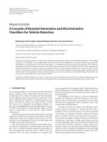
detected. Figure 3 shows an example where the transition
points were extracted by utilizing the residuals of a Kalman
filter of N
= 20. This is a recording of a multistage voltage
dip as measured in a medium voltage network.
The detection index d(n) is obtained by using the resid-
uals of three Kalman filters (one for each phase). Then the
three detection indices are combined into one by consider-
ing at each time instant the largest of the three indices. In
such a way, the recordings are split to event segments (where
the detection index is low) and transition segments (where the
detection index is high). The order of Kalman filters is se-
lected as being able to accommodate the harmonics that are
caused by events like transformer saturation or arcing, which
was suggested as N
= 20 in [20].
2.2. Segmentation based on time-dependent
RMS sequences
In case only RMS voltage versus time is available, segmen-
tation remains possible with these time-dependent RMS se-
quence as input. An RMS sequence is defined as
V
RMS

t

k

=





1
N
t
k

t=t
k−N+1
v
2
(t), t
k
= t
0
, t
1
, ,(3)
where v(t
k
) is the voltage/current sample, and N is the size
of the sliding window used for computing the RMS. Rms
sequence-based segmentation uses a similar strategy as the
method discussed above; however the measure of change is

computed from the derivatives of RMS values instead of from
model residuals. The segmentation can be described by the
following steps.
(1) Downsampling an RMS sequence
Since the time-resolution of an RMS sequence is low and the
difference between two consecutive RMS samples is relatively
small, the RMS sequence is first downsampled before com-
puting the der ivatives. This wil l reduce both the sensitivity of
the segmentation to the fluctuations in RMS derivatives and
the computational cost. In general, an RMS sequence with a
larger downsample rate will result in fewer false segments (or
split of segments) however with a lower time resolution of
segment boundaries. Conversely, for an RMS sequence with
a smaller downsample rate, the opposite holds. Practically
the downsample rate m is often chosen empirically, for ex-
ample, for the examples in this subsection, m
∈ [N/16, N]
is chosen (N is the number of RMS samples in one cycle).
In many cases only a limited number of RMS values per cy-
cle are stored (two according to the standard method in IEC
61000-4-30) so that further downsampling is not needed. For
notational convenience we denote the downsampled RMS se-
quence as
V
RMS


t
k


,

t
k
=
t
k
m
. (4)
(2) Computing the first-order derivatives
A straightforward way to detect the segmentation boundaries
is from the changes of RMS values, for example, using the
first-order derivative
M
j
RMS


t
k

=


V
j
RMS


t

k

− V
j
RMS


t
k−1



,(5)
where j
= a, b, c indicate the different phases. Consider ei-
ther a single-phase or a three-phase measurement, the mea-
sure of changes M
RMS
inRMSvaluesisdefinedby
M
RMS


t
k

=
⎧
⎨
⎩

M
a
RMS


t
k

for 1 phase,
max

M
a
RMS
, M
b
RMS
, M
c
RMS


t
k

for 3 phases.
(6)
4 EURASIP Journal on Advances in Signal Processing
0 100 200 300 400 500
0

0.5
1
Time (ms)
Magnitude (pu)
(a)
0 50 100 150 200 250 300 350 400
0
0.2
0.4
0.6
0.8
1
1.2
Time (ms)
Magnitude (pu)
(b)
0 20 40 60 80 100 120 140 160 180 200
0.85
0.9
0.95
1
1.05
Time (ms)
Magnitude (pu)
(c)
0 50 100 150 200 250
0.85
0.9
0.95
1

1.05
Time (ms)
Magnitude (pu)
(d)
0 50 100 150
0.9
0.95
1
1.05
Time (ms)
Magnitude (pu)
(e)
0 50 100 150 200 250 350
0.5
0.6
0.7
0.8
0.9
1
1.1
1.2
Time (ms)
Magnitude (pu)
(f)
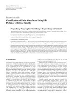
Figure 2: RMS voltage values versus time (shadowed parts: transition segments). (a)–(f): (a) an interruption due to fault; (b) nonfault
interruption; (c) induction motor starting; (d) transformer saturation; (e) step change; and (f) single stage voltage dip due to fault.
(3) Detecting the boundaries of segments
A simple step is used to detect the boundaries of segments
under two hypotheses:
H

0
(event-segment) : M
RMS


t
k

<δ,
H
1
(transition-segment) : M
RMS


t
k

≥
δ,
(7)
where δ is a threshold. A transition segment starts at the first

t
k
for which H
1
is satisfied, and ends at the first

t

k
for which
M
RMS
(

t
k
) <δoccurs after a t ransition segment is detected.
It is recommended to use waveform data for feature ex-
traction whenever available, as extracting features from the
RMS voltages leads to loss of information. It is however pos-
sible, as shown in [20], to perform segmentation based on
Math H. J. Bol len et al. 5
0 200 400 600 800 1000
1
0.5
0
0.5
1
Time (ms)
Voltage ( pu)
(a)
0 200 400 600 800 1000
0.6
0.8
1
Time (ms)
Magnitude (pu)
(b)

0 200 400 600 800 1000
0
25
50
Time (ms)
Detection index
(c)
Figure 3: Using the Kalman filter to detect sudden changes (N =
20): (a) original voltage waveforms from 3 phases; (b) the detected
transition points (marked on the fundamental voltages) that are
used as the boundaries of segmented blocks; (c) the detection in-
dex by considering all three phases.
recorded RMS sequences. The performance of the resulting
classifier is obviously less than that for a classifier based on
the full waveform data.
3. UNDERSTANDING POWER QUALITY
DISTURBANCES: UNDERLYING CAUSES
AND THEIR CHARACTERIZATION
Characterizing the underlying causes of power quality distur-
bances and extrac ting relevant features based on the recorded
voltagesorcurrentsisingeneraladifficult issue: it requires
understanding the problems and phenomena of power qual-
ity disturbances using power system knowledge. A common
and essential step for successfully applying signal processing
techniques towards any particular type of signals is largely
dependent on understanding the nature of that signal (e.g.,
speech, radar, medical signals) and then “translating” them
into the problems from signal processing viewpoints. This
section, through examples, contributes to understanding and
“translating” several types of power quality disturbances into

the perspective of signal processing. With visual inspection
of the waveform or the spectra of disturbances, the suc-
cess rate is very much dependent on a person’s understand-
0 20 40 60 80 100 120 140 160 180 200 220
1
0.5
0
0.5
1
Time (ms)
Voltage ( pu)
(a)
0 20 40 60 80 100 120 140 160 180 200 220
0.9
0.95
1
Time (ms)
Voltage
magnitude (pu)
(b)
Figure 4: Induction motor starting: (a) voltage waveforms; (b) volt-
age magnitude (measurement in a 400 V network).
ing and previous knowledge of disturbances in power sys-
tems. An automatic classification system should be based at
least in part on this human expert knowledge. The inten-
sion is to give some examples of voltage disturbances that are
caused by different types of underlying reasons. One should
be aware that this list is by far complete. It should further
be noted that the RMS voltage as a function of time (or,
RMS voltage shape) is used here to present the events, even

though the features may be better extracted from the ac-
tual waveforms or from some other transform domain. We
will emphasize that RMS sequences are by far the only time-
dependent characteristics to describe the disturbances; many
other characteristics can also be exploited [5].
Induction motor starting
The voltage waveform and RMS voltages for a dip due to in-
duction motor starting are shown in Figure 4. A sharp volt-
age drop, corresponding to the energizing of the motor, is
followed by gradual voltage recovery when the motor cur-
rent decreases towards the normal operating current. As an
induction motor takes the same current in the three phases,
the voltage drop is the same in the three phases.
Transformer energizing
The energizing of a transformer gives a large current, related
to the saturation of the core flux, which results in a voltage
dip. An example is shown in Figure 5, where one can observe
that there is a sharp voltage drop followed by gradual voltage
recovery. As the saturation is different in the three phases, so
is the current. The result is an unbalance voltage dip; that is, a
dip with different voltage magnitude in the three phases. The
dip is further associated with a high harmonic distortion,
including even harmonics.
6 EURASIP Journal on Advances in Signal Processing
0 50 100 150 200 250 300
1
0.5
0
0.5
1

Time (ms)
Voltage ( pu)
(a)
0 50 100 150 200 250 300
0.7
0.8
0.9
1
1.1
Time (ms)
Voltage
magnitude (pu)
(b)
Figure 5: Voltage dip due to transformer energizing: (a) voltage
waveforms; (b) voltage magnitude (EMTP simulation).
0 20 40 60 80 100 120 140 160 180 200
1
0.5
0
0.5
1
Time (ms)
Voltage ( pu)
(a)
0 20 40 60 80 100 120 140 160 180 200
0.85
0.9
0.95
1
1.05

Time (ms)
Voltage
magnitude (pu)
(b)
Figure 6: Voltage disturbance due to load switching: step change
measurement: (a) voltage waveforms; (b) voltage magnitude (mea-
surement in an 11 kV network).
Load switching
The switching of large loads gives a drop in voltage, but with-
out the recovery after a few seconds, see Figure 6. The equal
drop in the three phases indicates that this event was due to
the sw itching of a three-phase load. The disconnection of the
load will give a similar step in voltage, but in the other direc-
tion.
Capacitor energizing
Capacitor energizing gives a rise in voltage as shown in
Figure 7, associated with a transient, in this example a minor
0 20 40 60 80 100 120 140 160 180 200
1
0.5
0
0.5
1
Time (ms)
Voltage ( pu)
(a)
0 20 40 60 80 100 120 140 160 180 200
0.98
1
1.02

1.04
1.06
1.08
Time (ms)
Voltage
magnitude (pu)
(b)
Figure 7: Voltage disturbance due to capacitor energizing: (a) volt-
age waveforms; (b) voltage magnitude (measurement in a 10 kV
network).
transient, and often a change in harmonic spectrum. Capac-
itor banks in the public grid are always three phase so that
the same voltage rise will be observed in the three phases.
The recording shown here is due to synchronized capaci-
tor energizing where the resulting transient is small. Non-
synchronized switching gives severe tra nsients which can be
usedasafeaturetoidentifythistypeofevent.Severaltypes
of loads are equipped with a capacitor, for example, as part
of their EMI-filter. The event due to switching of these loads
will show similar characteristics to capacitor energizing. Ca-
pacitor de-energizing will g ive a drop in voltage in most cases
without any noticeable transient.
Voltage dip due to a three-phase fault
The most common cause of severe voltage dips in distri-
bution and transmission systems are symmetrical and non-
symmetrical faults. The large fault current gives a drop in
voltage between fault initiation and the clearing of the fault
by the protection. An example of a voltage dip due to a sym-
metrical (three-phase) fault is shown in Figure 8: there is a
sharp drop in voltage (corresponding to fault initiation) fol-

lowed by a period with constant voltage and a sharp recov-
ery (corresponding to fault clearing). The change in voltage
magnitude has a rectangular shape. Further, all three phases
are affected in the same way for a three-phase fault.
Voltage dip due to an asymmetric fault
Figure 9 shows a voltage dip due to an asymmetric fault (a
fault in which only one or two phases are involved). The dip
in the individual phases is the same as for the three-phase
fault, but the drop in voltage is different in the three phases.
Math H. J. Bol len et al. 7
0 50 100 150 200 250 300 350
1
0.5
0
0.5
1
Time (ms)
Voltage ( pu)
(a)
0 50 100 150 200 250 300 350
0.2
0.4
0.6
0.8
1
1.2
Time (ms)
Voltage
magnitude (pu)
(b)

Figure 8: Voltage dip due to a symmetrical fault: (a) voltage wave-
forms; (b) voltage magnitude (measurement in an 11 kV network).
0 100 200 300 400
1
0.5
0
0.5
1
Time (ms)
Voltage ( pu)
(a)
0 100 200 300 400
0.5
0.6
0.7
0.8
0.9
1
1.1
Time (ms)
Voltage
magnitude (pu)
(b)
Figure 9: Voltage dip due to an asymmetrical fault: (a) voltage
waveforms; (b) voltage magnitude (measurement in an 11 kV net-
work).
Self-extinguishing fault
Figure 10 shows the waveform and RMS voltage due to
a self-extinguishing fault in an impedance-earthed system.
The fault extinguishes almost immediately, giving a low-

frequency (about 50 Hz) oscillation in the zero-sequence
voltage. This oscillation gives the overvoltage in two of the
three-phase voltages. This event is an example where the cus-
tomers are not affected, but information about its occur-
rence and cause is still of importance to the network oper-
ator.
0 20 40 60 80 100 120 140
1
0.5
0
0.5
1
Time (ms)
Voltage ( pu)
(a)
0 20 40 60 80 100 120 140
0.7
0.8
0.9
1
1.1
1.2
1.3
Time (ms)
Voltage
magnitude (pu)
(b)
Figure 10: A self-extinguishing fault: (a) voltage waveforms; (b)
voltage magnitude (measurement in a 10 kV network).
0 100 200 300

1.5
1
0.5
0
0.5
1
1.5
Time (ms)
Voltage ( pu)
(a)
0 100 200 300
0.6
0.8
1
1.2
1.4
Time (ms)
Voltage
magnitude (pu)
(b)
Figure 11: Overvoltage swell due to a fault: (a) voltage waveforms;
(b) voltage magnitude (measurement in an 11 kV network).
Voltage swell due to earthfault
Earthfaults in nonsolidly-earthed systems result in overvolt-
ages in two or three phases. An example of such an event
is shown in Figure 11. In this case, the voltage rises in one
phase, drops in another phase, and stays about the same in
the third phase. This measurement was obtained in a low-
resistance-earthed system where the fault current is a few
times the nominal current. In systems with lower fault cur-

rents, typically both nonfaulted phases show an increase in
voltage magnitude.
8 EURASIP Journal on Advances in Signal Processing
0 100 200 300 400 500
1
0.5
0
0.5
1
Time (ms)
Voltage ( pu)
(a)
0 100 200 300 400 500
0.6
0.7
0.8
0.9
1
1.1
Time (ms)
Voltage
magnitude (pu)
(b)
Figure 12: Voltage dip due to fault, with the influence of induc-
tion motor load during a fault: (a) voltage waveforms; (b) voltage
magnitude (measurement in an 11 kV network).
Induction motor influence during a fault
Induction motors are affected by the voltage drop due to a
fault. The decrease in voltage leads to a drop in torque and
adropinspeedwhichinturngivesanincreaseincurrent

taken by the motor. In the voltage recording, this is visible
as a slow decrease in the voltage magnitude. An example is
shown in Figure 12: a three-phase fault with motor influence
during and after the fault.
4. RULE-BASED SYSTEMS FOR CLASSIFICATION
4.1. Expert systems
A straightforward way to implement knowledge from power-
quality experts in an automatic classification system is to de-
velop a set of classification rules and implement these rules
in an expert system. Such systems are proposed, for example,
in [6, 7, 14, 19, 20].
This section is intended to describe expert systems
through examples of some basic building blocks and rules
upon which a sample system can be built. It is worth men-
tioning that the sample expert system described in this sec-
tion is designed to only deal with a certain number of distur-
bance types rather than all types of disturbances. For exam-
ple, arcing faults and harmonic/interharmonic disturbances
are not included in this system, and will therefore be classi-
fied as unknown/rejected type by the system.
A typical rule-based expert system, shown in the block
diagram of Figure 13, may consist of the following blocks.
(i) User interface
It is the interface where the data are fed as the input into a
system (e.g., from the output of a power system monitor),
User
interface
Explanation
system
Inference

engine
Knowledge
base editor
Case-specific
data
Knowledge
base
Figure 13: Block diagram of an expert system.
the classification or diagnostic results are the output through
the interface (e.g., a computer terminal).
(ii) Inference engine
An inference engine performs the reasoning with the expert
system knowledge (or, rules) and the data from a particular
problem.
(iii) Explanation s ystem
An explanation system allows the system to explain the rea-
soning to a user.
(iv) Knowledge-base editor
The system may sometimes include this block so as to allow
a human expert to update or check the rules.
(v) Knowledge base
It contains all the rules, usually a set of IF-THEN rules.
(vi) Case-specific data
This block includes data provided by the user and can also
include partial conclusions or additional information from
the measurements.
4.2. Examples of rules
The heart of the expert system consists of a set of rules,
where the “real intelligence” by human experts is translated
into “artificial intelligence” for computers. Some example of

rules, using RMS sequences as input, are given below. Most
of these rules can be deducted from the description of the
different events given in the previous section.
Rule 1 (interruption). IF at least two consecutive RMS volt-
ages are less than 0.01 pu, THEN the event is an interruption.
Rule 2 (voltage swell). IF at least two consecutive RMS volt-
ages are more than 1.10 pu, AND the RMS voltage drops be-
low 1.10 pu within 1 minute, THEN the event is a voltage
swell.
Math H. J. Bol len et al. 9
Rule 3 (sustained overvoltage). IF the RMS voltage remains
above1.06pufor1minuteorlonger,ANDtheeventisnota
voltage swell, THEN the event is a sustained overvoltage.
Rule 4 (voltage dip). IF at least two consecutive RMS volt-
ages are less than 0.90 pu, AND the RMS voltage rises above
0.90 pu within 1 minute, AND the event is not an interrup-
tion, THEN the event is a voltage dip.
Rule 5 (sustained undervoltage). IF the RMS voltage remains
below 0.94 pu for 1 minute or longer, AND the event is not a
voltage dip, AND the event is not an interru ption, THEN the
event is a sustained undervoltage.
Rule 6 (voltage step). IF the RMS voltage remains between
0.90 pu and 1.10 pu and the difference between two consec-
utive RMS voltages remains within 0.0025 pu of its average
value for at least 20 seconds before and a fter the step, and the
event is not a sustained overvoltage, AND the event is not a
sustained undervoltage, THEN the event is a voltage step.
Note that these rules do allow for an event being both
a voltage swell and a voltage dip. There are also events that
possibly do not fall in any of the event classes. The inference

engine should b e such that both combined events and non-
classifiable events are recognized. Alternatively, two addi-
tional e vent classes may be defined as “combined dip-swell”
and “other events.” For further classifying the underlying
causes of a voltage dip, the following rules may be applied.
Rule 7 (voltage dip due to fault). IF the RMS sequence has
a fast recovery after a dip (rectangular shaped recovery),
THEN the dip is due to a fault (rectangular shaped is caused
by protection operation).
Rule 8 (induction motor starting). IF the RMS sequences for
all three phases of voltage recover gradually but with approx-
imately the same voltage drop, THEN it is caused by induc-
tion motor starting.
Rule 9 (transformer saturation). IF the RMS sequences for
all three phases of voltage recover gradually but with different
voltage drop, THEN it is caused by transformer saturation.
4.3. Application of an expert system
A similar set of rules, but using waveform data as input, has
been implemented in an exper t system and applied to a large
number of disturbances (however, limited to 9 types), ob-
tained in a medium-voltage distribution system [19, 20].
The expert system is designed to classify each voltage dis-
turbance into one of the 9 classes, according to its underly-
ing cause. The list of underlying causes of disturbances being
considered in this expert system includes
(i) energizing,
(ii) nonfault interruption,
(iii) fault interruption,
(iv) transformer saturation due to fault,
(v) induction motor starting,

Rectangular
voltage dips
Nonrectangular
voltage dips
Step changes
in voltage
Faults
Duration less
than 3 cycles
Single stage
Multistage
Transformer
saturation
Induction motor
starting
Interruption
Energizing
Load switching
Voltage compensation
Self-extinguishing
fault
Fuse-cleared fault
Change in the fault
Change in the system
Normal switching
Due to reclosing
Normal operation
Due to fault
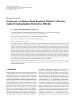
Figure 14: A tree structured inference process for classifying power
system disturbance recordings.

(vi) step change,
(vii) transformer saturation followed by protection opera-
tion,
(viii) single stage dip due to fault,
(x) Multistage dip due to fault.
Some further analysis and classification are then applied, for
example,
(i) seven types of dip (type A, Ca, Cb, Cc, Da, Db, Dc, as
defined in [3]);
(ii) step change associated with voltage increase/decrease;
(iii) overvoltage associated with energizing/transformer
saturation/step change/faults;
(iv) fault related to starting/voltage swell/clearing.
The tree-structured inference process for classifying the
underlying causes is shown in Figure 14.
Table 1 shows the results from the expert system. Com-
paring with the ground truth (manually classified results
from power system experts), the expert system has achieved
approximately 97% of classification rate for a total of 962 dis-
turbance recordings.
5. STATISTICAL LEARNING AND CLASSIFICATION
USING SUPPORT VECTOR MACHINES
5.1. Motivations
A natural question arises before we describe SVM classifiers.
Why should one be interested in an SVM when there are
many other classification methods? Two main issues of inter-
est in SVM classifiers are the generalization performance and
the complex ity of classifier which is a practical implementa-
tion concern.
When designing a classification system, it is natural that

one would like the classifier to have a good generalization per-
formance (i.e., the performance on the test set rather than on
10 EURASIP Journal on Advances in Signal Processing
Table 1: Classification results for 962 measurements.
Type of events
Number of classified
events
Energizing 104
Interruption
(by faults/nonfaults)
13 88
Transformer saturation
(normal/protection operation)
119 6
Step change
(increase/decrease)
15 21
Fault-dip (single stage) 455
Fault-dip (multistage)
(fault/system change)
56 56
Other nonclassified
(short duration/overvoltage)
16 13
the training set). If one uses too many training samples, a
classifier might be overfitted to the training samples. How-
ever, if one has too few training samples, one may not be able
to obtain a sufficient statistical coverage to most possible sit-
uations. Both cases will lead to poor performance on the test
data set. For an SVM classifier, there is a guarantee of the up-

per error bound on the test set based on statistical learning
theory. Complexity of classifiers is a practical implementa-
tion issue. For example, a classifier, for example, a Bayesian
classifier, may be elegant in theory, however, a high compu-
tational cost may hinder its practical use. For an SVM, the
complexity of the classifier is associated with the so-called
VC dimension.
An SVM classifier minimizes the generalization error on
the test set under the structural risk minimization (SRM)
principle.
5.2. SVMs and the generalization error
One special characteristic of an SVM is that instead of di-
mension reduction is commonly employed in pattern clas-
sification systems, the input space is nonlinearly mapped by
Φ(
·) onto a high-dimensional feature space, where Φ(·)is
a kernel satisfying Mercer’s condition. As a result of this,
classes are more likely to be linearly separable in the high-
dimensional space rather than in a low-dimensional space.
Let input training data and the output class labels be de-
scribed as pairs (x
i
, d
i
), i = 1, 2, , N, x
i
∈ R
m
0
(i.e., m

0
di-
mensional input space) and d
i
∈ Y (i.e., the decision space).
As depicted in Figure 15, the spaces and the mappings for
an SVM, a nonlinear mapping function Φ(
·)isfirstapplied
which maps the input-space
R
m
0
onto a high-dimensional
feature-space F ,
Φ :
R
m
0
−→ F x
i
−→ Φ

x
i

,(8)
where Φ is a nonlinear mapping function associated with a
kernel function.
x
x

x
x
x
x
x
o
o
o
o
o
o
o
o
Φ(x)
Φ(x)
Φ(x)
Φ(x) Φ(x)
Φ(x)
Φ(x)
Φ(o) Φ(o)
Φ(o)
Φ(o)
Φ(o)
Φ(o)
Φ(o)
Φ(o)
C
1
C
2

R
m
0
F Y
Φ(
) f ( )
Input space Feature space Decision space
Figure 15: Different spaces and mappings in a support vector ma-
chine.
Then, another function f (·) ∈ F is applied to map the
high-dimensional feature space F onto a decision space,
f : F
−→ Y Φ

x
i

−→
f

Φ

x
i

. (9)
The best function f (
·) ∈ F that may correctly classify a un-
seen example (x, d) from a test set is the one minimizing the
expected error, or the generalization error,

R( f )
=

l

f

Φ(x)

, d

dP

Φ(x), d

, (10)
where l(
·) is the loss function, and P(Φ(x), d) is the proba-
bility of (Φ(x), d) which can be obtained if the probability of
generating the input-output pair (x, d) is known. A loss (or,
error) is occurred if f (Φ(x))
= d.
Since P(x, d) is unknown, we cannot directly minimize
(10). Instead, we try to estimate the function f (
·) that is close
to the optimal one from the function class
F using the t rain-
ing set. It is worth noting that there exist many f (
·) that give
perfect classification on the training set; however they give

different results on the test set.
According to VC theory [26–29], we choose a function
f (
·) that fits to the necessary and sufficient conditions for
the consistency of empirical risk minimization,
lim
n→∞
P

sup
f

R( f ) − R
emp
( f )

>ε

=
0, ∀ε>0, (11)
where the empirical risk (or the training error) is defined on
the training set
R
emp
( f ) =
1
N
N

i=1

l

f

Φ

x
i

, d
i

(12)
and N is the total number of samples (or feature vectors) in
the training set. A specific way to control the complexity of
function class
F is given by VC theory and the structural risk
minimization (SRM) principle [27, 30]. Under the SRM prin-
ciple, the function class
F (and the function f ) is chosen such
that the upper bound of the generalization error in (10)is
minimized. For all δ>0and f
∈ F, it follows that the bound
of the generalization error
R( f )
≤ R
emp
( f )+

h


ln(2N/h)+1

−
ln(δ/4)
N
(13)
Math H. J. Bol len et al. 11
holds with a probability of at least (1 − δ)forN>h,whereh
is the VC dimension for the function class
F. The VC dimen-
sion, roughly speaking, measures the maximum number of
training samples that can be correctly separated by the class
of functions
F.Forexample,N data samples can be labeled to
2
N
possible ways in a binary class Y ={1, −1} case, of which
there exists at least one set of h samples that can be correctly
classified to their class labels by the chosen function class
F.
Asonecanseefrom(13), minimization of R( f )isob-
tained by yielding a small training error R
emp
( f ) (the 1st
term) while keeping the func tion class as small as possible
(the 2nd term). Hence, SVM learning can be viewed as seek-
ing the best function f (
·) from the possible function set F
according to the SRM principle which gives the lowest upper

bound in (13).
Choosing a nonlinear mapping function Φ in (8)isas-
sociated with selecting a kernel function. Kernel functions in
an SVM must satisfy Mercer’s condition [28]. Roughly speak-
ing, Mercer’s condition states for which kernel k(x
i
, x
j
) there
exists (or does not exist) a pair
{F , Φ}. Or, whether a kernel
is a dot product in some feature space F . Choosing different
kernels leads to different types of SVMs. The significance of
using kernel in SVMs is that, instead of solving the primal
problem in the feature space, one can solve the dual problem
in SVM learning which only requires the inner products of
feature vectors rather than features themselves.
5.3. Soft-margin SVMs for linearly
nonseparable classes
Consider a soft-margin SVM for linearly nonseparable class-
es. The strategy is to allow some training error R
emp
( f ) in the
classifier in order to achieve less error on the test set, hence
(13) is minimized. This is because zero training error can
lead to overfitting and may not minimize the error on the
test set.
An important concept in SVMs is the margin.Amargin
of a classifier is defined as the shortest distance between the
separating boundary and a n input tra ining vector that can

be correctly classified (e.g., classified as being d
1
= +1 and
d
2
=−1). Roughly speaking, optimal solution to an SVM
classifier is associated with finding the maximum margin.
For a soft-margin SVM, support vectors can lie on the mar-
gins as well as inside the margins. Those support vectors that
lie in between the separating boundaries and the margins
represent misclassified samples from the training set.
Let prelabeled training sample pairs b e (x
1
, d
1
), ,
(x
N
, d
N
), where x
i
are the input vectors and d
i
are the cor-
responding labels in a binary class Y
={−1, +1}. A soft-
margin SVM is described by a set of equations:
d
i


w, Φ

x
i

+ b

≥
1 − ξ
i
, ξ
i
≥ 0, i = 1, 2, , N,
(14)
or as a quadratic optimization problem:
min
w,b,ξ

1
2
w
2
+ C
N

i=1
ξ
i


, (15)
where C
≥ 0 is a user-specified regularization parameter
that determines the trade-off between the upper bound on
the complexity term and the empirical error (or, training
error), and ξ
i
are the slack variables. C can be determined
empirically, for example, though a cross-validation process.
This leads to the primal form of the Lagrangian optimization
problem for a soft-margin SVM,
L(w, b, α, ξ, μ)
=
1
2
w
2
+ C
N

i=1
ξ
i
−
N

i=1
μ
i
ξ

i
−
N

i=1
α
i

d
i

w, Φ

x
i

+ b

−
1+ξ
i

,
(16)
where μ
i
is the Lagrange multiplier to enforce the positivity
of ξ
i
. Solutions to the soft-margin SVM can be obtained by

solving the dual problem of (16),
max
α

N

i=1
α
i
−
1
2
N

i, j=1
α
i
α
j
d
i
d
j
k

x
i
, x
j



subject to
N

i=1
α
i
d
i
= 0, C ≥ α
i
≥ 0, i = 1, 2, , N.
(17)
The KKT (Karush-Kuhn-Tucker) conditions for the pri-
mal optimization problem [ 31]are
α
i

d
i

w, Φ

x
i

+b

−
1+ξ

i

=
0, μ
i
ξ
i
=0, i=1,2, , N.
(18)
The KKT conditions are associated with the necessary and
in some cases sufficient conditions for a set of variables to
be optimal. The Lagrangian multipliers α
i
are nonzero only
when the KKT conditions are met.
The corresponding vectors x
i
, for nonzero α
i
, satisfying
the 1st s et of equations in (18) are the so-called support vec-
tors.Onceα
i
are determined, the optimal solution w can be
obtained as
w
=
N
s


i=1
α
i
d
i
Φ

x
i

, (19)
where x
i
∈ SV, and the bias b can be determined by the KKT
conditions in (18).
Instead of solving the primal problem in (16), one usu-
ally solve the equivalent dual problem of a soft-margin SVM
described as
max
α

N

i=1
α
i
−
1
2
N


i, j=1
α
i
α
j
d
i
d
j
k

x
i
, x
j


subject to
N

i=1
α
i
d
i
= 0, C ≥ α
i
≥ 0, i = 1, 2, , N
(20)

noting that the slack variables ξ
i
and the weight vector w do
not appear in the dual form. Finally, the decision function
12 EURASIP Journal on Advances in Signal Processing
x
1
x
2
x
N
s
.
.
.
.
.
.
.
.
.
Test dat a
x
k(x
1
, x)
k(x
2
, x)
k(x

N
s
, x)
α
1
d
1
α
2
d
2
α
N
s
d
N
s
Bias b
+
Support vectors
from training set
Kernels
Classification
sgn


i
α
i
d

i
k(x
i
, x)+b

Figure 16: Block diagram of an SVM classifier for a two-class case.
for a soft-margin SVM classifier is
f (x)
= sgn

N
s

i=1
α
i
d
i
k

x, x
i

+ b

, (21)
where N
s
is the number of support vectors x
i

, x
i
∈ SV, and
k(x, x
i
) =Φ(x), Φ(x
i
) is the selected kernel function. So-
lution to (20)canbeobtainedasa(convex)quadraticpro-
gramming (QP) problem [32]. Figure 16 shows the block di-
agram of an SVM classifier where x is the input vector drawn
from the test set, and x
i
, i = 1, , N
s
, are the support vec-
tors drawn from the t raining set. It is worth noting that al-
though the block diagram structure of the SVM looks similar
to an RBF neur a l network, the fundamental differences exist.
First, the weights α
i
d
i
to the output of an SVM contain La-
grange multipliers α
i
that are associated with the solutions of
the constrained optimization problem in the SVM learning,
such that the generalization error (or the classification error
on the test set) is minimized. In RBF neural networks, the

weights are selected for minimizing the empirical error (i.e.,
the error between the desired outputs d and the network out-
puts from the training set). Second, for a general multilayer
neural network, activation functions are used in the hidden
layer to a chieve the nonlinearity, while an SVM employs a
kernel function k(
·) only dependent on the difference of x
from the test set and the support vectors from the training
set.
5.4. Radial basis function kernel C-SVMs for
classification of power disturbances
The proposed SVMs use Gaussian RBF (radial-basis func-
tion) kernels, that is,
k(x, y)
= exp

−
x − y
2
γ

. (22)
For a C-SVM with RBF kernels, there are two parameters to
be selected: one is the regularization parameter C in (16), an-
Table 2: AND problem for classifying voltage dips due to faults.
Input vector x Desired response d
(1,1) +1
(1,0)
−1
(0,0)

−1
(0,1)
−1
other is the kernel parameter γ. An RBF kernel is chosen since
it can behave like a linear kernel or a sigmoid kernel under
different parameter settings. An RBF is also known to have
less numerical difficulties since the kernel matrix K
= [k
ij
],
i, j
= 1, , N, is symmetric positive definite. The parameters
(C, γ) should be determined prior to the training process.
Cross validation is used for the purpose of finding the best
parameters (C, γ). We use the simple grid-search method de-
scribed in [33]. First, a coarse grid-search is applied, for ex-
ample, C
={2
−5
,2
−3
, ,2
15
}, γ ={2
15
,2
13
, ,2
−3
}.The

search is then tuned to a finer grid in the region where the
predicted error rate from the cross validation is the lowest
in the coarse search. Once (C, γ) are determined, the whole
training set is used for the training. The learned SVM with
fixed weights is then ready to be used as a classifier for sam-
ples x drawn from the test set. Figure 17 describes the block
diagram of the entire process.
It is worth mentioning that normalization is applied be-
fore each feature vector before it is fed into the classifier ei-
ther for training or classification. Normalization is applied
to each component (or subgroup of components) in a fea-
ture vector, so that a ll components have the same mean and
variance. Noting that the same normalization process should
be applied to the training and test sets.
5.5. Example 1
To show how an SVM can be used for classification of power
system disturbances, a very simple hypothetical example is
described of classify ing fault-induced voltage dips.
A voltage dip is defined as an event during which the volt-
age drops below a certain level (e.g., 90% of nominal). Fur-
thermore, for dips caused by faults, RMS voltage versus time
is close to a rectangular shape. However, a sharp drop fol-
lowed by a slow recovery is c aused by transformer saturation
or induction motor starting depending on whether they have
a similar voltage dropping in all three phases.
In the ideal case, classification of fault-induced voltage
dips can be descr ibed as an AND problem. Let each fea-
ture vector x
= [x
1

, x
2
]
T
consist of two components, where
x
1
∈{0, 1} indicates whether there is a fast drop in RMS volt-
age to below 0.9 pu (i.e., rectangular shaped drop). If there
is a sharp voltage drop to below 0.9 pu, then x
1
is set to 1.
x
2
∈{0, 1} indicates whether there is a quick recovery in
RMS voltage (i.e., rectangular shaped recovery in the RMS
sequence). When the recovery is fast, then x
2
is set to 1.
Also, define the desired output for dips due to faults as
d
= 1, and d =−1 for all other dips. Tab le 2 describes such
an AND operation.
Math H. J. Bol len et al. 13
x
i
from
the training set
x from
the test set

Scaling and
normalization
Scaling and
normalization
K-fold cross validation
(training + prediction)
Best (C
, γ )
Training
(for the entire set)
Learned SVM
classifier
Class
labels
Figure 17: Block diagram for learning an RBF kernel SVM. The SVM is subsequently used as a classifier for input x from a test set.
However, a voltage drop or recovery will never be abso-
lutely instantaneous, but instead always take a finite time.
The closeness to rectangularity is a fuzzy quantity that can be
defined as a continuous function ranging between 0 and 1.0
(e.g., by defining a fuzzy function, see [34]), where 0 implies
a complete flat shape while 1.0 an ideal rectangular shape
(θ
= 90

). Consequently, each component of the feature vec-
tor x takes a real value within [0, 1].
In this simple example, the training set contains the fol-
lowing 12 vectors:
x
1

= (1.0, 1.0), x
2
= (1.0, 0.0), x
3
= (0.0, 0.0),
x
4
= (0.0, 1.0), x
5
= (0.8, 0.7), x
6
= (0.9, 0.4),
x
7
= (0.2, 0.8), x
8
= (0.4, 0.8), x
9
= (0.8, 0.9),
x
10
= (0.9, 0.5), x
11
= (0.3, 0.2), x
12
= (0.3, 0),
(23)
and their corresponding desired o utputs are
d
1

= d
5
= d
9
= +1,
d
2
= d
3
= d
4
= d
6
= d
7
= d
8
= d
10
= d
11
= d
12
=−1.
(24)
Figure 18 shows the decision boundaries obtained from
training an SVM using Gaussian RBF kernels with two dif-
ferent γ values (related to the spread of kernels). One can see
that the bending of the decision boundary (i.e., the solid line)
changes depending on the choice of the par a meter related

to Gaussian spread. In Figure 18(a), the RBF kernels have a
relatively large spread and the decision boundary becomes
very smooth which is close to a linear boundary. While in
Figure 18(b) the RBFs have a smaller spread and the decision
boundary has a relatively large bending (nonlinear bound-
ary). If the features of event classes are linearly nonseparable,
a smoother boundary would introduce more training errors.
Interestingly enough, the decision boundary obtained from
the training set (containing feature vectors with soft values of
rectangularity in voltage drop and recovery) divides the fea-
ture space into two regions where the up-right region (notice
that the shape of region makes good sense!) is associated with
the fault-induced dip events.
When the training set contains more samples, one may
expect an improved classifier. Using more training data will
lead to changes in the decision boundary, the margins, and
the distance between the margins and the boundary. We
might also find some support vectors that are lying between
the boundary and the margin, indicating training errors.
However, for achieving a good performance on the test set,
some training errors have to be allowed.
It is worth mentioning that, to apply this example in real
applications, one should first compute the RMS sequence
from a given power quality disturbance recording, followed
by extracting these features from the shape of RMS sequence.
Further, using features instead of directly using signal wave-
form for classification is a common practice in pattern classi-
fication systems. Advantages of using features instead of sig-
nal waveform include, for example, reducing the complexity
of classification systems, exploiting the characteristics that

are not obvious in the waveform (e.g., frequency compo-
nents), and using distur bance sequences without time warp-
ing.
5.6. Example 2
A more realistic classifier has been developed to distinguish
between five different types of dips. The classifier has been
trained and tested using features extracted from the measure-
ment data obtained from two different networks.
The following five classes of disturbances are distin-
guished (see Table 3):
(D1) voltage dips with a main drop in one phase;
(D2) voltage dips with a main, identical, drop in two phases;
(D3) voltage dips due to three phase faults;
(D4) voltage dips with a main, but different, drop in two
phases;
(D5) voltage disturbances due to transformer energizing.
Each measurement recording includes a short prefault
waveform (approximately 2 cycles long) followed by the
waveform containing a disturbance. The nominal frequency
of the power networks is 50 Hz and the sampling frequencies
are 1000 Hz, 2000 Hz, or 4800 Hz. The data were originated
from two different networks from two European countries A
and B.
Synthetic data have been generated by using the power
network simulation toolbox “SimPowerSystems” in Matlab.
The model is a 11-kV network consisting of a voltage source,
an incoming line feeding four outgoing lines via a busbar.
The outgoing lines are connected to loads with different load
characteristics in terms of active and reactive power. At one of
these lines, faults are generated. In order to simulate different

14 EURASIP Journal on Advances in Signal Processing
012345678910
0
1
2
3
4
5
6
7
8
9
10 1
2
3
4
5
6
7
8
9
10
11
12
(a)
012345678910
0
1
2
3

4
5
6
7
8
9
10 1
2
3
4
5
6
7
8
9
10
11
12
(b)
Figure 18: The decision boundaries and support vectors obtained
by training an SVM with Gaussian RBF kernel functions. Solid line:
the decision boundary; dashed lines: the margins. (a) The parame-
ter for RBF kernels is γ
= 36m
0
; (b) the parameter for RBF kernels
is γ
= 8m
0
. For both cases, the regularization parameter is C = 10,

and m
0
= 2 is the size of the input vector. Solid line is the deci-
sion boundary. Support vectors are the training vectors that are lo-
cated on the margins (the dotted lines) and in between the bound-
ary and the margin (misclassified samples). For the given training
set, there is no misclassified samples. The two sets of feature vectors
are marked with rectangular and circles, respectively. Notice that
only support vectors are contributed to the location of the decision
boundary and margins. In the figure, all feature values are scaled by
a factor of 10.
Table 3: Number of voltage recordings used.
Disturbance type Network A Network B From synthetic
D1 141 471 225
D2
181 125 225
D3
251 14 223
D4
127 196 250
D5
214 0 0
waveforms, the lengths of the incoming line and the outgoing
lines as well as the duration of the disturbances are randomly
varied within given limits. Finally, the voltage disturbances
are measured at the busbar.
Table 4: Classification results using training and test data from net-
work A.
D1 D2 D3 D4 D5 Nonclassified
Detection

rate
D1 630130 4 88.7%
D2
0 84 4 0 0 3 92.3%
D3
5 3 113 0 0 5 89.7%
D4
0 0 0 63 1 0 98.4%
D5
0 0 0 0 103 4 96.3%
Table 5: Classification results for data f rom network B, where the
SVM is trained with data from network A.
D1 D2 D3 D4 Nonclassified
Detection
rate
D1 463 1 0 1 6 99.1%
D2
0 118 0 0 7 94.4%
D3
2 1 11 0 0 78.6%
D4
0 1 0 187 8 95.4%
Segmentation is first applied to each measurement
recording. Data in the event segment after the first transition
segment are used for extracting features. The features are
based on RMS shape and the harmonic energy. For each
phase, the RMS voltage versus time is computed. Twenty
feature components are extracted from equally distance-
sampling the RMS sequence, starting from the triggering
point of the disturbance. Further, to include possible dif-

ferences of harmonic distributions in the selected classes of
disturbances, some harmonic-related features are also used.
Four harmonic-related feature components are extracted
from the magnitude spectrum from the data in the event seg-
ment. They are the magnitudes of 2nd, 5th, and 9th harm on-
ics and the total harmonics distortion (THD) with respect to
the magnitude of power system fundamental frequency com-
ponent. Therefore, for each three-phase recording, the fea-
ture vector consists of 72 components. Feature normalization
is then applied to ensure that all components are equally im-
portant. It is worth mentioning that since there are 60 feature
components related to the 3 RMS sequences and 12 feature
components related to harmonic distortions, it implies that
more weight has been put on the shape of RMS voltage as
compared to harmonic distortion.
C-SVM with RBF kernels is chosen. Grid search and a
3-fold validation are used for determining the optimal pa-
rameters (C, γ) for the SVM. Further, we use separate SVMs
for5different classes, each classifying between one particu-
lar type and the remaining. These SVMs are connected in a
binary tree structure.
Experiment results
Case 1. For the first case, data from the network A are split
into two subsets, one is used for training, and the other is
Math H. J. Bol len et al. 15
Table 6: Classification results for data from network A, where the
SVM is trained with data from network B.
D1 D2 D3 D4 Nonclassified
Detection
rate

D1 137 0 2 1 1 97.2%
D2
0 154 16 0 11 85.1%
D3
10 1 232 0 8 92.4%
D4
4 1 1 121 0 95.2%
Table 7: Classification results for data f rom network B, where the
SVM is trained with data from network A and synthetic data.
D1 D2 D3 D4 Nonclassified
Detection
rate
D1 473 1 0 0 1 99.5%
D2
0 122 2 0 1 97.6%
D3
0 0 187 0 9 95.4%
D4
15 31 0 14 7 20.0%
used for testing. The resulting classification results are shown
in Table 4. The resulting overall detection rate is 92.8% show-
ing the ability of the classifier to distinguish between the
classes by using the chosen features.
Case 2. As a next case, all data from network A have been
used to train the SVM, which was next applied to classify the
recordings obtained for network B. The classification results
are presented in Tab le 5. The resulting overall detection rate
is 96.1%. The detection rate is even higher than in Case 1
were training and testing data were obtained from the same
network. The higher detection rate may be due to the larger

training set b eing available. It should also be noted that the
detection rate is an estimation based on a small number of
samples (the misclassifications), resulting in a large uncer-
tainty. Comparison of the detection rates for different clas-
sifiers should thus be treated with care. But despite this, the
conclusion can be drawn that the SVM trained from data in
one network can be used for classification of recordings ob-
tained from another network.
Case 3. To further test the universality of a trained S VM, the
rules of network A and network B were exchanged. The clas-
sifier was trained from the data obtained in network B and
next applied to classify the recordings from network A. The
results are shown in Ta ble 6. The resulting overall detection
rate is still high at 92.0% but somewhat lower than in the
previous case. The lower detection rate is mainly due to the
larger number of nonclassifications and incorrect classifica-
tions for disturbance types D2 and D3.
Case 4. As a next experiment, synthetic data were used for
training the SVM. Using 100% synthetic data for training re-
sulted in a low detection rate, but mixing some measurement
data with the synthetic data gave acceptable results. Tabl e 7
gives the performance of the classifier when the training set
consists for 25% of data from network A and for the remain-
ing 75% of synthetic data. The resulting overall detection rate
is 92.1%, note; however the very bad performance for class
D4.
6. CONCLUSIONS
A significant amount of work has been done towards the de-
velopment of methods for automatic classification of power-
quality disturbances. The current emphasis in literature is

on statistical methods, especially artificial neural networks.
With few exceptions, most existing work defines classes based
on disturbance types (e.g., dip, interruption, and transient),
rather than classes based on their underlying causes. Such
work is important for the development of methods but has,
as yet, limited practical value. Of more practical needs are
tools for classification based on underlying causes (e.g., dip
due to motor start, transient due to synchronized capacitor
energizing). A further limitation of many of the studies is that
both training and testing are based on synthetic data. The ad-
vantages of using synthetic data are understandable, both in
controlling the simulations and in overcoming the difficul-
ties of obtaining measurement data. However, the use of syn-
thetic data further reduces the applicability of the resulting
classifier.
A number of general issues should be considered when
designing a classifier, including segmentation and the choice
of appropriate features. Especially the latter requires insight
in the causes of power-system disturbances and the resulting
voltage and current waveforms. Two segmentation methods
are discussed in this paper: the Kalman-based method ap-
plied to voltage waveforms; and a derivative-based method
applied to RMS sequences.
Two classifiers are discussed in detail in this paper. A rule-
based expert system is discussed that allows classification of
voltage disturbances into nine classes based on their under-
lying causes. Further subclasses are defined for some of the
classes and additional information is obtained from others.
The expert system makes heavy use of power-system knowl-
edge, but combines this with knowledge on signal segmen-

tation from speech processing. The expert system has been
applied to a large number of measured disturbances with
good classification results. An expert system can be devel-
oped without or with a limited amount of data. It also makes
more optimal use of power-system knowledge than the exist-
ing statistical methods.
A support vector machine (SVM) is discussed as an
example of a robust statistical classification method. Five
classes of disturbances are distinguished. The SVM is tested
by using measurements from two power networks and syn-
thetic data. An interesting and encouraging result from the
study is that a classifier t rained by data from one power net-
work gives good classification results for data from another
power network. It is also shown that training using synthetic
data does not give acceptable results for measured data, prob-
ably due to using less realistic models in generating synthetic
data as compared with real data. Mixing measurements and
synthetic data improves the performance but some poor per-
formance remains.
16 EURASIP Journal on Advances in Signal Processing
A number of challenges remain on the road to a practi-
cally applicable automatic classifier of power-quality distur-
bances. Feature extraction and segmentation stil l require fur-
ther attention. The main question to be addressed here is:
what information remains hidden in power-quality distur-
bance waveforms and how can this information be extracted?
The advantage of statistical classifiers is obvious as they
optimize the performance, which is especially important for
linearly nonseparable classes, as is often the case in the real
world. However, in the existing volume of work on statis-

tical classifiers it has shown to be significantly easier to in-
clude power-system knowledge in an expert system than in a
statistical classifier. This is partly due to the nonoverlapping
knowledge between the two research areas, but also due to
the lack of suitable features. More research efforts should be
aimed at incorporating power-system knowledge in statisti-
cal classifiers.
The existing classifiers are mainly limited to the classifi-
cation of dips, swells, and interruptions (so-called “voltage
magnitude events” or “RMS variations”) based on voltage
waveforms. The work should be extended towards classifi-
cation of transients and harmonic distortion based on un-
derlying causes. The choice of appropriate features may be
an even greater challenge than for voltage magnitude events.
Also, more use should be made of features extracted from the
current waveforms.
An important observation made by the authors was the
strong need for large amounts of measurement data obtained
in power networks. Next to that, theoretical and prac tical
power-system knowledge and signal processing knowledge
are needed. This calls for a close cooperation between power-
system researchers, signal processing researchers, and power
network operators. All these issues make the automatic clas-
sification of power-quality disturbances a sustained interest-
ing and challenging research area.
REFERENCES
[1] A. K. Khan, “Monitoring power for the future,” Power Engi-
neering Journal, vol. 15, no. 2, pp. 81–85, 2001.
[2] M . McGranaghan, “Trends in power quality monitoring,”
IEEE Power Engineering Review, vol. 21, no. 10, pp. 3–9, 21,

2001.
[3] M.H.J.Bollen,Understanding Power Quality Problems: Voltage
Sags and Interrupti ons , IEEE Press, New York, NY, USA, 1999.
[4] L. Angrisani, P. Daponte, and M. D’Apuzzo, “Wavelet net-
work-based detection and classification of transients,” IEEE
Transactions on Instrumentation and Measurement, vol. 50,
no. 5, pp. 1425–1435, 2001.
[5] M . H. J. Bollen and I. Y. H. Gu, Signal Processing of Power Qual-
ity Disturbances, IEEE Press, New York, NY, USA, 2006.
[6] J.Chung,E.J.Powers,W.M.Grady,andS.C.Bhatt,“Power
disturbance classifier using a rule-based method and wavelet
packet-based hidden Markov model,” IEEE Transactions on
Power Delivery, vol. 17, no. 1, pp. 233–241, 2002.
[7] P.K.Dash,S.Mishra,M.M.A.Salama,andA.C.Liew,“Clas-
sification of power system disturbances using a fuzzy expert
system and a Fourier Linear Combiner,” IEEE Transactions on
Power Delivery, vol. 15, no. 2, pp. 472–477, 2000.
[8] Z L. Gaing, “Implementation of power disturbance classifier
using wavelet-based neural networks,” in IEEE Bologna Pow-
erTech Conference, vol. 3, p. 7, Bologna, Italy, June 2003.
[9] Z L. Gaing, “Wavelet-based neural network for power dis-
turbance recognition and classification,” IEEE Transactions on
Power Delivery, vol. 19, no. 4, pp. 1560–1568, 2004.
[10] A. M. Gaouda, M. M. A. Salama, M. R. Sultan, and A. Y.
Chikhani, “Power quality detection and classification using
wavelet-multiresolution signal decomposition,” IEEE Transac-
tions on Power Delivery, vol. 14, no. 4, pp. 1469–1476, 1999.
[11] J. Huang, M. Negnevitsky, and D. T. Nguyen, “A neural-fuzzy
classifier for recognition of power quality disturbances,” IEEE
Transactions on Power Delivery, vol. 17, no. 2, pp. 609–616,

2002.
[12] S J. Huang, T M. Yang, and J T. Huang, “FPGA realization of
wavelet tr ansform for detection of electric power system dis-
turbances,” IEEE Transactions on Power Delivery,vol.17,no.2,
pp. 388–394, 2002.
[13] M. Kezunovic and Y. Liao, “A novel software implementation
concept for power quality study,” IEEE Transactions on Power
Delivery, vol. 17, no. 2, pp. 544–549, 2002.
[14] C. H. Lee and S. W. Nam, “Efficient feature vector extraction
for automatic classification of power quality disturbances,”
Electronics Le tters, vol. 34, no. 11, pp. 1059–1061, 1998.
[15] S. Santoso, E. J. Powers, W. M. Grady, and A. C. Par-
sons, “Power quality disturbance waveform recognition us-
ing wavelet-based neural classifier—part 1: theoretical foun-
dation,” IEEE Transactions on Power Delivery, vol. 15, no. 1,
pp. 222–228, 2000.
[16] S. Santoso, E. J. Powers, W. M. Grady, and A. C. Par-
sons, “Power quality disturbance waveform recognition us-
ing wavelet-based neural classifier—part 2: application,” IEEE
Transactions on Power Delivery, vol. 15, no. 1, pp. 229–235,
2000.
[17] S. Santoso, J. D. Lamoree, W. M. Grady, E. J. Powers, and S. C.
Bhatt, “A scalable PQ event identification system,” IEEE Trans-
actions on Power Delivery, vol. 15, no. 2, pp. 738–743, 2000.
[18] S. Santoso and J. D. Lamoree, “Power quality data analysis:
from raw data to knowledge using knowledge discovery ap-
proach,” in Proceedings of the IEEE Power Engineering Society
Transmission and Distribution Conference, vol. 1, pp. 172–177,
Seattle, Wash, USA, July 2000.
[19] E. Styvaktakis, M. H. J. Bollen, and I. Y. H. Gu, “Expert system

for classification and analysis of power system events,” IEEE
Transactions on Power Delivery, vol. 17, no. 2, pp. 423–428,
2002.
[20] E. Styvaktakis, Automating power quality analysis, Ph.D. thesis,
Chalmers University of Technology, G
¨
oteborg, Sweden, 2002.
[21] M. Wang and A. V. Mamishev, “Classification of power quality
events using optimal time-frequency representations—part 1:
theory,” IEEE Transactions on Power Delivery,vol.19,no.3,pp.
1488–1495, 2004.
[22] M. Wang, G. I. Rowe, and A. V. Mamishev, “Classifica-
tion of power quality events using optimal t ime-frequency
representations—part 2: application,” IEEE Transactions on
Power Delivery, vol. 19, no. 3, pp. 1496–1503, 2004.
[23] J. V. Wijayakulasooriya, G. A. Putrus, and P. D. Minns,
“Electric power quality disturbance classification using self-
adapting artificial neural networks,” IEE Proceedings: Genera-
tion, Transmission and Distribution, vol. 149, no. 1, pp. 98–101,
2002.
Math H. J. Bol len et al. 17
[24] A. M. Youssef, T. K. Abdel-Galil, E. F. El-Saadany, and M.
M. A. Salama, “Disturbance classification utilizing dynamic
time warping classifier,” IEEE Transactions on Power Delivery,
vol. 19, no. 1, pp. 272–278, 2004.
[25] J. Goldberger, D. Burshtein, and H. Franco, “Segmental mod-
eling using a continuous mixture of nonparametric models,”
IEEE Transactions on Speech and Audio Processing, vol. 7, no. 3,
pp. 262–271, 1999.
[26] V. Vapnik, The Nature of Statistical Learning Theory, Springer,

New York, NY, USA, 1995.
[27] R. G. Cowell, S. L. Lauritzen, and D. J. Spiegelhater, Probabilis-
tic Networks and Expert Systems,Springer,NewYork,NY,USA,
2nd edition, 2003.
[28] J. Shawe-Taylor and N. Cristianini, Kernel Methods for Pattern
Analysis, Cambridge University Press, Cambridge, UK, 2004.
[29] C. J. C. Burges, “A tutorial on support vector machines for
pattern recognition,” Data Mining and Knowledge Discovery,
vol. 2, no. 2, pp. 121–167, 1998.
[30] K R. M
¨
uller, S. Mika, G. R
¨
atsch, K. Tsuda, and B. Sch
¨
olkopf,
“An introduction to kernel-based learning algorithms,” IEEE
Transactions on Neural Networks, vol. 12, no. 2, pp. 181–201,
2001.
[31] N. Cristianini and J. Shawe-Taylor, An Introduction to Support
Vector Machines, Cambridge University Press, Cambridge, UK,
2000.
[32] D. P. Bertsekas, Nonlinear Programming, Athena Scientific,
Belmont, Mass, USA, 1995.
[33] C W. Hsu, C C. Chang, and C J. Lin, “A practical guide to
support vector classification,” LIBSVM—A library for Support
Vector Machines, />∼cjlin/libsvm.
[34] B. Kosko, Fuzzy Engineering, Prentice-Hall, Upper Saddle
River, NJ, USA, 1997.
Math H. J. Bollen is the Manager of power

quality and EMC at STRI AB, Ludvika, Swe-
den, and a Guest Professor at EMC-on-Site,
Lule
˚
a University of Technology, Skellefte
˚
a,
Sweden. He received the M.S. and Ph.D. de-
grees from Eindhoven University of Tech-
nology, Eindhoven, The Netherlands, in
1985 and 1989, respectively. Before joining
STRI in 2003, he was a Research Associate at
Eindhoven University of Technology, a Lec-
turer at University of Manchester Institute of Science and Technol-
ogy, Manchester, UK, and Professor in electric power systems at
Chalmers University of Technology, Gothenburg, Sweden. His re-
search interests cover various aspects of EMC, p ower quality and
reliability, and related areas. He has published a number of funda-
mental papers on voltage dip analysis and has authored two text-
books on power quality.
Irene Y. H. Gu is a Professor in signal pro-
cessing at the Department of Signals and
Systems at Chalmers University of Technol-
ogy, Sweden. She received the Ph.D. degree
in electrical engineering from Eindhoven
University of Technology, The Netherlands,
in 1992. She was a Research Fellow at Philips
Research Institute IPO, The Netherlands,
and Staffordshire University, UK, and a Lec-
turer at The University of Birmingham,

UK, during 1992–1996. Since 1996, she has been with Chalmers
University of Technology, Sweden. Her current research interests
include signal processing methods with applications to power dis-
turbance data analysis, signal and image processing, pattern clas-
sification, and machine learning. She served as an Associate Edi-
tor for the IEEE Transactions. on Systems, Man, and Cybernetics
during 2000–2005, the Chair-Elect of Signal Processing Chapter in
IEEE Swedish Section 2002–2004, and is a Member of the edito-
rial board for EURASIP Journal on advances in Signal Processing
since July 2005. She is the Coauthor of the book Signal Processing of
Power Quality Disturbances published by Wiley/IEEE Press 2006.
Peter G. V. Axelberg received the M.S. and
Tech. Licentiate degrees from Chalmers
University of Technology, Gothenburg,
Sweden, in 1984 and 2003, respectively.
From 1984 to 1992, he was at ABB Ka-
beldon in Alings
˙
as, Sweden. In 1992, he
cofounded Unipower where he is currently
active as the Manager of business relations
and research. Since 1992, he has also been
a Lecturer at University College of Bor
˙
as,
Sweden. His research activities are focused on power quality
measurement techniques.
Emmanouil Styvaktakis received his B.S.
degree in electrical engineering from the
National Technical University of Athens,

Greece, in 1995, M.S. degree in electrical
power engineering from the Institute of Sci-
ence and Technology, University of Manch-
ester, in 1996, and Ph.D. degree in electrical
engineering from Chalmers University of
Technology, Gothenburg, Sweden, in 2002.
He is currently with the Hellenic Transmis-
sion System Operator (HTSO). His research interests are power
quality and signal processing applications in power systems.