Báo cáo hóa học: " Research Article An Adaptive Constraint Method for Paraunitary Filter Banks with Applications to Spatiotemporal Subspace Tracking" potx

Hindawi Publishing Corporation
EURASIP Journal on Advances in Signal Processing
Volume 2007, Article ID 80301, 11 pages
doi:10.1155/2007/80301
Research Article
An Adaptive Constraint Method for Paraunitary Filter Banks
with Applications to Spatiotemporal Subspace Tracking
Scott C. Douglas
Department of Electrical Engineering, School of Engineering, Southern Methodist University, P.O. Box 750338,
Dallas, TX 75275, USA
Received 1 October 2005; Revised 8 April 2006; Accepted 30 April 2006
Recommended by Vincent Poor
This paper presents an adaptive method for maintaining paraunitary constraints on direct-form multichannel finite impulse
response (FIR) filters. The technique is a spatiotemporal extension of a simple iterative procedure for imposing orthogonality
constraints on nearly unitary matrices. A convergence analysis indicates that it has a large capture region, and its convergence
rate is shown to be locally quadratic. Simulations of the method verify its capabilities in maintaining paraunitary constraints for
gradient-based spatiotemporal pr incipal and minor subspace tracking. Finally, as the technique is easily extended to multidimen-
sional convolution forms, we illustrate such an extension for two-dimensional adaptive paraunitary filters using a simple image
sequence encoding example.
Copyright © 2007 Hindawi Publishing Corporation. All rights reserved.
1. INTRODUCTION
Paraunitary filters and their one-dimensional cousins, allpass
filters, are important for a number of useful signal process-
ing tasks, including coding, deconvolution and equalization,
beamforming, and subspace processing [1–12]. Paraunitar y
filters are lossless dev ices, such that no spectral energy is lost
or gained in any targeted spatial dimension of the multichan-
nel input signal being filtered. The main use of paraunitary
filters is to alter the phase relationships of the signals being
sent through them. They are also typically used to reduce the
spatial dimensionality of a multichannel signal with a mini-

mal loss of signal power in the process.
Adaptive paraunitary filters are devices that adjust their
characteristics to meet some prescribed task while maintain-
ing paraunitary constraints on the multichannel system. For
a general adaptive paraunitary filtering task, an n-input, m-
output multichannel system operates on the vector input se-
quence x(k)
= [
x
1
(k) ··· x
n
(k)
]
T
to produce the output
sequence
y(k)
=
L−1

p=0
W
p
x(k − p), (1)
where the (m
× n)-dimensional matrix sequence {W
p
},0≤
p ≤ L − 1, with L odd (we choose an odd-length FIR fil-

ter structure for notational convenience) contains the coeffi-
cients of the multichannel adaptive linear system. The goal is
to minimize or maximize a cost function typically depend-
ing on the sequence
{y(k)}, such as the mean-squared er-
ror E
{e(k)
2
} with e(k) = d(k) − y(k)andd(k) being
an m-dimensional desired response vector sequence, or the
mean output power E
{y(k)
2
}, while maintaining parauni-
tary constraints on
{W
p
}. These constraints can be described
in the time domain as
min{L−1,L−1+l}

p=max{0,l}
W
p
W
T
p
−l
= I
m

δ
l
, −M ≤ l ≤ M,(2)
where I
m
is the m-dimensional identity matrix, ·
T
denotes
the transpose operation, and M
= (L − 1)/2 is typically cho-
sen. Alternatively, they can be described in the frequency do-
main as
W

e
jω

W
T

e
−jω

=
I
m
,(3)
for some discrete set of frequencies ω
∈ [−π, π], where W (z)
is the z-transform of

{W} given by
W (z)
=
L−1

l=0
W
l
z
−l
. (4)
2 EURASIP Journal on Advances in Signal Processing
Although the constraints in (2)or(3) imply a similarity
to the rows of W
p
or W (z), the cost function is optimized
and/or the input signal statistics usually cause the parameters
within these rows to converge to different, unique solutions.
When m
= n = 1, (3) implies that the unknown system has
a unit magnitude frequency response.
Historically, there have been two basic approaches for
adaptive paraunitary systems. The first approach builds the
constraints defined by (2)or(3) into the system structure,
such that the system is guaranteed by design to maintain
the constraints. This approach uses a minimal parametriza-
tion, which is good for numerical reasons. The adaptation
algorithm becomes more complicated, however, a nd stability
monitoring may be necessary. Examples of this approach in-
clude the adaptive allpass filter described in [1] and the adap-

tive paraunitary filter described in [3].
The second approach chooses a convenient, potentially
overparametrized structure for the adaptive system, for ex-
ample, a multichannel finite-impulse response (FIR) filter,
and adapts the coefficients of this structure in ways that ap-
proximately maintain allpass or paraunitary constraints on
the system. These approaches are often simpler to imple-
ment due to their use of multiply-accumulates, and no stabil-
ity monitoring is required for the FIR structures. Examples
of such algorithms include the adaptive allpass filtering ap-
proach in [11] and the gradient-based adaptive paraunitary
filtering algorithms in [12]. The overparametrized nature of
their FIR-based system structure, however, means that they
are prone to numerical accumulation of errors, and clever
algorithm design is required to mitigate these effects in prac-
tice. In subspace tracking, numerical issues can affect the per-
formance of subspace tracking algorithms. Such issues have
made the design of minor subspace and component track-
ing algorithms particularly problematic in the past, leading
efforts to stabilize such methods by appropriate algorithm
modifications or the specification of new gradient flows [13–
16]. Of course, in the simpler spatial-only case, it is possible
to impose unitary constraints using a Gram-Schmidt proce-
dure or via a symmetric square root operation, the latter of
which is a projection in the Euclidean space of the vectorized
system parameters [17]. For a review of such techniques, see
[18]. Unfortunately, such methods are not easily extended to
multichannel FIR filters, necessitating a novel approach to
the task.
In this paper, we consider a third approach that might

loosely be called a “step-and-constrain” method. In our pro-
cedure, the coefficients of the adaptive FIR system are ad-
justed to maximize or minimize a cost function, for exam-
ple, by moving a small distance in the direction of the gra-
dient of the cost, at which point the coefficients are adjusted
back to the constraint space by a simple iterative procedure.
Such ideas are not new in adaptive signal processing; see,
for example, work on adaptation of coefficient vectors un-
der unit-norm constraints [19] and the adaptation of uni-
tary matrices [20]. What is new is our discovery of an iter-
ative technique for imposing the autocorrelation constraints
in (2) on a multichannel FIR system that has a number of
useful properties, including fast convergence, a reasonably
large capture region, and computational simplicity. The tech-
nique is a spatiotemporal extension of a classic technique
for imposing unitary constraints on close-to-unitary matri-
ces [21]. Through frequency-domain analysis of the itera-
tive method, we analyze the dynamics of our proposed it-
erative procedure, showing that convergence of the method
is locally quadratic. Numerical e v aluations illustrate that the
technique typically converges in tens of iterations when faced
with significant deviations of the multichannel system away
from paraunitariness, and convergence is much faster with
smaller-magnitude deviations. Moreover, when combined
with existing gradient-based spatiotemporal subspace track-
ing algorithms, the method is observed to stabilize the nu-
merical performance of these algorithms using only asingle
iteration of the constraint update procedure at each time in-
stant for both principal and minor subspace tracking tasks,
and it allows much larger step sizes to be used in these al-

gorithms for faster convergence. Finally, as the technique is
easily described using convolution operations, it can be ex-
tended to multidimensional signal sets, and we provide a
simple image sequence coding example to show how the
method might be used in such cases.
As for notation, all signals and coefficients are assumed to
be real-valued, although extensions of the described method
to the complex-signal case are straightforward. As a portion
of our analysis is in the frequency domain, however, we will
make use of complex vectors and matrices for analytical pur-
poses.
2. AN ADAPTIVE ALGORITHM FOR MAINTAINING
PARAUNITARY CONSTRAINTS
In this paper, our focus is on a procedure that imposes parau-
nitary constraints on the matrix sequence
{W
p
} adaptively
through its operation. Thus, the adjustment of
{W
p
} by
some cost-driven procedure such as a gradient maximization
or minimization approach is, for the moment, implied. The
technique considered in this paper would adapt W
p
= W
p
(t)
iteratively for t

={0, 1, 2, }after an update based on a cost-
driven adaptive procedure has been applied, and this embed-
ded stabilizing update would be executed for as many itera-
tions as often as needed to impose the constraints given by
(2) to an accuracy that matches the needs of the signal pro-
cessing application at hand. In later sections, we will consider
such an embedding for gradient-based spatiotemporal sub-
space analysis.
The proposed technique for imposing paraunitary con-
straints is
W
p
(t +1)=
3
2
W
p
(t) −
1
2
min{(L−1)/2,p}

l=max{−(L−1)/2,p−L+1}
C
l
(t)W
p−l
(t),
(5)
where C

l
(t)isdefinedas
C
l
(t) =
⎧
⎪
⎪
⎪
⎨
⎪
⎪
⎪
⎩
min{L−1,L−1+l}

q=max{0,l}
W
q
(t)W
T
q
−l
(t)if|l|≤
(L − 1)
2
,
0 otherwise.
(6)
Scott C. Douglas 3

In both (5)and(6), the sequence {W
p
(t)} is assumed to be
zero outside the interval p
∈ [0, (L−1)].Inordertobettersee
the structure of this algorithm, we can use the well-known
connection between polynomial multiplication and convo-
lution to describe (5)and(6). Defining the z-transform of
W
p
(t)as
W
t
(z) =
L−1

l=0
W
l
(t)z
−l
,(7)
this algorithm can b e written as
W
t+1
(z) =
3
2
W
t

(z) −
1
2


W
t
(z)W
T
t

z
−1

(L−1)/2
−(L−1)/2
W
t
(z)

L−1
0
,
(8)
where [
·]
N
M
denotes truncation of the polynomial to the
range of powers within [M, N].

Several initial comments about this algorithm can be
made.
(i) The technique is a spatiotemporal extension of a clas-
sic procedure for computing the best estimate of an
orthogonal matrix [21], which for a (m
× n) complex-
valued matrix W(t)isgivenby
W(t +1)
=
3
2
W(t)
−
1
2
W(t)W
H
(t)W(t), (9)
where
·
H
denotes complex (Hermitian) transpose.
This procedure has recently been rediscovered by the
independent component analysis community as a sim-
ple method for maintaining orthogonality constraints
in prewhitened blind source separation [22] This
frequency-domain connection is exact if trunction is-
sues are ignored, or equivalently, if L
→∞, as then we
can employ the substitution z

= e
jω
in (8)toobtain
W
t+1

e
jω

=
3
2
W
t

e
jω

−
1
2
W
t

e
jω

W
T
t


e
−jω

W
t

e
jω

.
(10)
Noting that W
T
t
(e
−jω
) = [W
t
(e
jω
)]
H
for a real-valued
sequence W
p
(t), (10) is identical to (9)forW(t) =
W
t
(e

jω
). The filter truncation employed in (5)-(6)or
(8) for finite L, however, makes our proposed algo-
rithm novel and distinct from the frequency-domain
algorithm in (10).
(ii) The technique can also be viewed as a spatiotempo-
ral extension of a natural gradient prewhitening proce-
dure popular for blind source separation that has been
analyzed in [23, 24]. The properties of the proposed
method are significantly different from these natural
gradient prewhitening methods, however, because of
the algorithm’s large effective step size.
(iii) The technique requires approximately 1.25 m
2
nL
2
multiply-accumulates at each iteration. While several
iterations are t ypically needed to move
{W
p
(t)} to-
wards a paraunitary sequence, the number of itera-
tions required in an online adaptive estimation setting
depends on the cost function being optimized. As we
will show, in some cases asingleupdateof this pro-
cedure per time instant is sufficient to maintain good
overall performance.
(iv) Since the technique involves convolution operations,
fast convolution procedures can be employed to imple-
ment (5)-(6) when L is large, reducing its complexity

to O(m
2
nL log L)ateachiteration.
The ultimate utility of the technique in (5)-(6) depends on
the theoretical and numerical properties of the update. We
explore each of these issues in turn.
3. ALGORITHM ANALYSIS
In this section, we analyze the convergence behavior of the
adaptive orthonormalization procedure given by (5)-(6). Ini-
tially, we consider the complex extension of this procedure
in the single-matrix case, where L
= 1. A portion of this
analysis parallels that performed in [21], although we pro-
vide extensions of the results contained therein, particularly
in terms of the capture region of the method. In the sequel,
we extend these results for the single-matrix algorithm to
the conv olutive form given in (5)-(6) for an unconstrained-
length (i.e., doubly infinite noncausal) paraunitary impulse
response
{W
p
(t)}, −∞ <p<∞.
Consider the update in (9) for a single (m
×n)complex-
valued matr ix W(t). The first three of the following four the-
orems pertain to this update.
Theorem 1. Define a modified singular value decomposit ion of
W(t) as
W(t)
= U(t)Σ(t)J(t)V

H
(t), (11)
where U(t)U
H
(t) = U
H
(t)U(t) = I
m
, V(t)V
H
(t)= V
H
(t)V(t)
= I
n
,thematrixΣ(t) = diag[σ
1
(t), σ
2
(t), , σ
m
(t)] has posi-
tive real-valued unordered entries, and the matrix J(t) is a di-
agonal matrix whose diagonal entries J
i
(t) are constrained to be
either (+1) or (
−1). Then, it is possible to define the diagonal
matrix sequences Σ(t) and J(t) such that
U(t)

= U(0), V(t) = V(0). (12)
Equivalently, the following two relations hold:
W(t)W
H
(t) = U(0)Σ(t)Σ
T
(t)U
H
(0),
W
H
(t)W(t) = V(0)Σ
T
(t)Σ(t)V
H
(0).
(13)
Proof. Let W(t
0
) = U(t
0
)Σ(t
0
)J(t
0
)V
H
(t
0
) be the modified

singular value decomposition of W(t)attimet
= t
0
.Then,
substituting for W(t
0
)in(9), we obtain after some simplifi-
cation
W

t
0
+1

=
U

t
0


3
2
Σ

t
0

−
1

2
Σ

t
0

Σ
T

t
0

Σ

t
0


J

t
0


V
H

t
0


.
(14)
4 EURASIP Journal on Advances in Signal Processing
Clearly, the matrix inside the large brackets on the right-hand
side of (14) is diagonal, implying that
U
H

t
0

W

t
0
+1

V

t
0

=
U
H

t
0

U


t
0
+1

Σ

t
0
+1

J

t
0
+1

V
H

t
0
+1

V

t
0

(15)

is diagonal. One possible situation that guar a ntees the diag-
onal nature of U
H
(t
0
)W(t
0
+1)V(t
0
)isU(t
0
) = U(t
0
+1)and
V(t
0
) = V(t
0
+ 1), such that
Σ

t
0
+1

J

t
0
+1


=

3
2
Σ

t
0

−
1
2
Σ

t
0

Σ
T

t
0

Σ

t
0



J

t
0

.
(16)
Define the sequences
σ
i

t
0
+1

=




3
2
−
1
2
σ
2
i

t

0





σ
i

t
0

, (17)
J
i

t
0
+1

=
sgn

3 − σ
2
i

t
0


J
i

t
0

. (18)
Then, setting t
0
={0, 1, 2, }, the result follows.
Theorem 2. The algorithm in (9) causes the singular values of
W(t) to converge to unity if the following two conditions hold:
(1) the singular values of W(0) satisfy 0 <σ
i
(0) <
√
3 or
√
3 <σ
i
(0) <
√
5 for 1 ≤ i ≤ m;
(2) none of the singular values of W(0) lead to the condi-
tion σ
i
(t
0
) =
√

3 for some t
0
≥ 1.
Proof. Neglect the ordering of the singular values of W(t),
and consider the evolution of the diagonal entries of Σ(t)in
(11), as defined by (17). Consider first the possibility that
σ
i
(0) =
√
3, in which case σ
i
(t) = 0forallk ≥ 1, a clearly
undesirable condition. Moreover, if σ
i
(t
0
) =
√
3forsomet
0
,
then σ
i
(t) = 0forallk ≥ t
0
+1.Thus,valuesofσ
i
(0) that
lead to σ

i
(t) =
√
3 must be avoided if convergence of σ
i
(t)to
unity is desired. This verifies the second part of the theorem.
To prove the first part of the theorem, define the error
criterion
γ
i
(t) = σ
2
i
(t) −1, (19)
such that γ
i
(t) → 0implies|σ
i
(t)|→1. Then, (17)becomes
σ
i
(t +1)=
1
2


2 − γ
i
(t)



σ
i
(t). (20)
Squaring both sides of (20), we get
σ
2
i
(t +1)=
1
4

4 − 4γ
i
(t)+γ
2
i
(t)

σ
2
i
(t). (21)
Substituting σ
2
i
(t) = γ
i
(t) + 1, we have after some simplifica-

tion the result
γ
i
(t +1)=−
1
4

3 − γ
i
(t)

γ
2
i
(t). (22)
We wish to guarantee that γ
i
(t) → 0, which will be the case if
|γ
i
(t +1)/γ
i
(t)| < 1forallt. Thus, for conve rgence,




γ
i
(t +1)

γ
i
(t)




=
1
4


γ
2
i
(t) −3γ
i
(t)


< 1. (23)
Since γ
i
(t) ≥−1, we can guarantee that |γ
i
(t +1)/γ
i
(t)| < 1
if we satisfy the following two inequalities:
γ

2
i
(t) −3γ
i
(t) < 4ifγ
i
(t) ≤ 0,
−γ
2
i
(t)+3γ
i
(t) > −4ifγ
i
(t) ≥ 0.
(24)
Employing the constraint that γ
i
(t) ≥−1, it can be shown
after further study that both inequalities are satisfied if

γ
i
(t) −4

γ
i
(t)+1

< 0. (25)

This will be the case if
−1 <γ
i
(t) < 4, which implies that
0 <σ
i
(t) <
√
5. (26)
Finally, if σ
i
(0) satisfies (26), monotonic convergence of σ
i
(t)
to unity is guar anteed by the inequality
|γ
i
(t +1)/γ
i
(t)| <
1 over the interval (0,
√
5), so long as σ
i
(t) =
√
3foranyt.
Thus, the first part of the theorem follows. Finally, we note
that the ordering of the singular values does not affect their
numerical evolutions as defined by (17), which completes the

proof of the theorem.
Theorem 3. Convergence of σ
2
i
(t) to unity is locally quadratic.
Proof. This fact can be seen from the form of (22), where it
can be seen for γ
i
(t) near zero that
γ
i
(t +1)≈
3
4
γ
2
i
(t). (27)
Theorem 4. Define the z-transform of the sequence W
p
(t) as
in (7). Furthermore, assume that the multichannel sy stem func-
tion is stable, such that the multichannel system frequency re-
sponse W
t
(e
jω
) satisfies tr[W
t
(e

jω
)W
H
t
(e
−jω
)] < ∞. Then, for
L
→∞, the algorithm in (5)-(6) obeys all of the results of The-
orems 1, 2,and3,namely,
(a) the update in (9) only changes the singular values of
W
t
(e
jω
) over time; it does not change the orientations of
the left- or right-singular vectors of W
t
(e
jω
);
(b) the singular values of W
t
(e
jω
) converge to unity as
longas(i)thesingularvaluesofW
0
(e
jω

) satisfy 0 <
σ
i
(0) <
√
3 or
√
3 <σ
i
(0) <
√
5 for 1 ≤ i ≤ m,and
(ii) none of the singular values of W
0
(e
jω
) lead to the
condition σ
i
(t
0
) =
√
3 for some t
0
≥ 1;
(c) convergence of σ
2
i
(t) to unity is locally quadratic.

Proof. The above results are easily seen for the case L
→∞
given the connection between (5)-(6)and(10). All that is
needed is the stability of W
t
(z), which is a condition given in
Scott C. Douglas 5
the statement of the theorem. In such situations, Theorems 1,
2,and3 hold for the spatiotemporal extension in (5)-(6).
Remark 1. The results of Theorems 2 and 4 indicate that the
capture region of the algorithm is somewhat larger than that
predicted by the analysis in [21] for the algorithm in the
L
= 1 case, in which the constraint 0 <σ
i
(0) <
√
3wasdeter-
mined.
1
As the squares of the singular values in the spatial-
only algorithm analysis correspond to the multichannel fre-
quency response of the system W
t
(e
jω
)W
T
t
(e

−jω
), the algo-
rithm will remain stable and essentially monotonically con-
vergent if
λ

W
t

e
jω

W
T
t

e
−jω

< 5, (28)
where λ(M) denotes the spectral radius of the Hermitian
symmetric matrix M. When combined with a cost-driven it-
erative procedure, this fact means that one should limit the
step size of the cost-based portion of the overall algorithm so
that the coefficients
{W
p
(t)} remain in the stable capture re-
gion of the iterative procedure in (5)-(6). For gradient-based
approaches, this issue is of little concern in practice, as indi-

cated in our simulations. Explicit stabilization of the method
in more aggressive adaptation scenarios is also possible. For
example, if an estimate of or bound on the largest singular
value σ
max
(0) of W
0
(e
jω
) is available, then one can scale all
W
p
(0) by the inverse of this bound prior to employing the
proposed iterative algorithm. An example of such a bound is
σ
max
(0) ≤





L−1

p=0
tr

W
p
(0)W

T
p
(0)

, (29)
although the computation of this bound is computationally
burdensome. Simpler approaches to stabilization involving
implicit coefficient normalization can be developed but will
not be considered in this paper.
Remark 2. Many subspace tracking algorithms, including
gradient-based approaches and power-iteration-based meth-
ods, are linearly convergent [18]. Thus, our proposed proce-
dure is ideally suited for such methods, as the quadratic con-
vergence of our method to the constraint space means that
the algorithm’s overall dynamics will not be limited by the
adaptive procedure in (5)-(6).
Remark 3. Although the analytical results above justify the
use of (5)-(6) as an iterative procedure for imposing parauni-
tary constraints on
{W
p
(t)}, they do not justify the choice of
impulse response truncation within the algorithm, such that
1
The condition in part 2 of Theorem 2 does not preclude the existence of
a dense subset of an interval in (
√
3,
√
5) such that σ

i
(t) =
√
3forsome
k>0ifσ
i
(0) belongs to this subset. Constraining σ
i
(0) to lie in the inter-
val (0,
√
3) avoids this technical difficulty ; however, numerical simulations
with r andom initial singular values in the range (0,
√
5) indicate no sys-
temic convergence problems.
function [W0,Wp,W] = paraunitarytest(m,n,L,sig,numiter);
W0
= kron(eye(n,m),[zeros ((L-1)/2,1);1;zeros((L-1)/2,1)]);
Wp
= W0 + sig∗randn(L∗n,m);
W
= orthW(Wp,m,n,L,numiter);
function [W]
= orthW(Wp,m,n,L,numiter);
W
= Wp;
for t
=1:numiter
for i

=1:m
Wt
= zeros(n∗L,1);
for j
=1:m
Wt
= Wt + gfun(W(:,i),W(:,j),n,L);
end
Wnew(:,i)
= 3/2∗W(:,i) - 1/2∗Wt;
end
W
= Wnew;
end
function [G,C]
= gfun(U,V,n,L);
Wi
= zeros(L,n); Wi(:) = U;
Wj
= zeros(L,n); Wj(:) = V;
Ct
= zeros((3∗L-1)/2,1);
Z
= zeros((L-1)/2,1);
ll
= (L+1)/2:(3∗L-1)/2; llr = L:-1:1;
for i
=1:n
Ct
= Ct + filter(Wi(llr,i),1,[Wj(:,i);Z]);

end
C
= Ct(ll);
Gt
= filter(C(llr),1,[Wj;zeros((L-1)/2,n)]);
Gt
= Gt(ll,:);
G
= Gt(:);
Algorithm 1: MATLAB implementation and testing program for
the adaptive paraunitary method.
{C
l
(t)} is nonzero only for |l|≤(L − 1)/2 within the update
in (5). Our use of truncation is motivated by the observed
performance of the procedure, in which
{W
p
(t)} converges
to a sequence satisfying
C
l
(t) = I
m
δ
l
(30)
for
|l|≤(L − 1)/2 up to the numerical precision of the com-
puting environment if it is allowed to run long enough.

Algorithm 1 provides a MATLAB implementation of the
adaptive paraunitary constraint procedure. The two func-
tions orthW and gfun apply the update in (5)-(6) to the
(nL
× m) matrix Wp to obtain the paraunitary system re-
sponse in W. The overall program paraunitarytest generates
a perturbed paraunitary system for testing the iterative pro-
cedure in a method that we use to explore its intrinsic nu-
merical performance in the next section.
6 EURASIP Journal on Advances in Signal Processing
4. VERIFICATION OF NUMERICAL PERFORMANCE
We now explore the behavior of the procedures in (9)and
(5)-(6) via numerical simulations. The performance metric
used for these simulations is the averaged value of
η(t)
=

(L−1)/2
l
=−(L−1)/2

L−1
p=0
tr


W
p
(t)W
T

p+l
(t) −I
m
δ
l

2


L−1
p=0
tr


W
p
(t)W
T
p
(t)

2

(31)
as computed from a set of simulation runs with different ini-
tial conditions W(0) or
{W
p
(0)}.
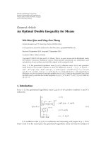
The fi rst set of simulations is designed to verify that the

convergence analysis of (9)isaccurateforL
= 1. For each
simulation run, a ten-by-ten matrix W(0) is generated with
random orthonormal real-valued left and right s ingular vec-
tors and a set of ten singular values uniformly distributed in
the range (0,
√
5). The procedure in (9) is then applied to this
initial matrix. The averaged value of the performance crite-
rion in (31) is computed from 1000 different simulation runs
of the procedure, where m
= n = 10. Shown in Figure 1 is
the evolution of E
{η(t)} in dB, indicating that the algorithm
causes W(t) to converge quickly to an orthonormal matrix if
the singular values of W(0) lie within the algorithm’s mono-
tonic capture region.
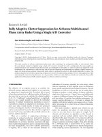
The second set of simulations is designed to verify that
the proposed spatiotemporal procedure in (5)-(6)canbe
used to impose paraunitary constraints on
{W
p
(t)}. In these
simulations, m
= 4, n = 7, L = 11, and {W
p
(0)}is initialized
as
W
p

(0) = Iδ
p−(L−1)/2
+ N
p
, (32)
where N
p
is a sequence of jointly Gaussian matrices having
uncorrelated entries that were zero mean and standard devi-
ation of either sig
= 0.1orsig= 0.01 (see Algorithm 1). One
hundred simulation runs have been averaged to compute the
performance curve shown in Figure 2. Although convergence
of the performance metric is slower than that in the spatial-
only case, the results show that the proposed method does
cause
{W
p
(t)} to converge to a paraunitary system. More-
over, if enough iterations are taken, the performance met-
ric reaches the machine precision of the computing environ-
ment. For small initial perturbations away from paraunitari-
ness, convergence of the algorithm is extremely fast, requir-
ing only a few iterations to decrease the performance metric
by more than 30 dB.
5. APPLICATIONS TO SPATIOTEMPORAL
SUBSPACE ANALYSIS
Consider a sequence of n-dimensional vectors x(k)froma
wide-sense stationary random process in which
R

xx
(l) = E

x(k)x
T
(k − l)

(33)
is the autocorrelation function matrix at lag l.Thegoalof
spatiotemporal subspace analysis is to determine an n-input,
100
90
80
70
60
50
40
30
20
10
0
0 5 10 15 20 25 30
Number of iterations t
Normalized mean-square distance from
orthogonalit y (dB)
Figure 1: Evolution of E{η(t)} for the spatial-only unitary con-
straint algorithm, m
= n = 10, L = 1.
350
300

250
200
150
100
50
0
0 102030405060708090100
Number of iterations t
Signal
= 0.1
Signal
= 0.01
Average performance factor E η(t) (dB)
Figure 2: Evolution of E{η(t)} for the spatiotemporal paraunitary
constraint algorithm, m
= 4, n = 7, and L = 11.
m-output paraunitary system, m<n, with impulse response
W
p
such that the output sequence
y(k)
=
∞

p=−∞
W
p
x(k − p) (34)
has either maximum or minimum total energy E
{y(k)

2
},
where
y(k) denotes the L
2
or Euclidean norm of y(k). If
E
{y(k)
2
} is maximized, then
u(k)
=
∞

q=−∞
W
T
−q
y(k − q) (35)
Scott C. Douglas 7
0
10
4
10
2
10
0
10
2
5000 10000 15000

Number of iterations k
Without adaptive constraint
With adaptive constraint
E ρ
PSA
(k)
(a)
0
100
80
60
40
20
5000 10000 15000
Number of iterations k
Without adaptive constraint
With adaptive constraint
E η(k) (dB)
(b)
Figure 3: Evolutions of (a) E{ρ
PSA
(k)} and (b) E{η(k)} for the spatiotemporal principal subspace algorithms.
is the optimal rank- m linear filtered approximation to the
vector sequence x(k) in a mean-square-error sense. Such
techniques could be used to code multichannel sig nals,
among other applications. Minimization of E
{y(k)
2
} un-
der paraunitary constraints yields the spatiotemporal exten-

sion of the minor subspace analysis task, which is important
for direction of arrival in wideband a rray processing systems
[2, 3, 25, 26].
In [12], simple iterative gradient-based algorithms were
derived for principal and minor subspace analysis tasks. The
spatiotemporal principal subspace algorithm is given by
y(k)
=
L

l=0
W
l
(k)x(k −l), (36)
e(k)
= x(k) −
L

q=0
W
T
L
−q
(k)y(k − q), (37)
W
p
(k +1)=W
p
(k)+μ(k)y(k−L)e
T

(k − p), 0 ≤ p ≤ L,
(38)
where μ(k) is the algorithm step size. This algorithm is
the spatiotemporal extension of the well-known principal
subspace rule [27]. A spatiotemporal minor subspace algo-
rithm is also provided in [12]; it is the spatiotemporal exten-
sion of the self-stabilized algorithm in [14]. The algorithms
are s tochastic-gradient procedures that only approximately
maintain the paraunitary constraints through their adap-
tive behaviors, and their abilit y to maintain the constraint
is linked to the step size chosen for the adaptive procedure.
The proposed iterative procedure in this paper provides
a potential solution to the numerical stabilization of these
gradient-based algor ithms, in which the imposition of the
constraint is met by embedding (5)-(6) within the updates
in (36)–(38). In this algorithm design, we may choose to use
a limited number of iterations of (5)-(6) to improve the nu-
merical performance of the overall algorithm, a choice that
is motivated by the fast convergence of the constraint proce-
dure.Asitisnowshown,even a single iteration of (5)-(6),
when used in conjunction with (36)–(38), enables fast and
accurate convergence to either a principal or minor subspace
estimate, depending on the sign of the step size μ(k). The
simulations that follow explore these issues further.
Consider the example in [12], in which the following
s(k)
= [s
1
(k) s
2

(k)]
T
, s
i
(k), i ∈{1, 2}, are independent zero-
mean Gaussian sequences with autocorrelations r
ss,i
(l) = δ
l
,
x(k)
= x(k)+ν(k),
x(k) =
2

i=1
A
i
x(k −i)+
1

j=0
B
j
s(k − j),
A
1
=
⎡
⎢

⎢
⎢
⎢
⎣
0.38 0.39 −0.22 0.08
0.24
−0.30 −0.03 −0.08
−0.36 −0.20 −0.44 0.02
−0.49 0.16 0.49 −0.17
⎤
⎥
⎥
⎥
⎥
⎦
,
A
2
=
⎡
⎢
⎢
⎢
⎢
⎣
−
0.01 0.01 0.06 0.06
−0.05 0.03 0.04 −0.09
0.02
−0.06 −0.01 0.02

0.05
−0.02 0.01 −0.09
⎤
⎥
⎥
⎥
⎥
⎦
,
B
T
0
=

−
0.02 −0.04 0.07 −0.10
0.05 0.09 0.10 0.06

,
B
T
1
=

−
0.10.0 −0.60.3
−0.40.90.5 −0.2

,
(39)

ν(k)
= [
ν
1
(k) ν
2
(k) ν
3
(k) ν
4
(k)
]
T
,andν
i
(k), i ∈{1, 2, 3, 4}
are independent zero-mean Gaussian signals with r
νν,i
(l) =
σ
2
ν
δ
l
and σ
2
ν
= 10
−4
. We compare the perfor mance of (36)-

(37) with and without one iteration of the adaptive con-
straint procedure in (5)-(6) per time instant, where m
= 2,
n
= 4, L = 14, μ(k) = 0.008 for the algorithm with the adap-
tive constraint method, μ(k)
= 0.005 for the algorithm w i th-
out the adaptive constraint method, and w
ijp
(0) is unity if
i
= j and p = L/2 and is zero otherwise. Note that the step
size for the algorithm with the constraint method is eight
times larger than that used in the simulations in [12], and
the step size for the algorithm without the constraint method
was chosen to obtain the fastest convergence without insta-
bility. S hown in Figures 3(a) and 3(b) are the evolutions of
8 EURASIP Journal on Advances in Signal Processing
0
10
4
10
2
10
0
10
2
5000 10000 15000
Number of iterations k
Without adaptive constraint

With adaptive constraint
E ρ
MSA
(k)
(a)
0
100
80
60
40
20
0
5000 10000 15000
Number of iterations k
Without adaptive constraint
With adaptive constraint
E η(k) (dB)
(b)
Figure 4: Evolutions of (a) E{ρ
MSA
(k)} and (b) E{η(k)} for the spatiotemporal minor subspace algorithms.
the performance factors
ρ
PSA
(k) =


e(k)



2
(40)
and η(k)in(31), respectively, as averaged over one hundred
different simulation runs. As can be seen, the proposed al-
gorithm with a single iteration of the adaptive constraint
method per time instant converges to an accurate subspace
estimate that minimizes the low-rank mean-squared error
criterion. The steady-state value of ρ
PSA
(k) is approximately
3.1
×10
−4
, which is near the minimum value of 2×10
−4
the-
oretically obtainable from the data model. In contrast, the
original spatiotemporal principal subspace algorithm con-
verges more slowly due to the stability limits on the algo-
rithm step size. Larger step sizes caused this latter algorithm
to diverge, that is, it could not maintain the paraunitary con-
straints with a larger step size despite being locally stable to
the constraint space as μ(k)
→ 0. Although not easily proven,
the reason for the poor performance of the original method
for larger step sizes could be due to the delayed-gradient ap-
proximation employed in its derivation, in which past coef-
ficient values appear within the coefficient updates in the er-
ror terms
{e(k−p)}. Such delayed-gradient terms are known

to limit the convergence performance of filtered-gradient al-
gorithms in multichannel active noise control systems [28].
Computing the coefficient update terms using the most re-
cent coefficient values requires more than 3mnL
2
multiply-
accumulates, which for m
 nL
2
is close to the complexity of
a single step of the adaptive constraint procedure. Our novel
adaptive projection method alleviates the convergence dif-
ficulties introduced by the delayed-gradient approximations
and enables the algorithm to properly function for large step
sizes.
We now explore the behavior of (36)-(37) with one it-
eration of the adaptive constraint procedure in (5)-(6)per
time instant when applied to the spatiotemporal minor sub-
space analysis task, in which μ(k) < 0. Note that, without tak-
ing any corrective measures to maintain the coefficient con-
straints, the update in (36)-(37) is unstable in this context
as is the spatial-only principal subspace rule that is obtained
when L
= 1[27]. Figures 4(a) and 4(b) show the evolutions
of the performance factors
ρ
MSA
(k) =



y(k)


2
(41)
and η(k)in(31) for the same input signal model as in the
previous simulation, where μ(k)
=−0.005. The algorithm
without stabilization (dashed lines) quickly diverges. The al-
gorithm with proposed stabilization method performs minor
subspace analysis successfully in this situation, and its con-
vergence speed is much faster than the self-stabilized algo-
rithm described in [12], which requires approximately 30 000
iterations to converge under these same conditions.
6. MULTIDIMENSIONAL EXTENSIONS
Theadaptiveproceduredescribedin(5)-(6)couldbecom-
pactly and approximately defined as
W
p
(t +1)=
3
2
W
p
(t)−
1
2
W
p
(t) ∗W

T
−p
(t) ∗W
p
(t), (42)
where “
∗” denotes discrete-time convolution over the in-
dex p and the all-important truncation issues associated with
the finite-length convolutions have been ignored. This form
of the adaptive procedure inspires us to consider versions
of the algorithm for h igher-dimensional data, such as im-
ages, video, and hyperspectral imagery. It is reasonable to as-
sume that, with an appropriately defined convolution opera-
tor, one could extend the procedure in (5)-(6) to these other
data types. For example, consider an n-input, m-output two-
dimensional (2D) FIR linear filter of the form
y(k, l)
=
L−1

p=0
L
−1

q=0
W
p,q
x(k − p, l − q), (43)
where
{W

p,q
} contain the coefficients of the multichannel
system. A multichannel 2D paraunitary filter would impose
the constraints
min{L−1,L−1+k}

p=max{0,k}
min{L−1,L−1+l}

q=max{0,l}
W
p,q
W
T
p
−k,q−l
= I
m
δ
k
δ
l
, −M ≤{k, l}≤M
(44)
Scott C. Douglas 9
on the coefficients of the linear system. Translating the pro-
posed multichannel one-dimensional paraunitary constraint
procedure to this two-dimensional structure, we obtain the
update in polynomial form as
W

t+1

z
1
, z
2

=
3
2
W
t

z
1
, z
2

−
1
2


W
t

z
1
, z
2


W
T
t

z
−1
1
, z
−1
2

(L−1)/2
−(L−1)/2
W
t

z
1
, z
2


L−1
0
,
(45)
where
W
t


z
1
, z
2

=
L−1

p=0
L
−1

q=0
W
p,q
(t)z
−p
1
z
−q
2
(46)
is the 2D z-transform of
{W
p,q
(t)} and [·]
N
M
here denotes

truncation of its two-dimensional polynomial argument to
the individual powers for z
1
and z
2
within the range [M, N].
We can illustrate the usefulness of this particular procedure
with a simple video coding example, described using the
MATLAB technical computing environment.
Consider the task of designing a three-input (n
= 3),
one-output (m
= 1) paraunitary system for a set of three
similar images, in which the convolution kernel for each im-
age is of size (L
×L), where L is odd. Let W1, W2, and W3de-
note the corresponding 2D convolution kernel matrices, such
that L
= 3, and W
t
(z
1
, z
2
)isa(1× 3) vector of polynomials
in z
1
and z
2
. Then, the following MATLAB code employing

the function filter2 can be used to impose paraunitary con-
straints on the filter coefficient set
{W1, W2, W3}:
for t = 1:numiter
C
= filter2(W1,W1) + filter2(W2,W2)
+ filter2(W3,W3)
W1
= 3/2∗W1 - 1/2∗filter2(C,W1);
W2
= 3/2∗W2 - 1/2∗filter2(C,W2);
W3
= 3/2∗W3 - 1/2∗filter2(C,W3);
end
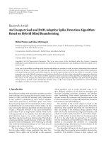
To illustrate that this procedure works as designed, con-
sider a simple video compression example. Given an image
sequence, we first calculate a sequence of difference images.
For every three difference images, we estimate a principal
component image y(k, l) by maximizing the output power
of the image pixels from the three-input, one-output parau-
nitary system while imposing a par aunitary constraint via
the above adaptive procedure. In this procedure, we used
a “center-spike” initialization strategy, where W1andW3
weresettozeromatricesandW2 had one non-zero value
in the center of its impulse response. We then reconstruct
the first and third difference images from the single princi-
pal component image y(k, l) using W1andW3, resulting in
(a)
(b)
Figure 5: Reconstruction of the Cronkite sequence using 2D adap-

tive paraunitary filters (left-original, right-reconstructed).
the reconstructed difference images u
1
(k, l)andu
3
(k, l), re-
spectively. Finally, we use the reconstructed difference images
to calculate two intermediate frames from every third “key”
frame within the image sequence using adds and subtracts,
respectively. The result is a compressed image sequence, be-
cause for every three frames, one only needs on average one
“key” image frame, one principal component image frame
y(k, l), and the two filtering kernels W1andW3torep-
resent three images within the sequence. Of course, such a
compression scheme cannot compete with more-common
motion-based image compression schemes, but the success
of a 2D adaptive paraunitary filter in such an application il-
lustrates the capability and flexibility of the proposed con-
straint method.
We applied the above video compression scheme to a spa-
tially downsampled version of the Cronkite video sequence
obtained from the USC SIPI database, where L
= 3. In this
case, the images were downsampled to size 128
× 128 pix-
els, and a gradient-based principal component analysis pro-
cedure was used in conjunction with the adaptive 2D parau-
nitary constraint procedure with numiter
= 50 to maximize
the output powers in the principal component images. From

the sixteen-frame sequence, the ten resulting reconstructed
images had an average PSNR of 26.75 dB with a standard de-
viation of 2.17 dB. Shown in Figure 5 are the original (left)
and reconstructed (right) frames from this procedure from
the eleventh (top) and twelfth (bottom) frames, respectively.
As can be seen, the quality of reconstruction is high, and the
proposed paraunitary constraint method can be employed to
solve this approximation task.
10 EURASIP Journal on Advances in Signal Processing
The above paraunitar y constraint procedure can be ex-
tended to the general N-dimensional filtering task. Define
the sets Z
N
={z
1
, z
2
, , z
N
} and Z
−1
N
={z
−1
1
, z
−1
2
, , z
−1

N
}.
Then, the polynomial representation of the general algo-
rithm is
W
t+1

Z
N

=
3
2
W
t
(Z
N
)
−
1
2


W
t

Z
N

W

T
t

Z
−1
N

(L−1)/2
−(L−1)/2
W
t

Z
N


L−1
0
,
(47)
where
W
t

Z
N

=
N


i=1
L
−1

p
i
=0
W
p
1
,p
2
, ,p
N
(t)
N

j=1
z
−p
j
j
(48)
is the N-dimensional z-transform of W
p
1
,p
2
, ,p
N

(t)and[·]
P
M
denotes truncation of its N-dimensional polynomial argu-
ment to the individual powers for z
1
through z
N
within the
range [M, P]. One possible application for this method is the
representation of multiple video sequences via subspace pro-
cessing, a subject of cur rent study.
7. CONCLUSIONS
In this paper, we have described an adaptive scheme for im-
posing paraunitary constraints on a multichannel linear sys-
tem. The procedure is straightforward to implement, and its
convergence is locally quadratic to the constraint space. We
have demonstrated that the technique can be used to ob-
tain improved convergence p erformance from existing sim-
ple gradient-based spatiotemporal subspace analysis meth-
ods, and we have shown how to extend the concept to higher-
dimensional data sets through a simple video compression
task. Extensions of these ideas are being applied to the con-
volutive blind source separation task; see [29] for additional
details on these procedures.
REFERENCES
[1] B. Farhang-Boroujeny and S. Nooshfar, “Adaptive phase
equalization using all-pass filters,” in Proceedings of IEEE In-
ternat ional Conference on Communications (ICC ’91), vol. 3,
pp. 1403–1407, Denver, Colo, USA, June 1991.

[2] P. Loubaton and P. A. Regalia, “Blind deconvolution of multi-
variate signals by using adaptive FIR lossless filters,” in Pro-
ceedings of the European Signal Processing Conference (EU-
SIPCO ’92), pp. 1061–1064, Brussels, Belgium, August 1992.
[3] P. A. Regalia and P. Loubaton, “Rational subspace estimation
using adaptive lossless filters,” IEEE Transactions on Signal Pro-
cessing, vol. 40, no. 10, pp. 2392–2405, 1992.
[4] T. J. Lim and M. D. Macleod, “Adaptive allpass filtering for
nonminimum-phase system identification,” IEE Proceedings–
Vision, Image, and Signal Processing, vol. 141, no. 6, pp. 373–
379, 1994.
[5] M. K. Tsatsanis and G. B. Giannakis, “Principal component fil-
ter banks for optimal multiresolution analysis,” IEEE Transac-
tions on Signal Processing, vol. 43, no. 8, pp. 1766–1777, 1995.
[6] P. A. McEwen and J. G. Kenney, “Allpass forward equalizer for
decision feedback equalization,” IEEE Transactions on Magnet-
ics, vol. 31, no. 6, part 1, pp. 3045–3047, 1995.
[7] E. Abreu, S. K. Mitra, and R. Marchesani, “Nonminimum
phase channel equalization using noncausal filters,” IEEE
Transactions on Signal Processing, vol. 45, no. 1, pp. 1–13, 1997.
[8] A. Kirac and P. P. Vaidyanathan, “Theory and design of opti-
mum FIR compaction filters,” IEEE Transactions on Signal Pro-
cessing, vol. 46, no. 4, pp. 903–919, 1998.
[9] P. Moulin and M. K. Mihcak, “Theory and design of signal-
adapted FIR paraunitary filter banks,” IEEE Transactions on
Signal Processing, vol. 46, no. 4, pp. 920–929, 1998.
[10] B. Xuan and R. I. Bamberger, “FIR principal component filter
banks,” IEEE Transactions on Signal Processing, vol. 46, no. 4,
pp. 930–940, 1998.
[11] X. Sun and S. C. Douglas, “Self-stabilized adaptive allpass fil-

ters for phase equalization and approximation,” in Proceed-
ings of IEEE International Conference on Acoustics, Speech, and
Signal Processing (ICASSP ’00), vol. 1, pp. 444–447, Istanbul,
Turkey, June 2000.
[12] S. C. Douglas, S I. Amari, and S Y. Kung, “Gradient adaptive
paraunitary filter banks for spatio-temporal subspace analysis
and multichannel blind deconvolution,” Journal of VLSI Signal
Processing, vol. 37, no. 2-3, pp. 247–261, 2004.
[13] T P. Chen, S I. Amari, and Q. Lin, “A unified algorithm
for principal and minor components extraction,” Neural Net-
works, vol. 11, no. 3, pp. 385–390, 1998.
[14] S. C. Douglas, S Y. Kung, and S I. Amari, “A self-stabilized
minor subspace rule,” IEEE Signal Processing Letters, vol. 5,
no. 12, pp. 328–330, 1998.
[15] M. A. Hasan, “Natural gradient for minor component extrac-
tion,” in Proceedings of IEEE International Symposium on Cir-
cuits and Systems (ISCAS ’05), vol. 5, pp. 5138–5141, Kobe,
Japan, May 2005.
[16] J. H. Manton, U. Helmke, and I. M. Y. Mareels, “A dual pur-
pose principal and minor component flow,” Systems and Con-
trol Letters, vol. 54, no. 8, pp. 759–769, 2005.
[17] K. Fan and A. J. Hoffman, “Some metric inequalities in the
space of matrices,” Proceedings of the American Mathematical
Society, vol. 6, no. 1, pp. 111–116, 1955.
[18] Y. Hua, “Asymptotical orthonormalization of subspace ma-
trices without square root,” IEEE Signal Processing Magazine,
vol. 21, no. 4, pp. 56–61, 2004.
[19] S. C. Douglas, S I. Amari, and S Y. Kung, “On gradient adap-
tation with unit-norm constraints,” IEEE Transactions on Sig-
nal Processing

, vol. 48, no. 6, pp. 1843–1847, 2000.
[20] J. H. Manton, “Optimization algorithms exploiting unitary
constraints,” IEEE Transactions on Signal Processing, vol. 50,
no. 3, pp. 635–650, 2002.
[21] A. Bjorck and C. Bowie, “An iterative algorithm for computing
the best estimate of an orthogonal matrix,” SIAM Journal on
Numerical Analysis, vol. 8, no. 2, pp. 358–364, 1971.
[22] A. Hyvarinen, J. Karhunen, and E. Oja, Independent Compo-
nent Analysis, John Wiley & Sons, New York, NY, USA, 2001.
[23] S. C. Douglas and A. Cichocki, “Neural networks for blind
decorrelation of signals,” IEEE Transactions on Signal Process-
ing, vol. 45, no. 11, pp. 2829–2842, 1997.
[24] T. Chen and Q. Lin, “Dynamic behavior of the whitening pro-
cess,” IEEE Signal Processing Letters, vol. 5, no. 1, pp. 25–26,
1998.
[25] B. Porat and B. Friedlander, “Estimation of spatial and spec-
tral parameters of multiple sources,” IEEE Transactions on In-
formation Theory, vol. 29, no. 3, pp. 412–425, 1983.
Scott C. Douglas 11
[26] B. Ottersten and T. Kailath, “Direction-of-arrival estimation
for wide-band signals using the ESPRIT algorithm,” IEEE
Transactions on Acoustics, Speech, and Signal Processing, vol. 38,
no. 2, pp. 317–327, 1990.
[27] E. Oja and J. Karhunen, “On stochastic approximation of the
eigenvectors and eigenvalues of the expectation of a random
matrix,” Journal of Mathematical Analysis and Applications,
vol. 106, no. 1, pp. 69–84, 1985.
[28] S. C. Douglas, “Fast implementations of the filtered-X LMS
and LMS algorithms for multichannel active noise control,”
IEEE Transactions on Speech and Audio Processing, vol. 7, no. 4,

pp. 454–465, 1999.
[29] S. C. Douglas, H. Sawada, and S. Makino, “A spatio-temporal
fastica algorithm for separ ating convolutive mixtures,” in Pro-
ceedings of IEEE International Conference on Acoustics, Speech
and Signal Processing (ICASSP ’05), vol. 5, pp. 165–168,
Philadelphia, Pa, USA, March 2005.
Scott C. Douglas is an Associate Professor
in the Department of Electrical Engineering
at Southern Methodist University, Dallas,
Tex, and is the Associate Director for the In-
stitute for Engineering Education at SMU.
He received his B.S., M.S., and Ph.D. de-
grees from Stanford University. Dr. Douglas
is a recognized expert in the fields of adap-
tive filters, blind source separation, and ac-
tive noise control, having authored or coau-
thored two books, six book chapters, and over 150 papers in jour-
nals and conference proceedings. He is a recipient of an NSF Career
(Young Investigator) Award and has received significant research
funding from the US Army, DARPA, other US governmental orga-
nizations, the State of Texas, and numerous companies. He is highly
active in professional societies and has served as an Associate Editor
for both the IEEE Transactions on Signal Processing and the IEEE
Signal Processing Letters. He has served on the organizing com-
mittees of numerous international conferences and workshops as
Technical Chair, Publications Chair, and Exhibits Chair, and is the
General Chair of the 2010 International Conference on Acoustics,
Speech, and Signal Processing. He has given many keynote and in-
vited lectures as well as short courses on topics ranging from adap-
tive signal processing and control to innovative engineering edu-

cation methods. Most recently, he has coauthored textbooks and
developed materials and technology for the Infinity Project, a mul-
tifaceted effort to establish a United States engineering curriculum
at precollege educational le vels. Dr. Douglas is a frequent consul-
tant to industry, a Senior Member of the IEEE, and a Member of
both Phi Beta Kappa and Tau Beta Pi.