Báo cáo hóa học: " Research Article Accurate Tempo Estimation Based on Harmonic + Noise Decomposition" pot

Hindawi Publishing Corporation
EURASIP Journal on Advances in Signal Processing
Volume 2007, Article ID 82795, 14 pages
doi:10.1155/2007/82795
Research Article
Accurate Tempo Estimation Based on
Harmonic + Noise D ecomposition
Miguel Alonso, Ga
¨
el Richard, and Bertrand David
T
´
el
´
ecom Paris,
´
Ecole Nationale Sup
´
erieure des T
´
el
´
ecommunications, Groupe des
´
Ecoles des T
´
el
´
ecommunications (GET),
46 Rue Barrault, 75634 Paris Cedex 13, France
Received 2 December 2005; Revised 19 May 2006; Accepted 22 June 2006

Recommended by George Tzanetakis
We present an innovative tempo estimation system that processes acoustic audio signals and does not use any high-level musical
knowledge. Our proposal relies on a harmonic + noise decomposition of the audio signal by means of a subspace analysis method.
Then, a technique to measure the degree of musical accentuation as a function of time is developed and separately applied to
the harmonic and noise parts of the input signal. This is followed by a periodicity estimation block that calculates the salience of
musical accents for a large number of potential periods. Next, a multipath dynamic programming searches among all the potential
periodicities for the most consistent prospects through time, and finally the most energetic candidate is selected as tempo. Our
proposal is validated using a manually annotated test-base containing 961 music signals from various musical genres. In addition,
the performance of the algorithm under different configurations is compared. The robustness of the algorithm when processing
signals of degraded quality is also measured.
Copyright © 2007 Miguel Alonso et al. This is an open access article distributed under the Creative Commons Attribution License,
which permits unrestricted use, distribution, and reproduction in any medium, provided the original work is properly cited.
1. INTRODUCTION
The continuously growing size of digital audio information
increases the difficulty of its access and management, thus
hampering its practical usefulness. As a consequence, the
need for content-based audio data parsing, indexing, and re-
trie val techniques to make the digital information more read-
ily available to the user is becoming critical. It is then not
surprising to observe that automatic music analysis is an in-
creasingly active research area. One of the subjects that has
attracted much attention in this field concerns the extraction
of rhythmic information from music. In fact, along with har-
mony and melody, rhythm is an intrinsic part of the music. It
is difficult to provide a rigorous universal definition, but for
our needs we can quote Parncutt [1]: “a musical rhythm is an
acoustic sequence evoking a sensation of pulse” which refers
to all possible rhythmic levels, that is, pulse rates, evoked in
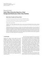
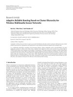
the mind of a listener (see Figure 1). Of particular impor-
tance is the beat, also called tactus or foot-tapping rate, which

can be interpreted as a comfortable middle point in the met-
rical hierarchy closely related to the human’s natural move-
ment [2]. The concept of phenomenal accent hasagreatrel-
evance in this context, Lerdahl and Jackendoff [3] define it
as “the moments of musical stress in the raw signal (who)
serve as cues from which the listener attempts to extrapolate
a regular pattern.” In practice, we consider as phenomenal ac-
cents all the discrete events in the audio stream where there
is a marked change in any of the perceived psychoacoustical
properties of sound, that is, loudness, timbre, and pitch.
Metrical analysis is receiving a strong interest from the
community because it plays an important role in many ap-
plications: automatic rhythmic alignment of multiple instru-
ments, channels, or musical pieces; cut and paste operations
in audio editing [ 4]; automatic musical accompaniment [5],
beat-driven special effects [6, 7], music transcription [8], or
automatic genre classification [9].
A number of studies on metrical analysis were devoted
to symbolic input usually in MIDI or other score format
[10, 11]. However, since the vast majority of musical sig-
nals are available in raw or compressed audio format, a large
number of recent work focus on methods that directly pro-
cess the time waveform of the audio signal. As pointed out
by Klapuri et al. [8], there are three basic problems that need
to be addressed in a successful metrical analysis system. First,
the degree of musical stress as a function of time has to be
measured. Next, the periods and phases of the underlying
2 EURASIP Journal on Advances in Signal Processing
3
4

Higher
Lower
Rhythmic
levels
Figure 1: Example showing how the rhythmic structure of music can be decomposed in rhythmic levels formed by equidistant pulses. There
is a double relationship between the lowest rhythmic level and the next higher rhythmic level, on the contrary there is a triple relationship
between the highest rhythmic level and the next lower level.
metrical pulses have to be estimated. Finally, the system has
to choose the pulse level which corresponds to the tactus or
some other specifically designated metrical level.
A large variety of approaches have already been investi-
gated. Histogram models are based on the computation of the
interonset intervals (IOIs) histograms from which the beat
period is estimated. The IOIs are obtained by detecting the
precise location of onsets or phenomenal accents and the de-
tectors often operate on subband signals (see, e.g., [12–14]
or [15]). The so-called detection function model does not aim
at precisely extracting onset positions, but rather at obtain-
ing a smooth profile, usually known as the “detection func-
tion,” which indicates the possibility of finding an onset as a
function of time. This profile is usually built from the time
waveform envelope [16]. Periodicity analysis can be carried
out by a bank of oscillators based on comb filters [8, 17]orby
other periodicit y detectors [18, 19]. Probabilistic models sup-
pose that onsets are random and exploit Bayesian approaches
such as particle filtering to find beat locations [20, 21]. Cor-
relative approaches have also been proposed, see [22]fora
method that compares the detection function with a pulse-
train signal and [23] for an autocorrelation-based algorithm.
The goal of the present work is to describe a method

which performs metrical analysis of acoustic music record-
ings at one pulsation le vel: the tactus. The proposed model
is an extension of a previous system that was ranked first in
the tempo contest of the 2nd Annual Music Information Re-
trieval Evaluation eXchange (MIREX) [24]. Our model in-
cludes several innovative aspects including:
(i) the use of a signal/noise subspaces decomposition,
(ii) the independent processing of its deterministic (sum
of sinusoids) and noise components for estimating
phenomenal accents and their respective periodicity,
(iii) the development of an efficient audio onset detector,
(iv) the exploitation of a multipath dynamic programming
approach to highlight consistent estimates of the tac-
tus and which allows the estimation of multiple con-
current tempi.
The paper is organized as follows. Section 2 describes the
different elements of our algorithm, then Section 3 presents
the experimental results and compares the proposed model
with two reference methods. Finally, Section 4 summarizes
Audio
signal
Filter bank
Subspace
projection
Subspace
projection
Musical
stress
estimation
Musical

stress
estimation
Periodicity
estimation
Periodicity
estimation
Dynamic programming
Metrical paths analysis
Tactus
estimation
2
2
2
2

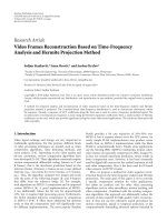
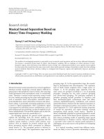
Figure 2: Overview of the tempo estimation system.
the achievements of our system and discusses possible direc-
tions for future improvements.
2. DESCRIPTION OF THE ALGORITHM
The architecture of our tempo estimation system is provided
in Figure 2. First, the audio signal is split in P subbands sig-
nals which are further decomposed into deterministic (sum
of sinusoids) and noise components. From these signals, de-
tection functions which measure in a continuous manner the
degree of musical accentuation as a function of time are ex-
tracted and their periodicity is then estimated by means of
several different algorithms. Next, a multipath dynamic pro-
gramming algorithm permits to robustly track through time
several pulse periods from which the most persistent is cho-
sen as the tactus. The different building blocks of our system

are detailed below. Note that throughout the rest of the pa-
per, it is assumed that the tempo of the audio signal is stable
Miguel Alonso et al. 3
over the duration of the observation window. In addition,
we suppose that the tactus lies between 50 and 240 beats per
minute (BPM).
2.1. Harmonic + noise decomposition based
on subspace analysis
In this part, we describe a subspace analysis technique (some-
times referred to as high-resolution methods) which models
a signal as a sum of sinusoidal components and noise.
Our main motivation to decompose the music signal is
the idea of emphasizing phenomenal accents by separating
them f rom the surrounding disturbing events, we explain
this idea using an example. When processing a piano signal
(percussive or plucked string sounds in general), the sinu-
soidal components hamper the detection of the nonstation-
ary mechanical noise of the attack, in this case the sound of
the hammer hitting the cords. Conversely, when processing
a violin signal (bowed strings or wind instrument sounds in
general), the nonstationary friction noise of the bow rubbing
the cords hampers the detection of the sinusoidal compo-
nents.
The decomposition procedure used in the present work
refers to the first two blocks of the scheme presented in
Figure 2 and is founded on the research carried out by
Badeau et al. [25, 26 ]. Related work using such methods in
the context of metrical analysis for music signals has been
previously proposed in [19]. Let x(n), n
∈ Z, be the real an-

alyzed signal, modeled as the sum
x( n)
= s(n)+w(n), (1)
where
s(n)
=
2M

i=1
α
i
z
n
i
(2)
is referred to as the deterministic part of x.Theα
i
= 0are
the complex amplitudes bearing magnitude and phase infor-
mation and the z
i
are the complex poles z
i
= e
d
i
+ j2πf
i
,where
f

i
∈ [−1/2, 1/2[ are the frequencies with f
i
= f
k
for all i = k
and d
i
∈ R are the damping factors. It can be noted that
since s is a real sequence, z
i
’s and α
i
’s can be grouped in M
pairs of conjugate values. Subspace analysis techniques rely
on the following property of the L-dimensional data vector
s(n)
= [s(n − L +1), , s(n)]
T
(with usually 2M  L):
it belongs to the 2M-dimensional subspace spanned by the
basis
{v(z
k
)}
k=0, ,2M−1
,wherev(z) = [
1 z
··· z
L−1

]
T
is
the Vandermonde vector a ssociated with a nonzero complex
number z. This subspace is the so-called signal subspace.As
a consequence, v(z
k
) ⊥ span (W
⊥
), where W denotes an
L
× 2M matrix spanning the signal subspace and W
⊥
an
N
× (N − 2M) matrix spanning its orthogonal complement,
referred to as the noise subspace. The harmonic + noise de-
composition is performed by projecting the signal x,respec-
tively, on the signal subspace and the noise subspace.
Let the symmetric L
×L real Hankel matrix H
s
be the data
matrix:
H
s
=
⎡
⎢
⎢

⎢
⎢
⎣
s(0) s(1) ··· s(L − 1)
s(1) s(2)
··· s(L)
.
.
.
.
.
.
.
.
.
.
.
.
s(L
− 1) s(L) ··· s(N − 1)
⎤
⎥
⎥
⎥
⎥
⎦
,(3)
where N
= 2L − 1, with 2M ≤ L.SinceeachcolumnofH
s

belongs to the same 2M-dimensional subspace, the matrix is
of rank 2M, and thus is rank-deficient. Its eigenvalue decom-
position (EVD) yields
H
s
= UΛ
s
U
H
,(4)
where U is an orthonormal matrix, Λ
s
is the L × L diago-
nal matrix of the eigenvalues, L
− 2M of which are zeros. U
H
denotes the Hermitian transpose of U. T he 2M-dimensional
space spanned by the columns of U corresponding to the
nonzero entries of Λ
s
is the signal subspace.
Because of the surrounding additive white noise, H
x
is
full rank and the signal subspace U
S
is formed by the 2M-
dominant eigenvectors of H
x
, that is, the column of U asso-

ciated to the 2M eigenvalues having the highest magnitudes.
In practice, we observe that the noisy sequence x(n)and
its harmonic par t can be obtained by projecting x(n)ontoits
signal subspace as follows:
s
= U
S
U
H
S
x. (5)
A remarkable property of this method is that for calculat-
ing the noise part of the signal, the estimation and subtrac-
tion of the sinusoids is not required explicitly. The noise is
obtained by projecting x(n) onto the noise subspace:
w
= x − s =

I − U
S
U
H
S

x. (6)
Subspace tracking
Since the harmonic + noise decomposition of x(n)involves
the calculation of one EVD of the data matrix H
x
at every

time step, decomposing the whole signal would require a
highly demanding computational burden. In order to reduce
this cost, there exist adaptive methods that avoid the com-
putation of the EVD [27], a survey of such methods can be
found in [26]. For the present work, we use an iterative algo-
rithm called sequential iteration [25], show n in Algorithm 1.
Assuming that it converges faster than the var iations of the
signal subspace, the algorithm operation involves two auxil-
iary matrices at every time step A(n)andR(n), in addition
of a skinny QR factorization. The harmonic and noise parts
of the whole signal x(n) can be computed by means of an
overlap-add method.
(1) The analysis window is recursively time-shifted. In
practice,wechooseanoverlapof3L/4.
(2) The signal subspace U
S
is tracked by means of the pre-
viously mentioned sequential iteration algorithm pre-
sented in Algorithm 1.
4 EURASIP Journal on Advances in Signal Processing
Initialization: U
S
=

I
2M
0
(N−2M)×2M

For each time step n iterate:

(1) A(n)
= H(n)U
S
(n − 1) fast matrix product
(2) A(n)
= U
S
(n)R(n) skinny QR factorization
Algorithm 1: Sequential iteration EVD algorithm.
(3) The harmonic s and noise w vectors are computed ac-
cording to (5)and(6).
(4) Finally, consecutive harmonic and noise vectors are
multiplied by a Hann window and, respectively, added
to the harmonic and noise parts of the signal.
The overall computational complexity of the harmonic +
noise decomposition for each analysis block is that of step
(2), which is the most computationally demanding task
of the whole metrical analysis system. Its complexity is
O(Ln(n +log(L))).
Subspace analysis methods rely on two principles. From
one part, they assume that the noise is white and secondly,
that the order of the model (number of sinusoids) is known
in advance. Both of these premises are not usually satisfied in
most applications.
A practical remedy to overcome the colored noise prob-
lem consists of using a preaccentuation filter
1
and in sepa-
rating the signal in frequency bands, which has the effect of
leading to a (locally) whiter noise in each channel. The input

signal x(n) is decomposed into P
= 8 uniform subband sig-
nals x
p
(n), where p = 0, , P−1. Subband decomposition is
carried out using a maximally decimated cosine-modulated
filter bank [28], where the prototype filter is implemented as
a 150th-order FIR filter with 80 dB of rejection in the stop
band. Using such a highly selective filter is relevant because
subspace projection techniques are very sensitive to spurious
sinusoids.
Estimating the exact number of sinusoids present in a
given signal is a considerably difficult task and a large ef-
fort has been devoted to this problem, for instance [29, 30].
For our application, we decided to slightly overestimate the
model order since according to Badeau [26, page 54] it has a
small impact in the algorithm performance compared to an
underestimation. Another important advantage of the band-
wise processing approach is that there are less sinusoids per
subband (compared to the full-band signal) which allows at
the same time to reduce the overall computational complex-
ity, that is, we deal with more matrices but P-times smaller
in size.
In this way, further processing in the subbands is the
same for all frequency channels. The output of the decom-
1
Since the power spectral density of audio signals is a decreasing function
of frequency, the use of a preaccentuation filter that tends to flatten this
global trend is necessary. In our implementation we use the same filter as
in [26], that is, G(z)

= 1 − 0.98z
−1
.
position stage consists of two signals: s
p
(n) carrying the har-
monic and w
p
(n) the noise part of x
p
(n).
2.2. Calculation of a musical stress profile
The harmonic + noise decomposition previously descr ibed
can be seen as a front end that performs “signal condition-
ing,” in this case it consists of decomposing the input signal
in several harmonic and noise components prior to rhythmic
processing.
In the metrical analysis community, there exists an im-
plicit consensus about decomposing the music signal in sub-
bands prior to conducting rhythm analysis. According to
experiments carried out by Scheirer [17], there exists no opti-
mal decomposition since many subband layouts lead to com-
parable satisfactory results. In addition, he argues that a “psy-
choacoustic simplification” consisting of a simple envelope
extraction in a number of subbands is sufficient to extract
pulse and meter information from music signals. The tempo
estimation system herein proposed is built upon this princi-
ple.
The concept of phenomenal accent as a discrete sound
event plays a fundamental role in metrical analysis. Humans

hear them in a hierarchical structure, that is, a phenomenal
accent is related to a motif, several motifs are clustered into a
pattern and a musical piece is formed of several patterns that
may be different or not. In the present work, we attempt to be
acute (in a computational sense) to the physical events in an
audio signal related to the moments of musical stress, such
as magnitude changes, harmonic changes, and pitch leaps,
that is, acoustic effects that can be heard and are musically
relevant for the listener. The attribute of being sensitive to
these events does not necessarily imply the need of a specific
algorithm for detecting harmonic or pitch changes, but solely
a method which reacts to variations in these charac teristics.
In practice, calculating a profile of the musical stress
present in a music signal as a function of time is intimately
related to the task of detecting onsets. Robust onset detection
for a wide range of music signals has proven to be a difficult
task. In [31], Bello et al. provide a survey of the most com-
monly used methods. While we propose an approach that
exploits previous research [16, 22] as a starting point, it sig-
nificantly improves the calculation of the spectral energy flux
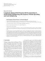
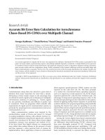
(SEF) or spect ral difference [32]. See Figure 3 for an overview
of the proposed method. As in the previous section, the algo-
rithm will be presented for a single subband case and only for
the harmonic component s
p
(n), since the same procedure is
followed for the noise part w
p
(n) and the rest of the sub-
bands.

Spectral energy flux
The method that we present resides on the general assump-
tion that the appearance of an onset in an audio stream leads
to a variation in the signal’s frequency content. For example,
in the case of a violin producing pitched notes, the resulting
signal will have a strong fundamental frequency that leaps
in time as wel l as the related harmonic components at in-
teger multiples of the fundamental attenuating as frequency
Miguel Alonso et al. 5
Channel
processing
Channel
processing
Detection
function
Lowpass
filtering
Nonlinear
compression
Derivative
calculation
HWR
Channel processing
STFT
.
.
.
.
.
.

s
p
(n)
or
w
p
(n)

Figure 3: Overview of the system to estimate musical stress.
increases. In the case of a percussive instrument, the resulting
signal will tend to have sharp energy boosts. The harmonic
component s
p
(n) is analyzed using the STFT, leading to

S
p
(m, k) =
∞

n=−∞
w(Mm − n)s
p
(n)e
− j(2π/N)kn
,(7)
where w(n) is a finite-length sliding window, M the hop size,
m the time (frame) index, and k
= 0, , N − 1 the frequency
channel (bin) index. To detect the above-mentioned varia-

tions in the frequency content of the audio signal, previous
methods have proposed the calculation of the derivative of

S
p
(m, k)withrespecttotime,
E
p
(l, k) =

m
h(l − m)G
p
(m, k), (8)
where E
p
(l, k) is known as the spectral energy flux (SEF),
h(m) is an approximation to an ideal differentiator
H

e
j2πf


j2πf,(9)
G
p
(m, k) = F





S
p
(m, k)



(10)
is a transformation that accentuates some of the psychoa-
coustically relevant properties of

S
p
(m, k).
In solving many physical problems by means of numeri-
cal methods, it is a challenge to seek derivatives of functions
given in discrete points. For example, in [16, 22] authors pro-
pose a first-order difference with h
= [1, −1], which is a
rough approximation to an ideal differentiator. In this paper,
we use a differentiator filter h(m)oforder2L based on the
formulas for central differentiation developed by Dvornikov
in [33] which provides a much closer approximation to (9).
Other efficient differentiator filters can be used providing
comparable results, for instance, FIR filters obtained by the
Remez method [34]. The underly ing principle of the pro-
posed digital differentiator is the calculation of an interpo-
lating polynomial of order 2L passing through 2L+1 discrete
points, which is used to find the derivative approximation. A

comprehensive description of the method and its accuracy to
approximate (9)canbefoundin[33]. The analytical expres-
sion to compute the first L coefficients of an antisymmetric
FIR differentiator is given by g(i)
= 1/iα(i)with
α(i)
=
L

j=1
j
=i

1 −
i
2
j
2

(11)
and i
= 1, , L. The coefficients of h(m)aregivenby
h
=

−
g(L), ,0, , g(L)

. (12)
In our proposal, the transfor mation G(m, k)calculatesaper-

ceptually plausible power envelope for frequency channel k
and is formed of t wo steps. First, psychoacoustic research on
computational models of mechanical to neural transduction
[35] shows that the auditory nerve adaptation response fol-
lowing a sudden stimulus change can be characterized as the
sum of two exponential decay functions:
φ(m)
= αe
−m/T
1
+ βe
−m/T
2
,form ≥ 0, (13)
formed by a rapid-decline component with time constant
(T
1
) in the order of 10 milliseconds and a slower short-term
decline with a time constant (T
2
) in the region of 70 millisec-
onds. This adaptation function performs energy integration,
emphasizing the most recent stimulus but masking rapid
modulations. From a signal processing standpoint, this can
be viewed as two smoothing low-pass filters whose impulse
response has a discontinuity that preserves edge sharpness
and avoids dulling signal attacks. In practice, the smoothing
window is implemented as a second-order IIR filter with z-
transform,
Φ(z)

=
α + β −

αz
2
+ βz
1
z
−1

1 −

z
1
+ z
2

z
−1
+ z
1
z
2
z
−2
, (14)
where T
1
= 15 milliseconds, T
2

= 75 milliseconds, α = 1,
β
= 5, z
1
= e
−1/T
1
,andz
2
= e
−1/T
2
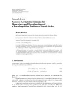
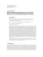
. Figure 4 shows the role
of the energy integration function after convolving it with a
pitched channel of a signal’s spectrogram representation.
The second part of the envelope extraction consists of a
logarithmic compression. This operation has also a percep-
tual relevance since the logarithmic difference function gives
the amount of change in a signal’s intensity in relation to its
level, that is,
d
dt
log I(t)
=
ΔI(t)
I(t)
. (15)
This means that the same amount of increase is more promi-
nent in a quiet signal [16, 36 ].
In practice, the algorithm implementation is straight-

forward, and is carried out as presented in Figure 3.The
STFT in (7) is computed using an N-point fast Fourier trans-
form (FFT). The absolute value of every frequency chan-
nel
|

S(m, k)| is convolved with φ(m). The smoothing opera-
tion is followed by a logarithmic compression. The resulting
6 EURASIP Journal on Advances in Signal Processing
0
0.5
1
00.511.522.5
Amplitude
Time (s)
(a)
0
0.5
1
00.511.522.5
Amplitude
Time (s)
(b)
Figure 4: The smoothing effect of the energy integration function
emphasizes signal attacks but masks rapid modulations. The image
shows a pitched frequency channel corresponding to piano signal
(a) before smoothing and (b) after smoothing.
G(m, k)isgivenby
G(m, k)
= log

10


i



S(i, k)


φ(m − i)

. (16)
At those time instants where the frequency content of
s
p
(n) changes and new frequency components appear, E(l, k)
exhibits positive peaks whose amplitude is proportional to
the energy and rate of change of the new components. In
a similar way, when frequency components disappear from
s
p
(n), the SEF exhibits negative peaks, mar king the offset of a
musical event. Since we are only interested in onsets, we ap-
ply a half-wave rectification (HWR) to E(l, k), that is, only
positive values are taken into account. To find a global sta-
tionarity profile v(l), better know n as the detection function,
contributions from all channels are integrated across fre-
quency,
v(l)

=

k
E(l,k)>0
E(l, k). (17)
v(l) displays sharp p e aks at transients and note onsets, those
instants where the positive energy flux is large. Figure 5
shows an example for a trumpet signal. Figures 5(a)–5(d)
show (a) waveform of the harmonic part for the subband
s
0
(n); (b) the respective STFT modulus, highlighting the sig-
nal’s harmonic structure; (c) SEF E(l, k), dotted vertical edges
indicate the regions where the SEF is large; (d) the detection
function v(l), onset instants, and intensity are indicated by
peaks location and height, respectively.
The output of the phenomenal accent detection stage is
formed of two signals per subband: the harmonic part de-
1
0
1
00.511.522.533.544.55
Amplitude
Time (s)
(a)
0
1
2
00.511.522.533.544.55
Frequency

(kHz)
Time (s)
(b)
0
1
2
00.511.522.533.544.55
Frequency
(kHz)
Time (s)
(c)
0
0.5
1
00.511.522.533.54 4.55
Amplitude
Time (s)
(d)
Figure 5: Trumpet sig nal example (a)–(d): harmonic part wave-
form, spectrogram representation, the corresponding spectral flux
E(l, k), and the detection function v(l).
tection function v
s
p
(l), and the noise part detection function
v
w
p
(l).
2.3. Periodicity estimation

The basic constituents of the comb-like detection functions
v
s
p
(l)andv
w
p
(l) are pulsations representing the underlying
metrical levels. The next step consists of estimating the pe-
riodicities embedded in those pulsations. This analysis takes
place at a subband level for b oth harmonic and noise parts.
As briefly mentioned in Section 1, many periodicity estima-
tion algorithms have been proposed to accomplish this task.
In the present work, we test three different methods widely
used in pitch determination techniques: the spectral sum, the
spectral product, and the autocorrelation function. The pro-
cedure described below is repeated 2p times to account for
the harmonic and noise parts in all subbands. In this stage,
no decisions about the pulse frequencies present in v
p
(l)are
taken, but only a measure of the degree of periodicity present
in the signal is calculated. First, v
p
(l) is decomposed into con-
tiguous frames g
n
with n = 0, , N − 1oflength and
an overlapping of ρ samples, as shown in Figure 6. Then, a
periodicity analysis of every frame is carried out producing

Miguel Alonso et al. 7

ρ
g
0
g
1
g
N 1
v
p
(l)
Figure 6: Decomposition of v
p
(l) into contiguous overlapping win-
dows g
n
.
a signal r
n
of length K samples generated by any of the three
methods explained below.
2.3.1. Spectral sum
The spec tral sum (SS) method relies on the assumption that
the spectr um of the analyzed signal is formed of strong har-
monics located at integer multiples of its fundamental fre-
quency. To find periodicities, the power spectrum of g
n
, that
is,

|G
n
(e
j2πf
)|, is compressed by a factor λ, then the obtained
spectra are added, leading to a reinforced fundamental. For
normalized frequency, this is given by
r
n
=
Λ

λ=1


G
n

e
j2πλf



2
for f<
1
2Λ
, (18)
where Λ is the upper compression limit that ensures that half
the sampling frequency is not exceeded. The spectral sum

corresponds to the maximum-likelihood solution of the un-
derlying estimation problem.
2.3.2. Spectral product
The spectral product (SP) method is quite similar to the
above-mentioned SS, the only difference consists of substi-
tuting the sum by a product, that is,
r
n
=
Λ

λ=1


G
n

e
j2πλf



2
for f<
1
2Λ
. (19)
2.3.3. Autocorrelation
The biased deterministic autocorrelation (AC) of g
n

is
r
n
=
1


l
g
n
(l + τ)g
n
(l). (20)
Data fusion
Once al l r
n
have been calculated, they are fused in a two-step
process. First, every r
n
from the harmonic and noise parts is
normalized by its largest value and weighted by a p eakness
coefficient
2
c
n
calculated over the corresponding g
n
. In this
way, we penalize flat windows g
n

(bearing little information)
by a low weighting coefficient c
n
≈ 0. On the opposite side,
a peaky window g
n
leads to c
n
≈ 1. The second step consists
of adding information from all subbands coming from both
harmonic and noise parts:
γ
n
=
1
2P
P

p=1
c
s
n,p
r
s
n,p
+
1
2P
P


p=1
c
w
n,p
r
w
n,p
, (21)
where the superscripts s and w on the r ight-hand side in-
dicate the harmonic and noise parts, respectively. Since this
frame process is repeated N times, then all the resulting γ
n
are
arranged as column vectors (γ
n
) to form a periodicity matrix
Γ of size K
× N as follows:
Γ
=

γ
0
γ
1
··· γ
N−1

. (22)
Γ can be seen as a time-frequency representation of the pul-

sations present in x(n), since rows exhibit the degree of peri-
odicity at different frequencies, while columns indicate their
course through time.
2.4. Finding and tracking the best periodicity paths
At this point of the analysis, we have a series of metrical
level candidates whose salience over time is registered in the
columns of Γ. The next stage consists of parsing through the
successive columns to find at each time instant n the best can-
didates, and thus track their evolution. Dynamic program-
ming (DP) is a technique that has been extensively used to
solve this kind of sequential decision problems, details about
its implementation can be found in [37]. In addition, it has
also been proposed for metrical analysis [22, 38]. At each
time frame n, there exist K potential path candidates called
Γ
(n,k)
. The DP solves this combinatorial optimization prob-
lem by examining all possible combinations of the Γ
(n,k)
in an
iterative and rational fashion. Then, a path is formed by con-
catenating a series ψ
n
of selected candidates from each frame:
the Γ
(n,ψ
n
)
. The DP procedure iteratively defines a score S
(n,k)

for a path arriving at candidate Γ
(n,k)
and this score is a func-
tion of three parameters: the score of the path at the previ-
ous frame S
(n−1,ψ
n−1
)
,whereψ
(n−1)
represents the candidate
through which the path comes from time n
− 1; the periodic-
ity salience of the candidate under analysis Γ
(n,k)
; and a tran-
sition penalty, also called local constraint D
(ψ
n−1
,k)
which dep-
recates the score of a transition from candidate ψ
n−1
at time
n
− 1 to candidate k at time n according to the rule shown in
Figure 7. These three parameters are related in the following
way:
S
(n,k)

= S
(n−1,ψ
n−1
)
D
(ψ
n−1
,k)
+ Γ
(n,k)
. (23)
2
In the present work, we use as peakness measure c = 1 − φ,whereφ =
(


l
=1
g(l))
1/
/(1/


l
=1
g(l)). Since φ (the ratio of the geometric mean to
the arithmetic mean) is a flatness measure bounded to the region 0 <φ
≤
1, when c → 1, it means that g(l)hasapeakedshape.Onthecontrary,if
c

→ 0meansthatg(l) has a flat shape.
8 EURASIP Journal on Advances in Signal Processing
Frequency
Time
(n, k)
0.95
0.98
1
0.98
0.95
(n 1, k +2)
(n
1, k +1)
(n
1, k)
(n
1, k 1)
(n
1, k 2)
Figure 7: Dynamic programming local constraint for path tracking.
The transition-penalty rule relies on the assumption that in
common music, metrical levels generally vary slowly in time.
In our implementation, a transition in the vertical axis of
one position corresponds to about 1 BPM (the exact value
depends on the method used to estimate the periodicity).
Thus, the DP smoothes the metrical level paths and avoids
abrupt transitions. In addition, the DP stage has been de-
signed such that paths sharing segments or being too close
(< 10 BPM) to more energetic paths are pruned. Figure 8
shows an example of the DP performance, Figure 8(a) shows

the time-frequency matrix Γ for Mozart’s piece Rondo Alla
Turc a showing in black shades the salience. Figure 8(b) shows
the three most salient paths obtained by the DP algorithm
and representing metrical levels related as 1 : 2 : 4. To esti-
mate the tactus, the path with highest energy (i.e., the most
persistent through time) is selected and the average of its val-
ues is computed. If a second most salient periodicity is re-
quired (e.g., as demanded in the MIREX’05 “Tempo Extrac-
tion Contest”), the average of the second most energetic path
obtained by the DP algorithm is provided as secondary tac-
tus.
3. PERFORMANCE ANALYSIS
In this section, we present the evaluation of the proposed
system. Its performance under different situations is also
addressed, along with a comparison to another reference
method. Note that the tempo estimation system includes
beat-tracking capabilities, although this task is not evaluated
in the present paper.
3.1. Test data and evaluation metho dology
The proposed system was evaluated using a corpus of 961
musical excerpts taken from two different datasets. Approx-
imately 56% of the data comes from the authors’ private
collection, while the rest is the song excerpts part of the
ISMIR’04 “Tempo Induction Contest” [39]forwhichdata
and a nnotations are freely available. The musical genres and
tempi distribution of the database used to carry out the tests
are presented in Figure 9. Genre categories were selected ac-
cording to those of onstruct
5 1015202530
50

100
150
200
250
300
Frequency (BPM)
Time (s)
(a)
51015202530
50
100
150
200
250
300
Frequency (BPM)
Time (s)
(b)
Figure 8: Tracking of the three most salient periodicity paths for
Mozart’s Rondo Alla Turca. The relationship among them is 1 : 2 : 4.
Classical
Jazz
Latin
Pop
Rock
Reggae
Soul
Hip-hop
Tec h n o
Other

Greek
0
50
100
150
200
Number of excerpts
Tem p o ( BP M )
(a)
50 100 150 200 250
0
20
40
60
80
Number of excerpts
Tem p o ( BP M )
(b)
Figure 9: Dataset information. (a) The genre distribution in the
database and (b) ground-truth tempi distribution.
both databases, musical excerpts of 20 seconds with a rela-
tively constant tempo were extra cted from commercial CD
recordings, converted to monophonic format, and down-
sampled at 16 kHz with 16-bit resolution. In the authors’ pri-
vate database, each excerpt was meticulously manually an-
notated by three skilled musicians who tapped along with
the music while the tapping signal was being recorded. The
Miguel Alonso et al. 9
ground truth was computed in a two-step process. First, the
median of the inter-beat intervals was calculated. Then, con-

cording annotations from different annotators were directly
averaged, while annotations differing by an integer multiple
were normalized in order to agree with the majority before
being averaged. If no consensus was found, the excerpt was
rejected. The song excerpts database was annotated by a pro-
fessional musician who placed beat marks on song excerpts
and the ground-truth was computed as the median of the in-
terbeat intervals [40].
Quantitative evaluation of metrical analysis systems is an
open issue. Appropriate methodologies have been proposed
[41, 42], however they rely on an arduous or extremely time-
consuming annotation process to obtain the ground truth.
Due to such limitations in the annotated data, the quantita-
tive evaluation of the proposed system was confined to the
task of estimating the scalar value of the tactus (in BPM) of
a given excerpt, instead of an exhaustive evaluation at sev-
eral metrical levels involving beat rates a nd phase locations.
A first step towards benchmarking metrical analysis systems
has been proposed in [40]. In a similar way, dur ing our eval-
uation, two metrics are used.
(i) Accuracy 1: the tactus estimation must lie within a 5%
precision window of the ground-truth tactus.
(ii) Accuracy 2: the tactus estimation must lie within a 5%
precision window of the ground-truth tactus or half,
double, three times, or one-third of the ground-truth
tactus.
The reason for using the second metric is motivated by the
fact that the ground truth used during the evaluation does
not necessarily represent the metrical level that most of hu-
man listeners would choose [ 40 ]. This is a widespread as-

sumption found among metrical systems evaluations.
3.2. Experimental results
3.2.1. Effect of window length and overlap
It is interesting to know if the combination of the three peri-
odicity algorithms that we use (SS, SP, and AC) would reach a
score higher than individual entries. For this reason, we cre-
ated a fourth entrant called me thod fusion (MF) that com-
bines results from the three other methods using a majority
rule. If there exists no agreement between methods, prefer-
ence was given to the SS. To measure the impact of the win-
dow length , the overlapping was fixed to ρ
= 0.5.Then,
severalvaluesof were tested as shown in Figure 10.For
the spectral methods, a perfor mance gain is obtained as 
increases. This improvement is especially important for the
approach based on the SP. In the case of the AC, increasing 
was counterproductive, since it slightly degraded the perfor-
mance probably due to the influence of the spurious peaks
in v
p
(l). There exists a tradeoff between window length and
adaptability to rhythmic fluctuations. From Figure 10,itcan
be seen that accuracy for the SS and MF methods has prac-
tically reached its maximum when 
= 5 seconds. We then
study the overlapping ρ parameter influence on the overall
345678
84
85
86

87
88
89
90
91
92
93
94
Accuracy (%)
Analysis window length (s)
SS
SP
AC
MF
Figure 10: On the influence of window length.
performance for a fixed window length ( = 5 seconds).
Figure 11 clearly shows that introducing this redundancy in
the time-frequency matrix Γ yields a significant gain in per-
formance for the SS, SP, and MF methods, this can be ex-
plained by the fact that the DP stage has a larger data hori-
zon and adapts better to metrical levels paths. For the AC
method, varying ρ does not seem to have a significant effect
in the results. As in the  case, large ρ values bring a loss
in adaptability. We fixed the overlapping to ρ
= 0.6, since
it provides a “good” tradeoff between accuracy and tracking
capability. Hereafter, all results will be computed using 
= 5
seconds and ρ
= 0.6.

3.2.2. Performance per genre
Figure 12 presents the algorithms’ performance in the form
of bars showing accuracy versus musical genre, these re-
sults were calculated using the Accuracy 1 criterion. Figure 13
presents the algorithms’ performance but this time using the
Accuracy 2 criterion. Results are in general considered satis-
factory. With the only exception of Greek music, for all gen-
res at least one of the periodicity methods obtained a score
above 90%. For the reggae, soul, and hip-hop genres in some
cases even a success rate of 100% was obtained (under the Ac-
curacy 2 criterion), although such results must be taken with
cautious optimism since these genres are not particularly dif-
ficult and their representation in the dataset is rather limited,
as shown in Figure 9. For enhancement purposes, it is per-
haps more interesting to analyze the instances where the al-
gorithm failed. For the classical genre, the cases where the al-
gorithms failed are mostly related to smooth onsets (usually
in string passages) that are not detected. In some excerpts, a
wrong metrical level was chosen (e.g., 2/3 of the tempo). In
the jazz case, most failures are related to polyrhythmic ex-
cerpts where the tactus found by the algorithm differed from
the one selected by the annotators. For the latin, pop, rock,
10 EURASIP Journal on Advances in Signal Processing
00.10.20.30.40.50.60.70.80.9
84
85
86
87
88
89

90
91
92
93
94
Accuracy (%)
Overlapping factor (%)
SS
SP
AC
MF
Figure 11: On the influence of the window overlap.
Classical
Jazz
Latin
Pop
Rock
Reggae
Soul
Hip-hop
Tec h n o
Other
Greek
0
10
20
30
40
50
60

70
80
Accuracy (%)
SS
SP
AC
MF
Figure 12: Operation point (5 seconds, 60% overlap) performance,
Accuracy 1.
“other,” and greek genres, the large majority of the errors are
found in excerpts with a strong speech foreground or having
large chorus regions, both incorrectly managed by the onset
detection stage. For the Greek genre, polyrhythmic excerpts
with a peculiar time signature are often the cause of a wrong
detection. In techno music, some digital sound effects lead to
false onsets.
3.2.3. Impact of the harmonic + noise decomposition
A natural question arises when we inquire about the influ-
ence of the harmonic + noise decomposition i n the system’s
Classical
Jazz
Latin
Pop
Rock
Reggae
Soul
Hip-hop
Tec h n o
Other
Greek

65
70
75
80
85
90
95
100
Accuracy (%)
SS
SP
AC
MF
Figure 13: Operation point (5 seconds, 60% overlap) performance,
Accuracy 2.
performance. To answer it, the proposed method has been
slightly modified and the subspace projection block presented
in Figure 2 has been bypassed. This modified approach is
based on a previous system that has been compared to other
state-of-the-art algorithms and was ranked first in the “2nd
Annual Music Information Retrieval Evaluation eXchange”
(MIREX) in the “Audio Tempo Extraction” category. Eval-
uation details and results are available online [24, 43]. Be-
sides, we decided to assess the contribution of the harmonic
+ noise decomposition proposed in Section 2.1 (EVD H +N)
by comparing it to a more common approach based on the
STFT (FFT H + N). The principle used to perform this de-
composition is close to that proposed by [44]. In addition,
we compared the above-mentioned system variations to the
well-known classical method proposed by Scheirer

3
[17]. A
small modification of Scheirer’s algorithm output was car-
ried out, since it was conceived to produce a set of beat times
rather than an overall scalar estimate of the tactus.
The accuracies of the algorithms can be seen in Figure 14.
While the proposed system (EVD H + N) attained a maxi-
mum score of 92.0%, it was slightly outperformed by its vari-
ation based on the STFT decomposition (FFT H + N), which
obtained 92.3% of accuracy (both under the SS method).
All tests showed better performance for the (H + N)-based
approaches, with the exception of the STFT decomposition
(FFT H +N) when combined with the SP periodicity estima-
tion method. The results shown in Figure 14 suggest that the
statistical significance in the accuracy between carrying out
an H+N decomposition or not depends on the method used.
While the SS and MF show a small but consistent improve-
ment, the SP and AC fail to present the H +N decomposition
3
This version of Scheirer’s algorithm was ported from the DEC Alpha plat-
form to GNU/Linux by Anssi Klapuri.
Miguel Alonso et al. 11
as statistically advantageous. Nevertheless, a general trend in-
dicating a better performance is perceived.
After taking a closer look at the improvement obtained by
using the H + N decomposition, we can see that it is mainly
formed of excerpts containing weak attacks such as bowed-
string and wind instruments, and to a lesser extent of signals
with a rather clear rhythm but with a salient speech fore-
ground (vocals). When we examined the excerpts for w hich

none of the algorithms succeeded, we found practically the
same kind of signals: bowed-strings with large vibratos and
weak attacks, orchestral pieces, and signals with a strong
speech foreground. In fact, the weakness of the algorithm lies
in the musical stress estimation module. This can b e seen as
a single problem formed of two different facets:
(i) the incapability of detecting soft attacks mainly seen in
classical pieces, while visual inspecting the set of de-
tection functions we noticed that true attacks do not
surpass the noise level;
(ii) the presence of too many false attacks in the detection
function, mainly provoked by the appearance of local
frequency variations seen in vibratos and speech sig-
nals.
Both kinds of malfunctions produce an er roneous periodic-
ity profile and consequently a wrong tempo estimation.
AscanbeseenfromFigure 14, the majority rule combi-
nation of the three periodicity estimation methods (MF) did
not obtain the best performance. Since the SS has the higher
score among al l methods proposed, it will be the only one
considered in the next part of the analysis.
3.2.4. Robustness to signal degradation
In order to evaluate robustness to signal degradation, we
used the scenario suggested by Gouyon et al. [40] with mi-
nor modifications: every excerpt was downsampled, GSM
4
encoded/decoded, upsampled a t 16 kHz, bandpass filtered in
the 500–4000 Hz range, reverberation with a delay of one
second was added, and finally corrupted by white Gaussian
noise at three different SNRs. The performance of the evalu-

ated systems is presented in Figure 15. While the EVD H + N
version displays an outstanding robustness to signal distor-
tion, its counterpart FFT H + N shows to be more sensi-
tive, even than the nondecomposition approach. This fact
becomes more evident as the SNR reduces, however the in-
terest of the H + N approach for noise robustness is ques-
tionable in this case since the difference is not statistically
significant. The EVD H + N robustness to signal degrada-
tion has been previously exploited in the literature as a de-
noising tool for speech signals in automotive applications
[46, 47]. As long as the SNR is high enough to guarantee
that the 2M-dominant eigenvectors of H
x
(see Section 2.1)
effectively correspond to the audio signal, the harmonic part
(s
p
(n)) will be noise-free. If the SNR is further reduced,
4
Based on the digital speech codec GSM 06.10 “regular pulse excitation
long-term predictor” (RPE-LTP) compressing at 13 kbps.
65
70
75
80
85
90
95
SS SP AC MF Scheirer
Accuracy (%)

EVD H + N
FFT H + N
Without H + N
Figure 14: Algorithm comparison to see the influence of the H + N
decomposition. The er ror bar indicates the 95% confidence interval
calculated as 1.96

pq/N,wherep corresponds to the accuracy (in
the [0 1] range) of the algorithm under analysis, q is computed by
q
= 1 − p,andN is the total number of excerpts under analysis [45,
page 47].
40
50
60
70
80
90
100
20 10 0
SNR (dB)
Accuracy (%)
SS EVD H + N
SS FFT H + N
Without H + N
Scheirer
Figure 15: Robustness to signal degradation. The EVD H + N algo-
rithm displays the highest strength to signal distortion.
spurious components will be detected among the dominant
eigenvectors, as a result the harmonic part will be corrupted.

Figure 15 also shows Scheirer’s algorithm robustness to sig-
nal distortion.
12 EURASIP Journal on Advances in Signal Processing
Subspace
projection
80%
Filter
bank
5%
Periodicity
estimation
< 1%
Dynamic
programming
< 1%
Accent
estimation
13%
Figure 16: Computational cost of the tempo estimation system.
The total processing time required for analyzing a 20-second mu-
sical excerpt time is 23.248 seconds.
3.2.5. Computational cost
A key attribute of any tempo estimation system is its com-
putational complexity. Since we implemented our algorithm
under Matlab 6.5.1 (R13) and we used a number of built-in
functions, a meticulous evaluation appears to be rather com-
plicated. The approach we adopted to estimate that the bur-
den is not the most infallible, but it is the most straightfor-
ward yet providing a tangible opinion about the true com-
plexity. We measured the time it takes to the EVD H + N

algorithm to process a 20-second excerpt taken from the
test base. Figure 16 shows the percentage consumption per
analysis block and the total processing time was 23.248 sec-
onds. These figures were obtained using a Pentium 4 ma-
chine running at 2.4 GHz with 512 MB of memory under De-
bian GNU/Linux 3.1 (Sarge). The subspace projection stage
is by far the most time-consuming block.
4. CONCLUSIONS
In this paper we have presented a system that successfully
analyzes acoustic music recordings in order to extract tac-
tus information. The proposed method was validated using
a large dataset containing 961 instances covering several mu-
sical genres. Without requiring any high-level music infor-
mation, our system shows that a good accuracy can be ob-
tained using a common system configuration and the same
parameter set. Moreover, our results indicate that decompos-
ing the audio signal into harmonic and noise parts prior to
rhythm analysis yields a small but consistent improvement
in performance and proved to be robust to signal distortion.
The major drawback of the system is that this accuracy in-
crease was obtained at the expense of a high computational
cost. It must be remarked that the combination of the system
components (harmonic and noise) is rather crude and this
may explain that only a small improvement in performance
is obtained. Further work should be dedicated to the elabor a-
tion of improved fusion strategies. We have also presented a
technique to estimate the musical stress as a function of time
which copes with a large variety of music signals. In addition,
we use a multipath dynamic programming algorithm to pro-
vide temporal stability as well as a robust multiperiodicity

tracking, even in the presence of arrhythmic or slight mu-
sical passages. Compared to a previous variant of our algo-
rithm [34], the major changes in this new version consist of
incorporating a dynamic programming block and in avoid-
ing any thresholding (neither hard nor adaptive). These up-
grades have notably increased the system performance and
robustness. However, it appears that further effort should be
devoted to the musical stress module to improve the over-
all system performance. In fact, a significant number of er-
rors are the consequence of nondetected or overdetected at-
tacks in the musical stress profile. This is especially the case
for signals containing tenuous attacks or predominant vocal
passages. Although the current system displays a high perfor-
mance when computing the main tempo, future work is still
needed to obtain a complete and structured metrical descrip-
tion of a musical piece that will fully exploit the information
related to the metrical levels, that is, provided by the dynamic
programming stage. If the reader is interested, a detailed list
containing the name of excerpts used during the evaluation,
the BPM annotations, and all algorithm results can be found
online at />∼grichard/.
ACKNOWLEDGMENTS
The authors would like to thank the anonymous review-
ers for constructive comments, suggestions, and corrections.
This work was jointly supported by the Mexican Council for
Science and Technology Grant no. 129114 and the French
Ministr y of Research under the Project ACI-Music-Discover.
REFERENCES
[1] R. Parncutt, “A perceptual model of pulse salience and metri-
cal accent in musical rhythms,” Music Perception, vol. 11, no. 4,

pp. 409–464, 1994.
[2] D. Moelants, “Preferred tempo reconsidered,” in Proceedings of
the 7th International Conference on Music Perception and Cog-
nition, pp. 580–583, Sydney, Australia, July 2002.
[3] F. Lerdahl and R. Jackendoff, AGenerativeTheoryofTonalMu-
sic, MIT Press, Cambridge, Mass, USA, 1983.
[4] T. Jehan, “Event-synchronous music analysis/synthesis,” in
Proceedings of the International Conference on Digital Audio Ef-
fects (DAFx ’04), Naples, Italy, October 2004.
[5] C. Raphael, “Automatic segmentation of acoustic musical sig-
nals using hidden Markov models,” IEEE Transactions on Pat-
tern Analysis and Machine Intelligence, vol. 21, no. 4, pp. 360–
370, 1999.
[6] M. Goto and Y. Muraoka, “Real-time rhythm tracking for
drumless audio signals,” in Proceedings of the 15th Interna-
tional Joint Conference on Artificial Intelligence (IJCAI ’97),pp.
135–144, Nagoya, Japan, August 1997.
Miguel Alonso et al. 13
[7] O. Gillet and G. Richard, “Extraction and remixing of drum
tracks from polyphonic music signals,” in Proceedings of IEEE
Workshop on Applications of Signal Processing to Audio and
Acoustics (WASPAA ’05), pp. 315–318, New Paltz, NY, USA,
October 2005.
[8] A. Klapuri, A. Eronen, and J. Astola, “Automatic estimation
of the meter of acoustic musical sig n als,” IEEE Transactions on
Speech and Audio Processing, vol. 14, no. 1, 2006.
[9] G. Tzanetakis and P. Cook, “Musical genre classification of au-
dio signals,” IEEE Transactions on Speech and Audio Processing,
vol. 10, no. 5, pp. 293–302, 2002.
[10] P. Desain and H. Honing, “Computational models of beat in-

duction: the rule based approach,” Journal of New Music Re-
search, vol. 28, no. 1, pp. 29–42, 1999.
[11] S. Hainsworth, Techniques for the automated analysis of musical
audio, Ph.D. thesis, Department of Engineering, Cambridge
University, Cambridge, UK, December 2003.
[12] M. Goto and Y. Muraoka, “Music understanding at the beat
level: real-time beat tracking for audio signals,” in Compu-
tational Auditory Scene Analysis, pp. 157–176, Lawrence Erl-
baum Associates, Mahwah, NJ, USA, 1998.
[13] J. Sepp
¨
anen, “Tatum grid analysis of musical signals,” in Pro-
ceedings of IEEE Workshop on Applications of Signal Processing
to Audio and Acoustics (WASPAA ’01), pp. 131–134, New Paltz,
NY, USA, October 2001.
[14] F. Gouyon, P. Herrera, and P. Cano, “Pulse-dependent analy-
ses of percussive music,” in Proceedings of AES22 International
Conference on Virtual, Synthetic and Entertainment Audio,Es-
poo, Finland, June 2002.
[15] K. Jensen and T. Andersen, “Beat estimation on the beat,” in
Proceedings of the IEEE Workshop on Applications of Signal Pro-
cessing to Audio and Acoustics (WASPAA ’03), pp. 87–90, New
Paltz, NY, USA, October 2003.
[16] A. Klapuri, “Sound onset detection by applying psychoacous-
tic knowledge,” in Proceedings of IEEE International Conference
on Acoustics, Speech, and Signal Processing (ICASSP ’99), vol. 6,
pp. 3089–3092, Phoenix, Ariz, USA, March 1999.
[17] E. D. Scheirer, “Tempo and beat analysis of acoustic musi-
cal signals,” The Journal of the Acoustical Socie ty of America,
vol. 103, no. 1, pp. 588–601, 1998.

[18] W. A. Sethares and T. Staley, “Meter and periodicity in musical
performance,” Journal of New Music Research, vol. 30, no. 2,
pp. 149–158, 2001.
[19]M.Alonso,R.Badeau,B.David,andG.Richard,“Musical
tempo estimation using noise subspace projections,” in Pro-
ceedings of IEEE Workshop on Applications of Signal Processing
to Audio and Acoustics (WASPAA ’03), pp. 95–98, New Paltz,
NY, USA, October 2003.
[20] S. Hainsworth and M. Macleod, “Beat tracking w ith particle
filtering algorithms,” in Proceedings of IEEE Workshop on Ap-
plications of Signal Processing to Audio and Acoustics (WASPAA
’03), pp. 91–94, New Paltz, NY, USA, October 2003.
[21] W. A. Sethares, R. D. Morris, and J. C. Sethares, “Beat tracking
of musical performances using low-level audio features,” IEEE
Transactions on Speech and Audio Processing,vol.13,no.2,pp.
275–285, 2005.
[22] J. Laroche, “Efficient tempo and beat tracking in audio record-
ings,” Journal of the Audio Engineering Society, vol. 51, no. 4,
pp. 226–233, 2003.
[23] J. Foote and S. Uchihashi, “The beat spectrum: a new approach
to rhythm analysis,” in Proceedings of the IEEE International
Conference on Multimedia and Expo (ICME ’01), pp. 881–884,
Tokyo, Japan, August 2001.
[24] M. Alonso, B. David, and G. Richard, “Tempo extraction for
audio recordings,” in Proceedings of the 1st Annual Music Infor-
mation Retrieval Evaluation eXchange (MIREX ’05),London,
UK, September 2005, />mirex-results/audio-tempo/index.html.
[25] R. Badeau, R. Boyer, and B. David, “EDS parametric model-
ing and tracking of audio signals,” in Proceedings of the 5th In-
ternational Workshop on Digital Audio Effects (DAFx ’02),pp.

139–144, Hamburg, Germ any, September 2002.
[26] R. Badeau, M
´
ethodes
`
ahauter
´
esolution pour l’estimation et
le suivi de sinus
¨
o
´
ydes modul
´
ees. Application aux signaux de
musique, Ph.D. thesis, T
´
el
´
ecom Paris, Paris, France, April 2005.
[27] R. Badeau, B. David, and G. Richard, “Yet another subspace
tracker,” in Proceedings of IEEE International Conference on
Acoustics, Speech, and Signal Processing (ICASSP ’05) , vol. 4,
pp. 329–332, Philadelphia, Pa, USA, March 2005.
[28] P. Vaidyanathan, Multirate Systems and Filter Banks, Prentice-
Hall PTR, Englewood Cliffs, NJ, USA, 1992.
[29] M. Wax and T. Kailath, “Detection of signals by information
theoretic criteria,” IEEE Transactions on Acoustics, Speech, and
Signal Processing, vol. 33, no. 2, pp. 387–392, 1985.
[30] L. C. Zhao, P. R. Krishnaiah, and Z. D. Bai, “On detection of

the number of signals in presence of white noise,” Journal of
Multivariate Analysis, vol. 20, no. 1, pp. 1–25, 1986.
[31] J. P. Bello, L. Daudet, S. Abdallah, C. Duxbury, M. Davies,
and M. B. Sandler, “A tutorial on onset detection in music
signals,” IEEE Transactions on Speech and Audio Processing,
vol. 13, no. 5, pp. 1035–1046, 2005.
[32] M. Alonso, G. Richard, and B. David, “Extracting note onsets
from musical recordings,” in Proceedings of IEEE International
Conference on Multimedia & Expo (ICME ’05),Amsterdam,
The Netherlands, July 2005.
[33] M. Dvornikov, “Formulae of numerical differentiation,” 2003,
/>[34] M. Alonso, B. David, and G. Richard, “Tempo and beat esti-
mation of musical signals,” in Proceedings of the 5th Interna-
tional Symposium on Music Information Retrieval (ISMIR ’04),
pp. 158–163, Barcelona, Spain, October 2004.
[35] R. Meddis, “Simulation of auditory-neural transduction: fur-
ther studies,” The Journal of the Acoustical Society of America,
vol. 83, no. 3, pp. 1056–1063, 1988.
[36] B. Moore, Ed., Hearing, Academic Press, London, UK, 2nd edi-
tion, 1995.
[37] L. Rabiner and B. Juang, Fundamentals of Speech Recognition,
Prentice Hall PTR, Englewood Cliffs, NJ, USA, 1993.
[38] G. Peeters, “Time variable tempo detection and beat marking,”
in Proceedings of the International Computer Music Conference
(ICMC ’05), Barcelona, Spain, September 2005.
[39] F. Gouyon, “Quantitative comparison of tempo induc tion al-
gorithms,” />poContest/node3.html.
[40] F. Gouyon, A. Klapur i, S. Dixon, et al., “An experimental com-
parison of audio tempo induction algorithms,” IEEE Transac-
tions on Speech and Audio Processing, vol. 14, no. 5, 2006.

[41] M. Goto and Y. Muraoka, “Issues in evaluating beat tracking
systems,” in Proceedings of the 15th International Joint Con-
ference on Artificial Intelligence (IJCAI ’97), pp. 9–16, Nagoya,
Japan, August 1997.
14 EURASIP Journal on Advances in Signal Processing
[42] D. Temperley, “An evaluation system for metrical models,”
Computer Music Journal, vol. 28, no. 3, pp. 28–44, 2004.
[43] Audio Tempo Extraction, “Music Information Retrieval Eval-
uation eXchange,” 2005, />mirex-results/audio-tempo/index.html.
[44] X. Serra, A system for sound analysis/transformation/synthesis
based on a deterministic plus stochastic decomposition,Ph.D.
thesis, Stanford University, Stanford, Calif, USA, 1989.
[45] D. Schwartz, M
´
ethodes Statistiques
`
a l’Usage des M
´
edecins et des
Biologistes, Flammarion Medecine Series, Flammarion, Paris,
France, 3rd edition, 1963.
[46] K. Hermus and P. Wambacq, “Assessment of signal subspace
based speech enhancement for noise robust speech recog-
nition,” in Proceedings of IEEE International Conference on
Acoustics, Speech, and Signal Processing (ICASSP ’04) , vol. 1,
pp. I945–I948, Montreal, Quebec, Canada, May 2004.
[47] J F. Wang, C H. Yang, and K H. Chang, “Subspace t racking
for speech enhancement in car noise environments,” in Pro-
ceedings of IEEE International Conference on Acoustics, Speech,
and Signal Processing (ICASSP ’04), vol. 2, pp. 789–792, Mon-

treal, Quebec, Canada, May 2004.
Miguel Alonso was born in Guadalajara,
Mexico. He obtained his B.S. degree in elec-
trical engineering from ITESO University,
in 1998, and his M.S. degree from CIN-
VESTAV in 2001, both in Guadalajara. Since
October 2002, he is pursuing his Ph.D.
studies at the
´
Ecole Nationale Sup
´
erieure
des T
´
el
´
ecommunications (ENST) in Paris,
France. The main subject of his research is
the development of algorithms for estimat-
ing the meter of acoustic music signals. In 2000, he carried out an
internship of 10 months at the ENST-Bretagne in Brest, France,
working on perceptual audio coding. His research interests are in
the fields of digital signal processing, music transcription, music
information retrieval, and audio onset detection. Miguel Alonso is
a Student Member of the IEEE.
Ga
¨
el Richard received the State Engineering
degree from the
´

Ecole Nationale Sup
´
erieure
des T
´
el
´
ecommunications (ENST), Paris,
France, in 1990 and the Ph.D. degree from
LIMSI-CNRS, University of Paris-Sud 11,
in 1994 in the area of speech synthesis.
He received the Habilitation
`
a Diriger des
Recherches degree from the University of
Paris-Sud XI in September 2001. Then he
spent two years at the CAIP Center, Rut-
gers University, Piscataway, NJ, in the Speech Processing Group of
Professor J. Flanagan, where he explored innovative approaches for
speech production. Between 1997 and 2001, he successively worked
for Matra Nortel Communications, Bois d’Arcy, France, and for
Philips Consumer Communications, Montrouge, France. In par-
ticular, he was the Project Manager of several large-scale European
projects in the field of multimodal verification and speech process-
ing. In September 2001, he joined the Department of Signal and
Image Processing, GET-T
´
el
´
ecomParis(ENST),whereheisnow

Full Professor in the field of audio and multimedia signals process-
ing. He is the coauthor of over 50 papers and inventor in a number
of patents, he is also one of the experts of the European commis-
sion in the field of man/machine interfaces. He is a Senior Member
of the IEEE.
Bertrand David wasbornonMarch12,
1967 in Paris, France. He received the M.S.
degree from the University of Paris-Sud 11,
in 1991, and the Agr
´
egation, a competi-
tive French examination for the recruitment
of teachers, in the field of applied physics,
from the
´
Ecole Normale Sup
´
erieure (ENS),
Cachan. He received the Ph.D. degree from
the University of Pierre et Marie Curie, Paris
6, in 1999, in the fields of musical acous-
tics and signal processing of musical signals. He formerly taught
in a g raduate school in electrical engineering, computer science,
and communication. He also carried out industrial projects aiming
at embarking a low-complexity sound synthetizer. Since Septem-
ber 2001, he has worked as an Associate Professor w ith the Signal
and Image Processing Departement, GET-T
´
el
´

ecom Paris (ENST).
His research interests include parametric methods for the analy-
sis/synthesis of musical signals, parameters extraction for music de-
scription, indexing of music, and musical acoustics.