Báo cáo hóa học: " Research Article Performance Analysis of Blind Subspace-Based Signature Estimation Algorithms for DS-CDMA Systems with Unknown Correlated Noise" pptx

Hindawi Publishing Corporation
EURASIP Journal on Advances in Signal Processing
Volume 2007, Article ID 83863, 14 pages
doi:10.1155/2007/83863

Research Article
Performance Analysis of Blind Subspace-Based Signature
Estimation Algorithms for DS-CDMA Systems with
Unknown Correlated Noise
Keyvan Zarifi and Alex B. Gershman
Department of Communication Systems, Darmstadt University of Technology, Merckstraße 25, 64283 Darmstadt, Germany
Received 3 October 2005; Revised 30 March 2006; Accepted 1 April 2006
Recommended by Vincent Poor
We analyze the performance of two popular blind subspace-based signature waveform estimation techniques proposed by Wang
and Poor and Buzzi and Poor for direct-sequence code division multiple-access (DS-CDMA) systems with unknown correlated
noise. Using the first-order perturbation theory, analytical expressions for the mean-square error (MSE) of these algorithms are
derived. We also obtain simple high SNR approximations of the MSE expressions which explicitly clarify how the performance of
these techniques depends on the environmental parameters and how it is related to that of the conventional techniques that are
based on the standard white noise assumption. Numerical examples further verify the consistency of the obtained analytical results
with simulation results.
Copyright © 2007 K. Zarifi and A. B. Gershman. This is an open access article distributed under the Creative Commons
Attribution License, which permits unrestricted use, distribution, and reproduction in any medium, provided the original work is
properly cited.

1.

INTRODUCTION

In recent years, extensive research efforts have been devoted
to develop different strategies for multiuser detection in DSCDMA systems [1]. One of the most challenging problems
in multiuser detection is that of the effect of unknown multipath channel which may result in a significant mismatch between the actual user signature and its presumed value used

in the multiuser detection algorithms. Since signature mismatches may cause substantial degradation in the symbol detection performance [2–5], considerable attention has been
paid to designing accurate signature estimation techniques
at the receiver. These techniques may be classified into the
training-based [6, 7] and blind [3, 4, 8–13] methods. In the
training-based approaches, each user transmits a sequence
of pilot symbols which is known at the receiver where the
user signature is estimated by computing the correlation between the received data and this sequence. In nonstationary
environments, a reliable signature estimate requires periodic
transmission of the pilot sequence. This may cause a considerable reduction of the bandwidth efficiency [2, 3] and has
been a strong motivation to develop alternative blind estimation approaches which do not require transmission of the pilot sequence. A promising trend among this type of methods

is the subspace-based techniques [3, 8–11]. The latter techniques exploit the facts that the user signals occupy a lowdimensional subspace in the observation space, and that the
signature of each particular user belongs to a subspace defined by its associated spreading code. A typical assumption
used in these techniques is that the additive ambient noise
is temporally white, and, hence, the signal subspace can be
extracted using eigendecomposition of the received data covariance matrix. However, in practice this assumption may
be violated [14, 15]. It is well known that in the presence
of correlated noise, the signal subspace cannot be identified from the subspace spanned by the eigenvectors associated with the largest eigenvalues of the data covariance matrix. Therefore, some alternative approaches should be employed to identify the signal subspace in the correlated noise
case.
One of such approaches has been proposed by Wang
and Poor [15]. Their technique is based on the assumption that the receiver contains two well-separated antennas so that the receiver noise is spatially white. Using this
fact, the signal subspace can be obtained from the crosscorrelation between the received antenna data. Hereafter, we
refer to this technique by Wang and Poor as the WP algorithm.


2
Using a single antenna at the receiver, another technique that addresses the problem of correlated noise has been
proposed by Buzzi and Poor [16]. It is based on the assumption that the noise is a circular Gaussian process while the
transmitted symbols are noncircular BPSK signals. In such
a case, it has been shown in [16] that the signal subspace

can be directly identified using the singular value decomposition of the data pseudocovariance matrix. Hereafter, we
refer to the technique by Buzzi and Poor as the BP algorithm.
Although the performance of the conventional (white
noise assumption-based) signature waveform estimation
techniques has been well studied in the literature [9, 10, 17–
19], only a little effort has been made to analyze the performance of the estimation algorithms proposed for the unknown correlated noise case. In this paper (see also [20]),
we use the first-order perturbation theory to derive approximate expressions for the MSE of the channel vector estimates obtained by the WP and BP algorithms. Under several mild assumptions, simple high SNR approximations of
these MSE expressions are also obtained. The derived MSE
expressions clarify how the performance of the algorithms
depends on the parameters such as the number of data samples, the received power of the user of interest, and the noise
covariance matrix. The effect of the spreading factor and the
channel length on the performance of the algorithms is also
studied. It is shown that the performance of the algorithms
depends not only on SNR but also on the direction of the
eigenvectors of the noise covariance matrix. To clarify this
fact, we fix the eigenvalues of the noise covariance matrix
and find the sets of eigenvectors which maximize (minimize)
the MSEs of the channel vector estimates. Moreover, over all
noise covariance matrices with fixed trace, we obtain those
which correspond to the extremal values of the MSEs. It is
shown that both the maximum and the minimum values of
the MSEs are obtained when the noise covariance matrix is
rank deficient. As the trace of the noise covariance matrix is
equal to the average noise power, the latter observation shows
that the performance of the algorithms may be more sensitive to a low-rank interference than to a full-rank noise with
the same average power. We also show that in the presence
of white noise, the performances of the WP and BP algorithms are identical to that of the conventional Liu and Xu
(LX) algorithm [9] that was developed for the white noise
case.
Assuming that the SNR is high and the WP algorithm

is used to estimate the channel vector between the user of
interest and the first antenna, it is proved that the estimation performance is independent from the noise covariance
matrix and the user received power at the second antenna.
We use the latter property to show that when the receiver is
equipped with multiple antennas, the second antenna can be
arbitrarily chosen at high SNRs.
The rest of this paper is organized as follows. In Section 2,
we introduce the signal model. A brief overview of the LX,
WP, and BP algorithms is provided in Section 3. Section 4
presents our main theoretical results on the performance of
the WP and BP algorithms. Simulation results validating our

EURASIP Journal on Advances in Signal Processing
analysis are presented in Section 5. Conclusions are drawn in
Section 6.
2.

SIGNAL MODEL

Consider a K-user synchronous DS-CDMA system.1 The received continuous-time baseband signal can be modelled as
[3]
x(t) =

∞

K

m=−∞ k=1

Ak bk (m)wk t − mTs + v(t),

(1)

where Ts is the symbol period, v(t) is the zero-mean additive random noise process, and Ak , bk (m), and wk (t) denote the received signal amplitude, the mth data symbol, and
the signature waveform of the kth user, respectively. Note
that bk (m) can be drawn from a complex constellation, and,
hence, in the general case x(t) is complex valued.
Throughout the paper, we use the following common assumptions.
(A1) The chip sequence period is equal to the symbol period, that is, the short spreading code is considered
[22].
(A2) The user channels are quasistatic, that is, the corresponding impulse channel responses do not change
during the whole observation period [9].
(A3) The duration of the channel impulse response of each
user is much shorter than the symbol period Ts , so that
the effect of intersymbol-interference (ISI) can be neglected [9, 22].
(A4) The transmitted symbols and noise are zero-mean
random variables. Moreover, transmitted symbols of
each user are unit-variance i.i.d. variables, independent from those of the other users, and also independent from the noise [9].
Note that (A1) is common for many multiuser techniques proposed for DS-CDMA systems as most of these
algorithms require the received signal x(t) to be cyclostationary. This, in turn, necessitates the use of short spreading
codes [23].
Let Lc be the spreading factor and let ck = [ck [1], ck [2],
. . . , ck [Lc ]]T denote the discrete spreading sequence associated with the kth user where (·)T stands for the transpose
and ck [i] can be either real or complex valued. According to
assumptions (A1) and (A2), the signature waveform of this
user can be expressed as [9]
Lc

ck [l]hk t − lTc ,

wk (t) =

(2)

l=1

where hk (t) is the channel impulse response of the kth user
and Tc = Ts /Lc is the chip period.
1

The synchronous case is mainly considered for the sake of notational
brevity. It is straightforward to extend our analysis to the asynchronous
[15] as well as the multiple-antenna [21] DS-CDMA systems.


K. Zarifi and A. B. Gershman

3

Let us assume that hk (t) is zero outside the interval
[0, αTc ], where L − 1 ≤ α < L and L is a positive integer.
Lc . Sampling (1)
From assumption (A3), it follows that L
in the interval corresponding to the nth transmitted symbol
of each user and ignoring the first L − 1 samples that are contaminated by ISI, the ISI-free received sampled data vector
can be written as [9]

the signal subspace eigenvalues. Due to the fact that the noise
is white, range(W) = range(Us ), or, equivalently, Us and Un
span the signal and noise subspaces, respectively.

Without any loss of generality, we assume that h1 is the
channel vector of interest. As any column of Un is orthogonal
to all vectors in range(Us ), we have [9]
UH w1 = T1 h1 = 0,
n

K

Ak bk (n)wk + v(n),

x(n) =

(3)

k=1

where x(n) = [x(nTs + LTc ), x(nTs + (L + 1)Tc ), . . . , x(nTs +
Lc Tc )]T , wk = [wk (LTc ), wk ((L + 1)Tc ), . . . , wk (Lc Tc )]T , and
v(n) = [v(nTs + LTc ), v(nTs + (L + 1)Tc ), . . . , v(nTs + Lc Tc )]T .
Note that the similar data model also holds when the effects
of chip waveform at the transmitter and chip matched filtering at the receiver are taken into account [21]. Using (2), we
have that the signature vector wk can be written as
⎡

⎤

ck [L] · · ·
ck [1]
⎢c [L + 1] · · ·
ck [2]

k
⎢
wk = ⎢
.
.
..
⎢
.
.
.
⎣
.
.
ck L c
· · · ck Lc − L + 1

⎥
⎥
⎥ hk
⎥
⎦

Ck hk ,

(4)

where hk = [hk (0), hk (Tc ), . . . , hk ((L − 1)Tc )]. As the spreading code of the user of interest is known at the receiver, if the
channel vector hk is estimated, then wk can be obtained from
(4). Hence, throughout this paper we consider the problem
of channel vector estimation rather than that of the signature vector estimation. For the sake of consistency, we also

assume without any loss of generality that hk is a unit Euclidean norm vector ( hk = 1) [9], that is, the normalization factor is absorbed in Ak . One can present (3) in a more
compact form as [9]
x(n) = Wb(n) + v(n),

(5)

where W = [A1 w1 , A2 w2 , . . . , AK wK ], b(n) = [b1 (n), b2 (n),
. . . , bK (n)]T .
3.

BLIND CHANNEL ESTIMATION

3.1. The LX algorithm

R

E x(n)x(n)

H

= WW

H

2
+ σv I,

(6)

2

where σv I is the noise covariance matrix, I is the identity ma2
trix, and σv = E{|v(t)|2 } is the noise variance. The matrix
(6) can be eigendecomposed as

R = Us Un

where T1 UH C1 is an Lc − L+1 − K × L matrix. From (8), it
n
follows that T1 is not full rank. Assuming that rank(T1 ) = L−
1, the null space of T1 is spanned by h1 , and, therefore, up to
an arbitrary phase rotation, h1 can be uniquely determined
as a nontrivial solution to (8) subject to h1 = 1. Note also
that if C1 is a full-rank matrix, then rank(T1 ) = L − 1 is
equivalent to [9]
dim range C1 ∩ range(W) = 1,

2
Ωs + σv I 0
2
0
σv I

UH
s
,
UH
n

(7)

where Us consists of the eigenvectors associated with the K
largest eigenvalues which are the diagonal elements of Ωs +
2
σv I, and Ωs is a diagonal matrix whose diagonal elements are

(9)

where dim{·} stands for the dimension of a subspace. Equation (9) is the necessary and sufficient condition of signature
identifiability using the LX algorithm [9].
In practical scenarios, the data covariance matrix R is not
known exactly and can be estimated as
R=

1
N

N

x(n)x(n)H .

(10)

n=1

As a result, Un is estimated as Un that consists of the eigenvectors associated with the smallest Lc − L+1 − K eigenvalues
of R. Substituting Un in lieu of Un in (8) and solving the obtained equation in the least square (LS) sense, we have that
the estimated channel vector h1 is given by [9]
h 1 = M C H Un UH C 1 ,
1
n

(11)

where M{·} stands for the normalized eigenvector associated with the smallest (minor) eigenvalue. Using the firstorder perturbation theory, the mean-square of the encountered estimation error δh1 = h1 − h1 can be approximately
written as [18]
E

The LX algorithm assumes that the noise is white. In such a
case, from assumption (A4) and (5) we have [9]

(8)

δh1

2

≈

2
σv †
T
N 1

2 H
F w1

−
−
2
Us Ωs 1 UH + σv Us Ωs 2 UH w1 ,

s
s

(12)

where T† is the pseudoinverse of T1 and · F stands for the
1
Frobenius norm of a matrix. Assuming that the signatures of
different users are orthogonal to each other, that is,
2

wiH w j = wi δ i j ,

(13)

where δi j stands for the Kronecker delta, the MSE expression
(12) can be significantly simplified. Note that due to multipath effects, the orthogonality assumption of the signature
vectors does not perfectly hold in practice. However, CDMA
codes are deliberately designed so that even after passing
through a frequency selective channel, the cross correlations
between different user signatures are as small as possible.


4

EURASIP Journal on Advances in Signal Processing

Hence, in most practical scenarios, (13) is an acceptable assumption [1]. It directly follows from (13) that
w
w

w1
, 2 ,..., K
w1
w2
wK

Us =

2

,
(14)

2

2

Ωs = diag A2 w1 , A2 w2 , . . . , A2 wK
K
1
2

.

where the right-hand side of (19) is the singular value decomposition (SVD) of R(12) . It is clear that range(U(1) ) =
s
range(W(1) ) and range(U(2) ) = range(W(2) ). For the sake of
s
simplicity but without any loss of generality, let us consider
only the channel vector between the first user and the first

antenna. Then, we have [15]
H

(1)
U(1) w1 = T(1) h(1) = 0,
1
1
n

Substituting (14) into (12) and using (13) yields
E

δh1

2

≈

† 2

2
σv

T1
NA2
1

F

1+

2
σv
w1

A2
1

H

.

2

(15)

2
A2 w1 2 , the MSE of
If SNR is high enough, that is, σv
1
the channel estimate is further simplified to

δh1

E

2

2
σv T†

1
≈
NA2
1

2
F

(20)

.

(16)

where T(1)
U(1) C1 is an Lc − L + 1 − K × L matrix.
n
1
(1)
If rank(T1 ) = L − 1, then up to an arbitrary phase rotation, h(1) is the unique nontrivial solution to (20) subject to
1
h(1) = 1 [15]. In practice, R(12) can be estimated as
1
R(12) =

1
N

N

H

x(1) (n)x(2) (n)

(21)

n=1

which results in the following estimate of h(1) [15]
1

Equation (16) can be considered as a reasonable approximation of (12) in the high SNR regime. Note that an expression
equivalent to (16) has been derived for the MSE of the estimated signature, C1 h1 , in [9].

where U(1) consists of the left singular vectors associated with
n
the Lc − L + 1 − K smallest singular values of R(12) .

3.2. WP algorithm

3.3.

It is well known that if the white noise assumption does not
hold, then the signal subspace is not identical to the subspace
spanned by the eigenvectors associated with the K largest
eigenvalues of R and, consequently, the LX algorithm cannot be directly applied to obtain a reliable estimate of h1 . To
deal with this problem, the WP algorithm assumes that the
receiver is equipped with two well-separated antennas such
that the noise is spatially uncorrelated between them. Similar
to (5), the sampled received data vectors are given by

Another approach to solve the problem of channel estimation in presence of unknown correlated noise has been proposed in [16]. Without requiring the second antenna, this
algorithm is based on the assumption that the transmitted
symbols are drawn from the BPSK constellation (bk (n) =
±1) and the noise is a circular Gaussian process. It directly
follows from the latter assumption that

i = 1, 2,

x(i) (n) = W(i) b(n) + v(i) (n),

(17)

(i)
(i)
where i is the antenna index, W(i) = [A(i) w1 , A(i) w2 , . . . ,
1
2
(i)
A(i) wK ], v(i) (n) is noise at the ith antenna, and A(i) and
K
k
(i)
wk = Ck h(i) are the received amplitude and the signature
k
vector of the kth user at the ith antenna, respectively. The covariance matrix corresponding to the sampled received data
vector at each antenna is given by [15]

R(i)

H

H

E x(i) (n)x(i) (n) = W(i) W(i) + Σ(i) ,
v

i = 1, 2,
(18)

H

where Σ(i) = E{v(i) (n)v(i) (n)}. As the noise is uncorrelated
v
between the antennas, we have [15]
R(12)

H

E x(1) (n)x(2) (n) = W(1) W(2)
⎡

(1)

= Us

U(1)
n

H

H

⎤

(2)
Ω(12) 0 ⎢Us ⎥
s
⎦,
⎣
0 0 U(2) H
n

(19)

H

h(1) = M CH U(1) U(1) C1 ,
1
1 n
n

(22)

BP algorithm

E v(n)v(n)T = 0.

(23)

E{x(n)xT (n)} be the pseudocovariance matrix of
Let R
the sampled received data. Using (5) along with (23), we have
[16]
R = WWT = Us Un

Ωs 0
0 0

VH
s
,
VH
n

(24)

where Ωs is a diagonal matrix whose diagonal elements are
the nonzero singular values of R and the columns of Us are
the corresponding left singular vectors. It is easy to show that
range(Us ) = range(W) [16], and, hence,
UH w1 = T1 h1 = 0,
n

(25)

where T1 UH C1 . It can be observed that T1 is an Lc − L +
n
1 − K × L matrix and the unique identification of h1 from
(25) requires that rank(T1 ) = L − 1 [16]. In practice, similar

to the LX and WP algorithms, h1 can be estimated by
H

h1 = M CH Un Un C1 ,
1

(26)


K. Zarifi and A. B. Gershman

5

where Un is the matrix containing the left singular vectors
associated with the Lc − L + 1 − K least singular values of R,
and
R=

1
N

N

x(n)x(n)T

(27)

n=1

Note that both the MSE expressions (28) and (32) depend on Σ(1) only through tr Σ(1) Ψ . To study the paramv

v
eters which have impact on the value of tr Σ(1) Ψ , we first
v
should note that if the channel vector is uniquely identifiable,
then rank(T(1) ) = rank(Ψ) = L − 1. Moreover, we have
1
τ

is the sample estimate of R.
4.

where null(·) stands for the null-space of a matrix.2 The effects of different parameters on the value of tr Σ(1) Ψ are
v
separately clarified in the following discussion.

PERFORMANCE ANALYSIS

4.1. WP algorithm
In order to evaluate the performance of the WP algorithm,
we use the first-order perturbation theory to prove the following theorem.
Theorem 1. Assume that h(1) is estimated using (22). Then,
1
the first-order perturbation theory-based approximation of the
MSE of the estimation error δh(1) = h(1) − h(1) is given by
1
1
1
E

δh(1)

1

2

≈

1
†H
† (1)
(1) H
tr Σ(1) Ψ w1 R(12) R(2) R(12) w1 ,
v
N
(28)

where tr(·) stands for the trace of a matrix and
U(1) T(1)
1
n

Ψ

†H

†

H

T(1) U(1) .
1

n

(29)

Moreover, if the following conditions hold:
H

2

(i)
(i)
wk wl(i) = wk δkl ,

i = 1, 2,

(30)

2

(31)

(2)
A(2) w1
1

λmax Σ(2)
v

,

then (28) reduces to
E

δh(1)
1

2

≈

tr Σ(1) Ψ
v
2
NA(1)
1

,

Proof. See Appendix A.
Note that the average received power of the first user at
the second antenna is equal to the right-hand side of (31),
while the average noise power at the same antenna is lower
bounded by the left-hand side because
v(2) (n)

2

= tr Σ(2) ≥ λmax Σ(2) .
v
v

Effects of Lc and L
As Σ(1) and Ψ are positive (semi-) definite matrices, it follows
v
that tr(Σ(1) Ψ) is real and nonnegative. Note that the projecv
tion of Σ(1) onto null(Ψ) does not have any effect on the value
v
of tr(Σ(1) Ψ) which depends only on the projection of Σ(1)
v
v
onto range(Ψ). Therefore, the larger the projection of Σ(1)
v
onto null(Ψ), the smaller the value of tr(Σ(1) Ψ). Using the
v
latter fact, the effect of the spreading factor and the channel
length on tr(Σ(1) Ψ), and, consequently, on the performance
v
of the WP algorithm can be explained as follows. From (34)
it can be observed that if either the spreading factor Lc increases or the channel length L decreases, then dim{null(Ψ)}
increases. In the latter case, the projection of the columns of
Σ(1) onto null(Ψ) becomes larger, and, therefore, their conv
tribution to the value of tr(Σ(1) Ψ) becomes smaller.
v
Effect of the eigenvectors of Σ(1)
v
The directions of the eigenvectors of Σ(1) with respect to the
v
eigenvectors of Ψ have a considerable impact on the value of
tr(Σ(1) Ψ). To show this, let us eigendecompose Ψ as
v

Ψ = ΠΘΠH ,

(32)

where λmax (·) stands for the maximum eigenvalue.

E

dim null(Ψ) = Lc − L + 1 − rank(Ψ) = Lc − 2(L − 1),
(34)

where Π = [π 1 π 2 · · · π L−1 ] is an Lc − L+1 × L − 1 matrix
whose columns are the orthonormal eigenvectors associated
with the decreasingly-ordered positive eigenvalues of Ψ that
are the diagonal elements of Θ = diag{θ1 , θ2 , . . . , θL−1 }. In
contrary to rank(Ψ), m rank(Σ(1) ) may not be known. In
v
fact, rank(Σ(1) ) may vary from m = 1 for the case of coherent
v
interference to m = Lc − L + 1 for the case of full-rank noise.
Let us consider an arbitrary value of m and eigendecompose
Σ(1) as
v

(33)

Hence, if SNR at the second antenna is reasonably high, it
is guaranteed that (31) holds. Using this observation along
with the fact that (30) approximately holds in most practical scenarios, we can view (32) as a simple approximation of
(28) in the high SNR regime. It explicitly clarifies the MSE of

the estimated channel vector in terms of the environmental
parameters such as the received power of the user of interest
at the first antenna, the number of data samples as well as the
noise covariance matrix Σ(1) .
v

(35)

Σ(1) = Uv Γv UH ,
v
v

(36)

where Uv is an Lc − L + 1 × m matrix whose orthonormal columns are the eigenvectors associated with the
decreasingly-ordered positive eigenvalues of Σ(1) which are
v
the diagonal elements of Γv = diag{γ1 , γ2 , . . . , γm }.
2

It should be noticed from (29) that range(W(1) ) is a K-dimensional subspace in null(Ψ).


6

EURASIP Journal on Advances in Signal Processing

The value of tr(Σ(1) Ψ), and, hence, the MSE expresv
sions (28) and (32) critically depend on the direction of the
columns of Uv relative to the columns of Π. To explain this

fact, let us fix the matrix Γv and find the matrices Uv max and
Uv min which maximize and minimize tr Σ(1) Ψ , respectively.
v
It can be shown [24, 25] that
τ1

max tr Σ(1) Ψ
v
Uv

γi θi ,

=

τ1 = min{L − 1, m},

(37)

i=1

and Uv max is given by
⎧
⎪ π1 π2 · · · πm ,
⎨

Uv max = ⎪
⎩

Π Π⊥ −L+1 ,
m

if m ≤ L − 1,
if m > L − 1,

(38)

where Π⊥ is an Lc − L + 1 × l matrix whose l ≤ τ columns
l
are arbitrarily chosen from a set of τ orthonormal vectors in
null(Ψ). According to (38), for a fixed Γv , the MSE expressions (28) and (32) are maximal if the first τ1 columns of Uv
and Π coincide. In turn, we have [24, 25]

min tr
Uv

Σ(1) Ψ
v

=

⎧
⎪0,
⎪
⎪
⎨

m−τ

⎪
⎪

⎪
⎩

i=1

if m ≤ τ,
γτ+i θL−i ,

if m > τ,

(39)

and Uv min is given by
⎧
⎪Π⊥ ,
⎨ m

if m ≤ τ,

⎩ Π⊥ π L−1 · · · π L−(m−τ) ,
τ

if m > τ.

Uv min = ⎪

(40)

According to (40), the necessary condition to minimize
the MSE expressions (28) and (32) is that the first τ2

min{m, τ } columns of Uv are in null(Ψ). Note that the matrix Σv min = Uv min Γv UH has the maximum projection
vmin
onto null(Ψ), that is, the space spanned by the eigenvectors associated with the τ2 largest eigenvalues of Σv min is in
null(Ψ).
Assuming that the average noise power at the first antenna is given by eo , that is,
E

v(1) (n)

2

m

= tr Σ(1) =
v

γ i = eo ,

(41)

i=1

we can also obtain the extremal values of the MSE expressions (28) and (32) as follows. Since for any pair of positive
(semi-) definite matrices Σ(1) and Ψ we have [25]
v
tr Σ(1) Ψ ≤ λmax (Ψ)tr Σ(1) ,
v
v

(42)

it directly follows that

Moreover, it is obvious that among all noise covariance matrices with m 1 γi = eo , those in the form of
i=
Σ(1) = Π⊥ Γv Π⊥
m
m
v

tr

≤ θ1 eo ,

(43)

where, assuming that the largest eigenvalue of Ψ is unique,
(43) holds with equality if and only if
Σ(1) = eo π 1 π H .
v
1

(44)

(45)

result in the MSE expressions (28) and (32) equal to zero. It
is interesting to observe from (44) and (45) that, given the
average noise power at the first antenna, both the maximal
and the minimal values of the MSE of the channel vector

estimate are obtained when the noise covariance matrix is
rank deficient. As a rank deficient covariance matrix can be
attributed to a narrow-band interference, it follows that the
performance of the WP algorithm can be more sensitive to a
narrow-band interference than a full-rank colored noise.
Now, let us consider two important particular scenarios
in which the WP algorithm may be used and discuss the pertaining results.
White noise scenario: if the noise at the first antenna is
(1) 2
white, that is, Σ(1) = σv I, then (32) reduces to
v
2

E

2
δh(1)
1

≈

(1)
σv
T(1)

NA(1)
1

†

2
F

2

(46)

which is equal to the derived MSE of the LX algorithm in
(16). Hence, even though the WP algorithm is proposed to
estimate the channel vector in the presence of unknown correlated noise, it is also applicable to the white noise scenario.
In the latter case, the performance of the WP algorithm is
identical to that of the LX algorithm.
Multiple antenna systems: it follows from (32) that if the
SNR at the second antenna is high enough so that (31) holds,
then the MSE of the channel vector estimate between the user
of interest and the first antenna is independent of Σ(2) and
v
the received power of this user at the second antenna. Let us
consider a receiver with M > 2 antennas which are spatially
separated so that the noises between the first antenna and all
the other antennas are uncorrelated. Moreover, assume that
the SNR is high enough:
λmax Σ(i)
v

(i)
A(i) w1
1

2

,

i = 2, . . . , M,

(47)

and that we aim to estimate the channel vector between
the first user and the first antenna using the WP algorithm.
Since this algorithm is based on processing of the data crosscorrelation matrix between the first antenna and another
well-separated auxiliary antenna, we have to choose the auxiliary antenna among the M − 1 available antennas. However,
it directly follows from (32) that if the aforementioned assumptions hold, the performance of the channel vector estimate is insensitive to the choice of such an antenna, that is,
the auxiliary antenna can be chosen arbitrarily.
4.2.

Σ(1) Ψ
v

H

BP algorithm

The following theorem quantizes the performance of the BP
algorithm.
Theorem 2. Assume that the channel vector is estimated using
the BP algorithm. Then, the first-order perturbation theorybased approximation of the MSE of the estimation error


K. Zarifi and A. B. Gershman

7

δh1 = h1 − h1 is given by
E

δh1

2

≈

where the matrix Uv which maximizes tr(Σv Ψ) is

1 H †H
tr Σv Ψ RT + Σv ΨΣv
w R
N 1

T

R † w1 ,
(48)

where
Σv = E v(n)v(n)H ,
H

R = WW + Σv ,

(50)

H

Un T† T† UH .
1
1 n

Ψ

(49)

(51)

Moreover, if (13) holds and
2

λmax Σv

A2 w1 ,
1

δh1

2

≈

tr Σv Ψ
.
NA2

1

(53)

As can be observed from (53), in the high SNR regime the
MSE of the channel vector estimate of the BP algorithm can
be expressed in terms of the noise covariance matrix, power
of the received signal, and the number of data samples.
Note that if the channel vector is uniquely identifiable
from the BP algorithm, we have rank(Ψ) = L − 1. Comparing
(53) with (32), it can be readily shown that the effect of the
spreading factor and the channel length on both the WP and
BP algorithms are similar. Moreover, following a discussion
similar to that of Section 4.1, we can obtain the extremal values of tr(Σv Ψ), and, consequently, those of the MSE expression (53). Let us first eigendecompose Ψ as
H

min tr Σv Ψ
Uv

τ1

γi θi ,
i=1

τ1 = min{L − 1, q},

(57)

⎪
⎪

⎪
⎩

if q ≤ τ,

q−τ
i=1

γτ+i θL−i , if q > τ,

if q ≤ τ,

(56)

if q > τ.

Πτ π L−1 · · · π L−(q−τ) ,

(58)

(59)

Comparing (56)–(59) with (37)–(40), it can be observed that
the conclusions which follow (37)–(40) can be easily extended to the BP algorithm, and, hence, we do not repeat
them for the sake of brevity.
Let us also consider the case that the average noise power
q
is given by eo , that is, tr(Σv ) = i=1 γi = eo . In such a case,
assuming that the largest eigenvalue of Ψ is unique, the noise
covariance matrix which maximizes tr Σv Ψ is given by

H

Σv = eo π 1 π 1 .

(60)

Moreover, over all noise covariance matrices Σv with
q
i=1 γi = eo , the value of tr(Σv Ψ) and, consequently, that
of the MSE expression (53) is zero if and only if
⊥H

Σv = Πq Γv Πq .

(61)

Similar to the WP algorithm, it follows from (60) and (61)
that the performance of the BP algorithm can be more sensitive to the narrow-band interference than to the full-rank
noise.
2
If noise is white, that is, Σv = σv I, the MSE expression
(53) reduces to

(55)

(i) for any given Γv ,

Uv

=

⎧
⎪0,
⎪
⎪
⎨

⊥

where Uv contains the orthonormal eigenvectors associated with the positive eigenvalues of Σv which are ordered decreasingly as the diagonal elements of Γv =
⊥
diag{γ1 , γ2 , . . . , γq }. Denoting Πl as an Lc − L + 1 × l matrix whose columns are orthonormal vectors in null(Ψ), we
have

=

if q > L − 1;

,

⊥

E

max tr Σv Ψ

if q ≤ L − 1,

⎧ ⊥
⎪Π ,

⎨ q

(54)

where Π = [π 1 π 2 · · · π L−1 ] contains the orthonormal
eigenvectors associated with the positive eigenvalues of Ψ
and Θ = diag{θ1 , θ2 , . . . , θL−1 } is the diagonal matrix that
contains the decreasingly-ordered positive eigenvalues. Let us
denote q rank(Σv ) and eigendecompose Σv as
Σv = Uv Γv UH ,
v

Π

⊥
Πq−L+1

(ii) for any given Γv ,

Uvmin = ⎪
⎩

Proof. See Appendix B.

Ψ = ΠΘΠ ,

Uv max = ⎪
⎩

where the matrix Uv which minimizes tr(Σv Ψ) is

(52)

then (48) reduces to
E

⎧
⎪ π1 π2 · · · πq ,
⎨

δh1

2

≈

2
σv T†
1
NA2
1

2
F

.

(62)

Hence, the performances of the BP and the LX algorithms
are identical in the white noise scenario. Therefore, the BP

algorithm can also be applied to estimate the channel vector
in the white noise case without any estimation performance
loss as compared to the conventional LX algorithm.
Another interesting relationship between the WP and
BP algorithms follows from comparing (32) and (53). Let
the users transmit BPSK modulated symbols and let the receiver be equipped with two well-separated antennas such
that noise is spatially uncorrelated between them. Also, let


8

EURASIP Journal on Advances in Signal Processing

10−1

10−2

10−2
MSE

100

10−1

MSE

100

10−3

10−3

10−4

10−4

10−5

10−5

10−6
−15

−10

−5

0

5

10

15

20

25

10−6

−15

30

−10

−5

0

SNR (dB)

5
10
SNR (dB)

SNR(2) = −20 dB
SNR(2) = −10 dB
SNR(2) = 0 dB

Experimental
Analytical: (28)
Analytical: (32)

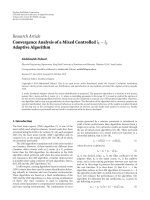
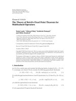
Figure 1: The MSE of the estimated channel versus SNR. The WP
algorithm.

15

20

25

30

SNR(2) = 10 dB
SNR(2) = 20 dB
SNR(2) = 30 dB

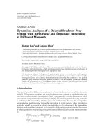
Figure 3: The MSE of the estimated channel versus SNR at the first
antenna for different values of SNR at the second antenna. The WP
algorithm.

10−2

100
10−1

10−3
MSE

MSE

10−2

10−4

10−3
10−4
10−5

10−5

50

100

150

200

250

10−6
−15

300

N

−5

0

5

10

15

20

25

30

SNR (dB)

Experimental
Analytical: (28)
Analytical: (32)

Experimental
Analytical: (48)
Analytical: (53)

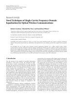
Figure 2: The MSE of the estimated channel versus number of data
samples. The WP algorithm.

(30) and (31) hold and
λmax Σ(1)
v

−10

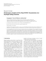
Figure 4: The MSE of the estimated channel versus SNR. The BP
algorithm.

5.
(1)

A(1) w1
1

2

.

(63)

Then, the MSE expressions (32) and (53) can be readily verified to coincide in the following two cases: when h(1) is es1
timated using the WP algorithm with both antennas, and
when h(1) is estimated using the BP algorithm with only the
1
first antenna.

SIMULATIONS

In this section, we validate our analytical results via computer
simulations. In all the examples, we consider K = 7 synchronous CDMA users that transmit BPSK-modulated symbols. Each point of the simulation curves is the result of averaging over 200 Monte-Carlo realizations of the noise and
transmission data sequences. In Figures 1–8, Gold codes of
length Lc = 31 are employed as the user spreading sequences


K. Zarifi and A. B. Gershman

9

10−2

102

100
10−2

MSE

MSE

10−3

10−4

10−4
10−6
10−8
10−10

10−5

50

100

150

200

250

10−12
−15

300

−10

−5

0

N

5

10

15

20

25

30

SNR (dB)
Σv
Σv
Σv
Σv
Σv
Σv

Σv

Experimental
Analytical: (48)
Analytical: (53)

Figure 5: The MSE of the estimated channel versus number of data
samples. The BP algorithm.

drawn randomly, q = 1
drawn randomly, q = 5
drawn randomly, q = 15
drawn according to (60)
drawn according to (61), q = 1
drawn according to (61), q = 5
drawn according to (61), q = 15

Figure 7: MSEs of the estimated channel versus SNR for eo = 28
and different matrices Σv . The BP algorithm.

102
100

100

MSE

10−2
10−1

10−4

10−2
MSE

10−6
10−8
10−10
10−12
−15

10−3
10−4

−10

−5

0

5

10

15

20

25

30

10−5

SNR (dB)
Uv drawn randomly
Uv drawn randomly
Uv drawn randomly

Uv drawn according to (57)
Uv drawn according to (59)

Figure 6: The MSE of the estimated channel versus SNR for Γv =
diag{20, 5, 3} and different matrices Uv . The BP algorithm.

and channel vectors of length L = 4 are independently drawn
from a zero-mean white complex Gaussian process and then
are scaled to become unit-norm vectors. The ambiguity in
the phase of the channel vector estimate is resolved by assuming that the phase of the first tap of the channel vector
is known at the receiver. In Figures 1–5 and 9, the received
noise at each antenna is considered to be a circular Gaussian
process such that [Σv ]i j , the (i, j)th entry of its covariance
matrix, is equal to 0.7|i− j | . In the figures where the MSE of

10−6
−15

−10

−5

0

5

10

15

20

25

30

SNR (dB)
LX algorithm
WP algorithm
BP algorithm

Figure 8: MSEs of the estimated channel versus SNR in the white
noise environment. The LX, WP, and BP algorithms.

the channel estimate is drawn versus SNR, it is assumed that
N = 80 data samples are used to estimate the channel.
Figures 1–3 illustrate the accuracy of our analytical results derived for the WP algorithm. In Figure 1, it is assumed
that SNRs of all users at both antennas are identical and h(1)
1
is estimated according to (22). The solid curve represents the

10

EURASIP Journal on Advances in Signal Processing
10−2

MSE

10−3

10−4

10−5

4

6

8
10
Channel length

Experimental, Lc = 40
Analytical: (48), Lc = 40
Analytical: (53), Lc = 40

12

14

Experimental, Lc = 80
Analytical: (48), Lc = 80
Analytical: (53), Lc = 80

Figure 9: MSEs of the estimated channel versus L for Lc = 40 and
Lc = 80. The BP algorithm.

MSE resulting from this estimate. This curve is compared
with our analytical results given by (28) and (32). It can be
observed that both theoretical curves follow the experimental MSE curve with a good precision. Note that when the SNR
is very low, the channel vector estimation error is quite large
and, hence, it could not be reliably predicted using the firstorder perturbation theory. In such a condition, the analytical
MSE curves obtained from (28) and (32) show a considerable
discrepancy with the experimental MSE curve.
Figure 2 depicts the experimental and the analytical MSE
curves versus the number of data samples N. In this figure,
it is assumed that the received signal power from each user
at each of the two antennas is equal to 10 dB. Due to the fact
that SNR is reasonably high, the theoretical curve (28) and
its high SNR approximation (32) are almost indistinguishable from each other and they follow the experimental MSE
curve with a good accuracy. It can be observed from Figure 2
that, when the number of data samples N is small, the small
perturbation assumption is violated, and, hence, the accuracy of the analytical MSE curves decreases.
Figure 3 shows the MSE of the estimated channel h(1) ver1
sus SNR at the first antenna (SNR(1) ) for 6 different values
of SNR at the second antenna (SNR(2) ). As expected from
Section 4.1, the performance of the channel estimation is
almost independent from the exact value of SNR(2) , unless
SNR(2) is very low.
Figures 4–7 and 9 show the performance of the BP algorithm and compare it to our analytical results. In Figure 4,

the experimental MSE curve is plotted versus SNR and is
compared with the theoretical curves obtained from (48) and
(53). As can be observed from the figure, the two theoretical MSE curves are very close to each other and also closely

follow the experimental MSE curve for the SNRs higher than
0 dB.
Figure 5 shows the experimental and the theoretical
curves drawn versus the number of data samples N for SNR
equal to 10 dB. As the figure shows, the theoretical curve (48)
is precisely followed by its high SNR approximation (53) and
both of them are very close to the experimental MSE curve.
Figure 6 shows the experimental MSE curves versus
SNR for noise covariance matrices with identical Γv =
diag{20, 5, 3} and different matrices of eigenvectors Uv .
Three random realizations of Uv as well as Uvmax and Uvmin
are drawn and then using (55) the corresponding noise covariance matrices are obtained. The BP algorithm is used
to estimate the channel vector in the presence of a correlated noise with the so-obtained noise covariance matrices.
Figure 6 confirms our theoretical results in Section 4.2 which
state that the worst and the best MSE performances are obtained when Uv = Uvmax and Uv = Uvmin , respectively. Note
that if Uv = Uvmin , then, unlike the MSE expression (53), the
experimental MSE performance is not equal to zero. It is due
to the fact that the MSE expression (53) is obtained using
the first-order perturbation theory and even in the high SNR
regime this expression has a slight difference with the experimental MSE.
Figure 7 plots the experimental MSE curves versus SNR
for noises with identical average energy of eo = Lc − L+1 = 28
and different covariance matrices. For each value of q = 1, 5,
and 15, one noise covariance matrix is drawn randomly and
another one is obtained according to (61). A rank-one noise
covariance matrix is also derived according to (60). Then,

the BP algorithm is used to estimate the channel vector in
the presence of correlated noise with the so-obtained noise
covariance matrices. Our analytical results in Section 4.2 are
validated by observing that the worst and the best MSE performances are obtained when the noise covariance matrix
follows (60) and (61), respectively.
In Figure 8, the performances of the LX, WP, and BP algorithms are tested in the white noise environment. As predicted by our analysis in Section 4, all three methods have a
nearly identical performance.
Figure 9 shows the experimental and the theoretical MSE
curves of the BP algorithm versus the channel length L for
two different values of the spreading factors Lc = 40 and Lc =
80. In this example, we use random spreading codes rather
than the optimized Gold codes. The entries of these codes are
randomly drawn from the set {−1, +1}. From Figure 9 we see
that, as predicted in Section 4, the estimation performance
decreases with increasing L. When Lc = 80, the MSE of the
channel vector estimate is significantly lower than that for
Lc = 40. It can be observed that the curves corresponding to
(48) and (53) are quite close to each other and, therefore, the
use of the random spreading codes instead of the Gold codes
retains the accuracy of (53).
6.

CONCLUSIONS

In this paper, analytical expressions for the MSE of the signature waveform estimation techniques of [15, 16] have been


K. Zarifi and A. B. Gershman

11

derived. Assuming that different user signature vectors are
orthogonal, the simplified versions of these expressions have
been also obtained for the high SNR regime. The effect of
the correlated noise on the performance of both algorithms
has been studied. It has been shown that the direction of the
eigenvectors of the noise covariance matrix has a significant
effect on the performance of both algorithms. In particular,
assuming that the eigenvalues of the noise covariance matrix are fixed, the noise covariance matrix eigenvectors corresponding to the extremal values of the MSEs have been
obtained. Over all noise covariance matrices with identical
average noise power, the extremal values of the MSEs have
been derived and it has been shown that both the maximal
and the minimal values of the MSEs are achieved when the
noise covariance matrix is rank deficient. Moreover, it has
been shown that at high SNRs and in the presence of white
noise, the performance of these two techniques is identical to
that of the conventional white noise-based technique of [9].
In the high SNR regime, it has been proved that the performance of the technique proposed in [15] is independent
from the noise covariance matrix and the user received power
at the second auxiliary antenna. This property has been generalized to the multiple antenna systems and it has been
shown that for such systems the choice of the auxiliary antenna is arbitrary at high SNRs.

2

δh(1)
1

E

(1) H

≈ w1

R(12)

†H

H

†

(1)
E δR(12) ΨδR(12) R(12) w1 .

(A.9)

Let us introduce
H

Ξ

E δR(12) ΨδR(12) .

(A.10)

From (A.2) and (A.3) it follows that
H

Ξ = E R(12) ΨR(12) .

(A.11)

Using (17) and (21) in (A.11) yields
Ξ=

1
N2

N

N

W(2) b( j) + v(2) ( j)

E
j =1 k=1

H

H

× b( j)H W(1) + v(1) ( j) Ψ
× W

(1)

(A.12)

(1)

b(k) + v (k)
H

H

× b(k)H W(2) + v(2) (k)

.

Using (A.2) to simplify the resulting expression, we obtain
1
Φ1 + Φ2 ,
N

Ξ=

(A.13)

where

APPENDICES
A.

Inserting (A.5) into (A.8) and applying the expectation operation to the squared norm of the resulting expression, we
have

PROOF OF THEOREM 1

Φ2

Since U(1) spans the null-space of R(12) , we have
n
H
U(1) W(1)
n

= 0.

ΨW

=W

( j)Ψv ( j)v
(1)

(2) H

H

Φ1 = E v(1) ( j)Ψv(1) ( j) W(2) W(2)
(1) H

H

Ψ = 0.

= E tr v(1) ( j)Ψv(1) ( j)

(A.2)

δR(12)

R(12) − R(12) ,

(A.3)

δU(1)
n

U(1) − U(1) .
n
n

(A.4)

Using the perturbation theory, the first-order approximation
of δU(1) can be written as [9, 26, 27]
n
≈ −R

(1) H

(12) †

H

δR

(12) H

U(1) ,
n

(A.5)

where
−1

†

( j) .

,

(A.14)

(A.1)

H

= tr E v(1) ( j)v(1) ( j)Ψ

To prove (28), we introduce

δU(1)
n

E v ( j)v
(2)

H

We also have

Equations (A.1) and (29) yield
(1)

H

E W(2) b( j)v(1) ( j)Ψv(1) ( j)bH ( j)W(2)

Φ1

H

R(12) = U(2) Ω(12) U(1) .
s
s
s

= tr Σ(1) Ψ W(2) W
v

Φ2 = E v

W(2) W(2)
W(2) W(2)

H
H

(A.15)

,
H

( j)Ψv ( j) E v(2) ( j)v(2) ( j)
(1)

= tr Σ(1) Ψ Σ(2) .
v
v

Substituting (A.15) into (A.13) and using (18), we obtain
1
(A.16)
tr Σ(1) Ψ R(2) .
v
N
Using (A.16) in (A.9) directly yields (28). To prove (32), first
we use (19) and (30) to obtain
Ξ=

(A.6)

Since

(1) H

(2) H

H

U(1) =
s

(1)
w(1)
w1
,..., K
(1)
(1)
w1
wK

,

Ω(12)
s
(1)H

Un C1 h(1) ≈ 0,
1

(A.7)

it follows that the first-order estimate of δh(1) is given by
1
(1) †

δh(1) ≈ −T1
1

H (1)
δU(1) w1 .
n

(A.8)

(1)

(2)

= diag A1 A1

(1)
w1

U(2) =
s

(2)
(1)
w1 , . . . , A(1) A(2) wK
K
K
(2)
w(2)
w1
,..., K

(2)
(2)
w1
wK

(2)
wK

,

.
(A.17)


12

EURASIP Journal on Advances in Signal Processing

Let

where
˘ (1)
w1

R

(12) †

(1)
w1

(12) −1

= U(2) Ωs
s

H (1)
U(1) w1 .
s

1

w(2) .
(1) (2)
(2) 2 1
A1 A1 w1

(A.19)

δh(1)
1

2

≈

Substituting R(2) from (18) into (A.20) and using (30) to simplify the result, we obtain
E

≈

NA(1)
1

1+

2

2

(2)
A(2) w1
1

4

.

(A.21)

(2)
As for any w1 and Σ(2) ,
v
H

2

(2)
(2)
(2)

w1 Σ(2) w1 ≤ w1 λmax Σ(2) ,
v
v

Lc −L+1 Lc −L+1

[Φ2 ]kl =

g =1

= E [v]m [v∗ ]k E [v]l [v]∗
g

Σv

lg

+ Σv

mg

Σv

ΨW = WH Ψ = 0.

Φ2

kl

=

g =1

H

H
≈ w1 R† E δ RH Ψδ R R† w1 ,

(B.3)

where
R − R.

Σv

= Σv ΨΣv

(B.2)

lk

ΨΣv

gk

+ ΨΣv

+ tr ΨΣv Σv

Φ2 = Σv ΨΣv

T

+ tr ΨΣv ΣT .
v

Us =

w
w1
,..., K
w1
wK

(B.5)

H

Ξ = E R ΨR .

(B.6)

Expanding the right-hand side of (B.6) according to (27),
and then using (B.2) to simplify the resulting expression, we
obtain
1
Ξ=
Φ1 + Φ2 ,
N

(B.7)

lk

(B.13)

(B.14)

,

Ωs = diag A2 w1 , . . . , A2 wK
K
1

Substituting (B.4) into (B.5), and then using (B.2) to simplify
the result, we have

Σv

lk .

2

E δ RH Ψδ R .

gg

Substituting (B.10) and (B.14) into (B.7) and using the resulting expression in (B.3), we obtain (48).
To prove (53), we note that (13) along with (24) yield

(B.4)

Let us denote

lg

From (B.13) it directly follows that

Using the procedure similar to that in Appendix A, it can be
readily shown that

Ξ

lk .

Lc −L+1

(B.1)

From (51) along with (B.1) it follows that

δR

mk

Substituting (B.12) into (B.11), we obtain

UH W = 0.
n

2

(B.12)

+ E [v]m [v]∗ E [v]l [v]∗
g
k
= Σv

According to (24), we have

δh1

[Ψ]gm E [v]∗ [v]∗ [v]m [v]l , (B.11)
g
k

E [v]∗ [v]∗ [v]m [v]l
g
k

(A.22)

PROOF OF THEOREM 2

E

m=1

where [·]k is the kth entry of a vector and the time index i
has been dropped from v(i) for the sake of simplicity. Since

v is a multivariate circular Gaussian random vector, we have
[28]

then, when (31) holds, (32) directly follows from (A.21). This
completes the proof.
B.

(B.10)

where the second line of (B.10) can be derived using the same
steps as in (A.15). To obtain Φ2 , it can be easily shown from
(B.9) that

H

(2)
(2)
w1 Σ(2) w1
v

(B.8)
(B.9)

= tr Σv Ψ W∗ WT ,

H
tr Σ(1) Ψ
(2)
v
w(2) R(2) w1 .

(1) 2 (2) 2
(2) 4 1
NA1 A1 w1

tr Σ(1) Ψ
v

E v (i)v (i)Ψv(i)v (i) ,

Φ1 = E vH (i)Ψv(i) W∗ WT ,

(A.20)

2
δh(1)
1

T

and (·)∗ stands for the conjugate. Since the transmitted symbols are drawn from the BPSK constellation, we have

Using (A.19) along with (28) yields
E

H

∗

Φ2

Substituting (A.17) into (A.18) and using (30), we have
˘ (1)
w1 =

E vH (i)Ψv(i)W∗ b(i)bT (i)WT ,

Φ1

(A.18)

Vs =

∗

∗

w
w1
,..., K
w1
wK

2

,

(B.15)

.

Let us denote
˘
w1

−1

R† w1 = Vs Ωs UH w1 .
s

(B.16)

Substituting (B.15) into the right-hand side of (B.16) and using (13), we have
˘
w1 =

∗
w1
A2 w1
1

2.

(B.17)


K. Zarifi and A. B. Gershman

13

Using (B.17) in (48) results in the following expression for

E{ δh1 2 }:
δh1

E

2

≈

tr ΨΣv
α1 + α2 + α3 ,
2
N w1 A4
1

(B.18)

where
T
w1
w∗
W∗ WT 1 ,
w1
w1

α1
α2

T
∗

w1 T w1
Σv
,
w1
w1
T
w1
w1

1
tr ΨΣv

α3

Σv ΨΣv

(B.19)
T

∗
w1
.
w1

It directly follows from (13) that
2

α1 = A2 w1 .
1

(B.20)

Noting that both Σv and Ψ are positive (semi-) definite matrices, it is easy to find an upper-bound for α2 and α3 as
α2 =

H
w1
w
Σv 1
w1
w1

1
α3 =
tr ΨΣv

∗

≤ λ∗ Σv = λmax Σv ,
max

H
w1
w1

Σv ΨΣv

w1
w1

≤

1
λ∗ Σv ΨΣv
max
tr ΨΣv

=

1
λmax Σv ΨΣv
tr ΨΣv

≤

∗

λmax ΨΣv
λmax Σv ≤ λmax Σv .
tr ΨΣv

(B.21)

Hence, if (52) holds, both α2 and α3 are negligible comparing
to α1 . Substituting (B.20) into (B.18) directly yields (53). This
completes the proof.
ACKNOWLEDGMENTS
This work was supported by the Wolfgang Paul Award Program of the Alexander von Humboldt Foundation and German Ministry of Education and Research.
REFERENCES
´

[1] S. Verdu, Multiuser Detection, Cambridge University Press,
Cambridge, UK, 1998.
[2] M. Honig, U. Madhow, and S. Verdu, “Blind adaptive multiuser detection,” IEEE Transactions on Information Theory,
vol. 41, no. 4, pp. 944–960, 1995.
[3] X. Wang and H. V. Poor, “Blind multiuser detection: a subspace approach,” IEEE Transactions on Information Theory,
vol. 44, no. 2, pp. 677–690, 1998.
[4] Z. Xu, P. Liu, and X. Wang, “Blind multiuser detection: from
MOE to subspace methods,” IEEE Transactions on Signal Processing, vol. 52, no. 2, pp. 510–524, 2004.

[5] K. Zarifi, S. Shahbazpanahi, A. B. Gershman, and Z.-Q. Luo,
“Robust blind multiuser detection based on the worst-case
performance optimization of the MMSE receiver,” IEEE Transactions on Signal Processing, vol. 53, no. 1, pp. 295–305, 2005.
[6] U. Madhow and M. L. Honig, “MMSE interference suppression for direct-sequence spread-spectrum CDMA,” IEEE
Transactions on Communications, vol. 42, no. 12, pp. 3178–
3188, 1994.
[7] U. Mitra and H. V. Poor, “Adaptive receiver algorithms for
near-far resistant CDMA,” IEEE Transactions on Communications, vol. 43, no. 2–4, part 3, pp. 1713–1724, 1995.
[8] S. E. Bensley and B. Aazhang, “Subspace-based channel estimation for code division multiple access communication systems,” IEEE Transactions on Communications, vol. 44, no. 8,
pp. 1009–1020, 1996.
[9] H. Liu and G. Xu, “Subspace method for signature waveform
estimation in synchronous CDMA systems,” IEEE Transactions
on Communications, vol. 44, no. 10, pp. 1346–1354, 1996.
[10] M. Torlak and G. Xu, “Blind multiuser channel estimation in
asynchronous CDMA systems,” IEEE Transactions on Signal
Processing, vol. 45, no. 1, pp. 137–147, 1997.
[11] X. Wang and H. V. Poor, “Blind equalization and multiuser
detection in dispersive CDMA channels,” IEEE Transactions on
Communications, vol. 46, no. 1, pp. 91–103, 1998.
[12] Z. Xu and M. K. Tsatsanis, “Blind adaptive algorithms for minimum variance CDMA receivers,” IEEE Transactions on Communications, vol. 49, no. 1, pp. 180–194, 2001.
[13] Q. Li, C. N. Georghiades, and X. Wang, “Blind multiuser detection in uplink CDMA with multipath fading: a sequential

EM approach,” IEEE Transactions on Communications, vol. 52,
no. 1, pp. 71–81, 2004.
[14] S. Buzzi, M. Lops, and H. V. Poor, “Code-aided interference
suppression for DS/CDMA overlay systems,” Proceedings of the
IEEE, vol. 90, no. 3, pp. 394–435, 2002.
[15] X. Wang and H. V. Poor, “Blind joint equalization and multiuser detection for DS-CDMA in unknown correlated noise,”
IEEE Transactions on Circuits and Systems for Video Technology
II, vol. 46, no. 7, pp. 886–895, 1999.
[16] S. Buzzi and H. V. Poor, “A single-antenna blind receiver
for multiuser detection in unknown correlated noise,” IEEE
Transactions on Vehicular Technology, vol. 51, no. 1, pp. 209–
215, 2002.
[17] N. Yuen and B. Friedlander, “Asymptotic performance analysis for signature waveform estimation in synchronous CDMA
systems,” IEEE Transactions on Signal Processing, vol. 46, no. 6,
pp. 1753–1757, 1998.
[18] Z. Xu, “On the second-order statistics of the weighted sample covariance matrix,” IEEE Transactions on Signal Processing,
vol. 51, no. 2, pp. 527–534, 2003.
[19] Z. Xu, “Effects of imperfect blind channel estimation on performance of linear CDMA receivers,” IEEE Transactions on Signal Processing, vol. 52, no. 10, part 1, pp. 2873–2884, 2004.
[20] K. Zarifi and A. B. Gershman, “Performance analysis of
subspace-based signature waveform estimation algorithms for
DS-CDMA systems with unknown correlated noise,” in Proceedings of 6th IEEE Workshop on Signal Processing Advances
in Wireless Communications (SPAWC ’05), pp. 600–604, New
York, NY, USA, June 2005.
[21] A. Høst-Madsen, X. Wang, and S. Bahng, “Asymptotic analysis
of blind multiuser detection with blind channel estimation,”
IEEE Transactions on Signal Processing, vol. 52, no. 6, pp. 1722–
1738, 2004.


14

[22] M. Honig and M. K. Tsatsanis, “Adaptive techniques for multiuser CDMA receivers,” IEEE Signal Processing Magazine,
vol. 17, no. 3, pp. 49–61, 2000.
[23] S. Parkvall, “Variability of user performance in cellular DSCDMA-long versus short spreading sequences,” IEEE Transactions on Communications, vol. 48, no. 7, pp. 1178–1187, 2000.
[24] I. D. Coope and P. F. Renaud, “Trace inequalities with applications to orthogonal regression and matrix nearness problems,” Report UCDMS2000/17, Department of Mathematics
and Statistics, University of Canterbury, Christchurch, New
Zealand, November 2000, />research/ucdms2000n17.pdf.
[25] R. A. Horn and C. R. Johnson, Matrix Analysis, Cambridge
University Press, Cambridge, UK, 1999.
[26] F. Li, H. Liu, and R. J. Vaccaro, “Performance analysis for DOA
estimation algorithms: unification, simplification, and observations,” IEEE Transactions on Aerospace and Electronic Systems, vol. 29, no. 4, pp. 1170–1184, 1993.
[27] Z. Xu, “Perturbation analysis for subspace decomposition with
applications in subspace-based algorithms,” IEEE Transactions
on Signal Processing, vol. 50, no. 11, pp. 2820–2830, 2002.
[28] D. R. Brillinger, Time Series: Data Analysis and Theory, vol. 36
of Classics in Applied Mathematics, SIAM, Philadelphia, Pa,
USA, 2001.
Keyvan Zarifi received his B.S. and M.S.
degrees both in electrical engineering from
University of Tehran, Tehran, Iran, in 1997
and 2000, respectively. From January 2002
until March 2005, he was with the Department of Communication Systems, University of Duisburg-Essen, Duisburg, Germany. From April 2005, he has been with
the Department of Communication Systems, Darmstadt University of Technology,
Darmstadt, Germany, where he currently pursues his Ph.D. From
September 2002 until March 2003, he was a Visiting Scholar at the
Department of Electrical and Computer Engineering, McMaster
University, Hamilton, Ontario, Canada. His research interests include statistical signal processing, multiuser detection, blind estimation techniques, and MIMO communications.
Alex B. Gershman received his Diploma
and Ph.D. degrees in radiophysics and electronics from the Nizhny Novgorod State
University, Russia, in 1984 and 1990, respectively. From 1984 to 1999, he held several full-time and visiting research appointments in Russia, Switzerland, and Germany.
In 1999, he joined the Department of Electrical and Computer Engineering, McMaster University, Hamilton, Ontario, Canada,

where he became a Full Professor in 2002. From April 2005, he
has been with the Darmstadt University of Technology, Darmstadt,
Germany, as a Professor and Head of the Communication Systems Group. His research interests span the areas of signal processing and communications with primary emphasis on statistical signal and array processing, adaptive beamforming, MIMO and
space-time communications, multiuser and multicarrier communications, radar and sonar signal processing, and estimation and
detection theory. He received the 2004 IEEE Signal Processing Society Best Paper Award. He is a Fellow of the IEEE and a recipient of
the 2001 Wolfgang Paul Award from the Alexander von Humboldt

EURASIP Journal on Advances in Signal Processing
Foundation, Germany, the 2002 Young Explorers Prize from the
Canadian Institute for Advanced Research (CIAR), and the 2000
Premier’s Research Excellence Award, Ontario, Canada. He is currently Editor-in-Chief of the IEEE Signal Processing Letters. He
was Associate Editor of the IEEE Transactions on Signal Processing (1999–2006). He is on Editorial Boards of EURASIP Journal
on Wireless Communications and Networking and EURASIP Signal Processing Journal. He is Vice-Chair of the Sensor Array and
Multichannel (SAM) Technical Committee (TC) of the IEEE Signal
Processing Society.