Báo cáo hóa học: " A Generalized Algorithm for the Generation of Correlated Rayleigh Fading Envelopes in Wireless Channels" ppt
Bạn đang xem bản rút gọn của tài liệu. Xem và tải ngay bản đầy đủ của tài liệu tại đây (1012.82 KB, 15 trang )
EURASIP Journal on Wireless Communications and Networking 2005:5, 801–815
c
2005 Le Chung Tran et al.
A Generalized Algorithm for the Generation
of Correlated Rayleigh Fading Envelopes
in Wireless Channels
Le Chung T ran
Telecommunications and Information Technology Research Institute (TITR), School of Electrical, Computer and Telecommunications
Engineer ing, University of Wollongong, Wollongong NSW 2522, Australia
Email:
Tadeusz A. Wysocki
School of Electrical Computer and Telecommunications Engineering, Faculty of Informatic s, University of Wollongong,
Wollongong NSW 2522, Australia
Email:
Alfred Mertins
Signal Processing Group, Department of Physics, Universit y of Oldenburg, 26111 Oldenburg, Germany
Email:
Jennifer Seberry
School of Information Technology and Computer Science, Faculty of Informatics, University of Wollongong,
Wollongong NSW 2522, Australia
Email:
Received 23 January 2005; Revised 6 July 2005; Recommended for Publication by Wei Li
Although generation of correlated Rayleigh fading envelopes has been intensively considered in the literature, all conventional
methods have their own shortcomings, which seriously impede their applicability. A very general, straightforward algorithm for
the generation of an arbit rary number of Rayleigh envelopes with any desired, equal or unequal power, in wireless channels either
with or without Doppler frequency shifts, is proposed. The proposed algorithm can be applied to the case of spat ial correlation, such
as with multiple antennas in multiple-input multiple-output (MIMO) systems, or spectral correlation between the random pro-
cesses like in orthogonal frequency-division multiplexing (OFDM) systems. It can also be used for generating correlated Rayleigh
fading envelopes in either discrete-time instants or a real-time scenario. Besides being more generalized, our proposed algorithm is
more precise, while overcoming all shortcomings of the conventional methods.
Keywords and phrases: correlated Rayleigh fading envelopes, antenna ar rays, OFDM, MIMO, Doppler frequency shift.
1. INTRODUCTION
In orthogonal frequency-division multiplexing (OFDM) sys-
tems, the fading affecting carriers may have cross-correlation
due to the small coherence bandwidth of the channel, or due
to the inadequate frequency separation between the carriers.
In addition, in multiple-input multiple-output (MIMO) sys-
tems where multiple antennas are used to transmit and/or
This is an open access article distributed under the Creative Commons
Attribution License, which permits unrestricted use, distr ibution, and
reproduction in any medium, provided the original work is properly cited.
receive signals, the fading affecting these antennas may also
experience cross-correlation due to the inadequate separa-
tion between the antennas. Therefore, a generalized, straight-
forward and, certainly, correct algorithm to generate corre-
lated Rayleigh fading envelopes is required for the researchers
wishing to analyze theoretically and simulate the perfor-
mance of systems.
Because of that, generation of correlated Rayleigh fading
envelopes has been intensively mentioned in the literature,
such as [1, 2, 3, 4, 5, 6, 7, 8, 9, 10, 11, 12, 13]. However, be-
sides not being adequately generalized to be able to apply to
various scenarios, all conventional methods have their own
802 EURASIP Journal on Wireless Communications and Networking
shortcomings which seriously limit their applicability or even
cause failures in generating the desired Rayleigh fading en-
velopes.
In this paper, we modify existing methods and propose a
generalized algor ithm for generating correlated Rayleigh fad-
ing envelopes. Our modifications are simple,butimportant
and also ver y efficient. The proposed algorithm thus incor-
porates the advantages of the existing methods, while over-
coming all of their shortcomings. Furthermore, besides being
more generalized, the proposed algorithm is more accurate,
while providing more useful features than the conventional
methods.
The paper is organized as follows. In Section 2,asum-
mary of the shortcomings of conventional methods for gen-
erating correlated Rayleigh fading envelopes is derived. In
Sections 3.1 and 3.2, we shortly review the discussions on
the correlation property between the transmitted sig nals as
functions of time delay and frequency separation, such as in
OFDM systems, and as functions of spatial separation be-
tween transmission antennas, such as in MIMO systems, re-
spectively. In Section 4, we propose a very general, straight-
forward algorithm to generate correlated Rayleigh fading en-
velopes. Section 5 derives an algorithm to generate correlated
Rayleigh fading envelopes in a real-time scenario. Simulation
results are presented in Section 6.Thepaperisconcludedby
Section 7.
2. SHORTCOMINGS OF CONVENTIONAL METHODS
AND AIMS OF THE PROPOSED ALGORITHM
We first analyze the shortcomings of some conventional
methods for the generation of correlated Rayleigh fading en-
velopes.
In [3], the authors derived fading correlation proper-
ties in antenna arrays and, then, briefly mentioned the algo-
rithm to generate complex Gaussian random variables (with
Rayleigh envelopes) corresponding to a desired correlation
coefficient matrix. This algorithm was proposed for gener-
ating equal power Rayleigh envelopes only, rather than arbi-
trary (equal or unequal) power Rayleigh envelopes.
In [4, 5], the authors proposed different methods for
generating only N = 2 equal power correlated Rayleigh en-
velopes. In [6], the authors generalized the method of [5]for
N ≥ 2. However, in this method, Cholesky decomposition
[7] is used, and consequently, the covariance matrix must be
positive definite, which is not always realistic. An example,
where the covariance matrix is not positive definite, is de-
rived later in Example 1 of Section 4.1 of this paper.
These methods were then more generalized in [8], where
one can generate any number of Rayleigh envelopes corre-
sponding to a desired covariance matrix and with any power,
that is, even with unequal po wer. However, again, the covari-
ance matrix must be positive definite in order for Cholesky
decomposition to be performable. In addition, the authors in
[8] forced the covariances of the complex Gaussian random
variables (with Rayleigh fading envelopes) to be real (see [8,
(8)]). This limitation prohibits the use of their method in
various cases because, in fact, the covariances of the com-
plex Gaussian random variables are more likely to be com-
plex.
In [2], the authors proposed a method for generating
any number of Rayleigh envelopes with equal power only. Al-
though the method of [2] works well in various cases, it fails
to perform Cholesky decomposition for some complex co-
variance matrices in Matlab due to the roundoff errors of
Matlab.
1
This shortcoming is overcome by some modifica-
tions mentioned later in our proposed algorithm.
More importantly, the method proposed in [2] fails to
generate Rayleigh fading envelopes corresponding to a de-
sired covariance matrix in a real-time scenario where Doppler
frequency shifts are considered. This is because passing Gaus-
sian random variables with variances assumed to b e equal
to one (for simplicity of explanation) through a Doppler fil-
ter changes remarkably the variances of those variables. The
variances of the variables at the outputs of Doppler filters are
not equal to one any more, but depend on the variance of the
variables at the inputs of the filters as well as the character-
istics of those filters. The authors in [2] did not realize this
variance-changing effect caused by Doppler filters. We will
return to this issue later in this paper.
For the aforementioned reasons, a more generalized algo-
rithm is required to generate any number of Rayleigh fading
envelopes with any power (equal or unequal power) corre-
sponding to any desired covariance matrix. The algorithm
should be applicable to both discrete time instant scenario
and real-time scenario. The algorithm is also expected to
overcome roundoff errors which may cause the interrup-
tion of Matlab programs. In addition, the algorithm should
work well, regardless of the positive definiteness of the co-
variance matrices. Furthermore, the algorithm should pro-
vide a straightforward method for the generation of com-
plex Gaussian random variables (with Rayleigh envelopes)
with correlation properties as functions of time delay and
frequency separation (such as in OFDM systems), or spatial
separation between transmission antennas (like with multi-
ple antennas in MIMO systems). This paper proposes such
an algorithm.
3. BRIEF REVIEW OF STUDIES ON FADING
CORRELATION CHARACTERISTICS
In this section, we shortly review the discussions on the cor-
relation property between the transmitted signals as func-
1
It has been well known that Cholesky decomposition may not work for
the matrix having eigenvalues being equal or close to zeros. We consider the
following covariance matrix K, for instance:
K
=
1.04361 0.7596 −0.3840i 0.6082 −0.4427 i 0.4085 −0 .8547i
0.7596 +0.3840i 1.04361 0.7780 −0.3654i 0.6082 −0.4427i
0.6082 +0.4427i 0.7780 +0.3654i 1.04361 0.7596 −0.3840i
0.4085 +0.8547i 0.6082 +0.4427i 0.7596 + 0.3840i 1.04361
.
Cholesky decomposition does not work for this covariance matrix although
it is positive definite.
Algorithm for Generating Correlated Rayleigh Envelopes 803
tions of time delay and frequency separation, such as in
OFDM systems, and as functions of spatial separation be-
tween transmission antennas, such as in MIMO systems.
These discussions were originally derived in [3, 9], respec-
tively.
This review aims at facilitating readers to apply our pro-
posed algorithm in different scenarios (i.e., spectral correla-
tion, such as in OFDM systems, or spatial correlation,such
as in MIMO systems) as well as pointing out the condition
for the analyses in [3, 9]tobeapplicabletoourproposedal-
gorithm (i.e., these analyses are applicable to our algorithm
if the powers (variances) of different random processes are
assumed to be the same).
3.1. Fading correlation as functions of time delay and
frequency separation
In [9], Jakes considered the scenario where all complex Gaus-
sian random processes with Rayleigh envelopes have equal
powers σ
2
and derived the correlation properties between
random processes as functions of both time delay and fre-
quency separation, such as in OFDM systems. Let z
k
(t)and
z
j
(t) be the two zero-mean complex Gaussian random pro-
cesses at time instant t, corresponding to frequencies f
k
and
f
j
,respectively.Denote
x
k
Re
z
k
(t)
, y
k
Im
z
k
(t)
,
x
j
Re
z
j
t + τ
k, j
, y
j
Im
z
j
t + τ
k, j
,
(1)
where τ
k, j
is the arrival time delay between two signals and
Re(·), Im(·) are the real and imaginar y parts of the argu-
ment, respectively. By definition, the covariances between the
real and imaginary parts of z
k
(t)andz
j
(t + τ
k, j
)are
R
xx
k, j
E
x
k
x
j
, R
yy
k, j
E
y
k
y
j
,
R
xy
k, j
E
x
k
y
j
, R
yx
k, j
E
y
k
x
j
.
(2)
Then, those covariances have been derived in [9, (1.5-20)] as
R
xx
k, j
= R
yy
k, j
=
σ
2
J
0
2πF
m
τ
k, j
2
1+
∆ω
k, j
σ
τ
2
,
R
xy
k, j
=−R
yx
k, j
=−∆ω
k, j
σ
τ
R
xx
k, j
,
(3)
where σ
2
is the variance (power) of the complex Gaussian
random processes (σ
2
/2 is the variance per dimension); J
0
is the first-kind Bessel function of the zeroth-order; F
m
is
the maximum Doppler frequency F
m
= v/λ = vf
c
/c.In
this formula, λ is the wavelength of the carrier, f
c
is the car-
rier frequency, c is the speed of light, and v is the mobile
speed; ∆ω
k, j
= 2π( f
k
− f
j
) is the angular frequency sep-
aration between the two complex Gaussian processes with
Rayleigh envelopes at frequencies f
k
and f
j
; σ
τ
is the root-
mean-square (rms) delay spread of the wireless channel.
∆
∆
Receiver
Φ
K
Transmit antennas
T
x−1
T
x
D
12
Figure 1: Model to examine the spatial correlation between trans-
mitter antennas.
It should be emphasized that, the equalities (3)holdonly
when the set of multipath channel coefficients, which were de-
noted as C
nm
and derived in [9, (1.5-1) and (1.5-2)], as well as
the powers are assumed to be the same for different random
processes (with different frequencies). Readers may refer to
[9, pages 46–49] for an explicit exposition.
3.2. Fading correlation as functions of spatial
separation in antenna arrays
The fading correlation properties between wireless channels
as functions of antenna spacing in multiple antenna sys-
tems have been mentioned in [3]. Figure 1 presents a typ-
ical model of the channel where all signals from a receiver
are assumed to arrive at T
x
antennas within ±∆ at angle Φ
(|Φ|≤π). Let λ be the wavelength, D the distance between
the two adjacent transmitter antennas, and z = 2π(D/λ).
In [3], it is assumed that fading corresponding to different
receivers is independent. This is reasonable if receivers are
not on top of each other within some wavelengths and they
are surrounded by their own scatterers. Consequently, we
only need to calculate the correlation properties for a typi-
cal receiver. The fading in the channel between a given kth
transmitter antenna and the receiver may be considered as
a zero-mean, complex Gaussian random variable, which is
presented as b
(k)
= x
(k)
+ iy
(k)
. Denote the covariances be-
tween the real parts as well as the imaginary parts them-
selves of the fading corresponding to the kth and jth trans-
mitter antennas
2
to be R
xx
k, j
and R
yy
k, j
, while those terms
between the real and imaginary parts of the fading to be
R
xy
k, j
and R
yx
k, j
. The terms R
xx
k, j
, R
yy
k, j
, R
xy
k, j
,andR
yx
k, j
are similarly defined as (2). Then, it has been proved that the
closed-form expressions of these covariances normalized by
the variance per dimension (real and imaginary) are (see [3,
2
Note that k and j here are antenna indices, while they are frequency
indices in Section 3.1.
804 EURASIP Journal on Wireless Communications and Networking
(A. 19) and (A. 20)])
˜
R
xx
k, j
=
˜
R
yy
k, j
=J
0
z(k−j)
+2
∞
m=1
J
2m
z(k−j)
cos(2mΦ)
sin(2m∆)
2m∆
,
(4)
˜
R
xy
k, j
=−
˜
R
yx
k, j
= 2
∞
m=0
J
2m+1
z(k − j)
sin
(2m +1)Φ
×
sin
(2m +1)∆
(2m +1)∆
,
(5)
where
˜
R
k, j
= 2R
k, j
/σ
2
. In other words, we have
R
k, j
=
σ
2
˜
R
k, j
2
. (6)
In these equations, J
q
is the first-kind Bessel function of the
integer order q,andσ
2
/2 is the variance per dimension of
the received signal at each transmitter antenna, that is, it is
assumed in [3] that the signals corresponding to different
transmitter antennas have equal variances σ
2
.
Similarly to Section 3.1, the equalities (4)and(5)hold
only when the set of multipath channel coefficients,which
were denoted as g
n
and derived in [3, (A-1)], and the powers
are assumed to be the same for different random processes.
Readers may refer to [3, pages 1054–1056] for an explicit ex-
position.
4. GENERALIZED ALGORITHM TO GENERATE
CORRELATED, FLAT RAYLEIGH FADING ENVELOPES
4.1. Covariance matrix of complex Gaussian random
variables with Rayleigh fading envelopes
It is known that Rayleigh fading envelopes can be gener-
ated from zero-mean, complex Gaussian random variables.
We consider here a column vector Z of N zero-mean, com-
plex Gaussian random variables with variances (or powers)
σ
g
2
j
,forj = 1, , N.DenoteZ = (z
1
, , z
N
)
T
,wherez
j
( j = 1, , N)isregardedas
z
j
= r
j
e
iθ
j
= x
j
+ iy
j
. (7)
The modulus of z
j
is r
j
=
x
2
j
+ y
2
j
. It is assumed that
the phases θ
j
’s are independent, identically uniformly dis-
tributed random variables. As a result, the real and imaginary
parts of each z
j
are independent (but z
j
’s are not necessarily
independent), that is, the covariances E(x
j
y
j
) = 0forforall
j and therefore, r
j
’s are Rayleigh envelopes.
Let σ
2
g
xj
and σ
2
g
yj
be the variances per dimension (real and
imaginary), that is, σ
2
g
xj
=E(x
2
j
), σ
2
gyj
=E(y
2
j
). Clearly, σ
2
g
j
=σ
2
g
xj
+
σ
2
g
yj
.Ifσ
2
g
xj
=σ
2
g
yj
, then σ
2
g
xj
=σ
2
g
yj
= σ
2
g
j
/2. Note that we consider
a very general scenario where the variances (powers) of the
real parts are not necessarily equal to those of the imaginary
parts. Also, the powers of Rayleigh envelopes denoted as σ
2
r
j
are not necessarily equal to one another. Therefore, the sce-
nario where the variances of the Rayleigh envelopes are equal
to one another and the powers of real parts are equal to those
of imaginary parts, such as the scenario mentioned in either
Section 3.1 or Section 3.2, is considered as a particular case.
For k = j, we define the covariances R
xx
k, j
, R
yy
k, j
, R
xy
k, j
,
and R
yx
k, j
between the real as well as imaginary parts of z
k
and z
j
, similarly to those mentioned in (2).
By definition, the covariance matrix K of Z is
K = E
ZZ
H
µ
k, j
N×N
,(8)
where (·)
H
denotes the Hermitian transposition operation
and
µ
k, j
=
σ
2
g
j
if k ≡ j,
R
xx
k, j
+ R
yy
k, j
− i
R
xy
k, j
− R
yx
k, j
if k = j.
(9)
In reality, the covariance matrix K is not always positive
semidefinite. An example where the covariance matrix K is
not positive semidefinite is derived as follows.
Example 1. We examine an antenna array comprising 3
transmitter antennas. Let D
kj
,fork, j = 1, , 3, be the dis-
tance between the kth antenna and the jth antenna. The dis-
tance D
jk
between jth antenna and the kth antenna is then
D
jk
=−D
kj
. Specifically, we consider the case
D
21
= 0.0385λ,
D
31
= 0.1789λ,
D
32
= 0.1560λ,
(10)
where λ is the wavelength. Clearly, these antennas are neither
equally spaced, nor positioned in a straight line. Instead, they
are positioned at the 3 peaks of a triangle.
If the receiver antenna is far enough f rom the transmit-
ter antennas, we can assume that all signals from the receiver
arrive at the transmitter antennas within
±∆ at angle Φ (see
Figure 1 for the illustration of these notations). As a result,
the analytical results mentioned in Section 3.2 with small
modifications can still be applied to this case. In particular,
covariance matrix K can still be calculated following (4), (5),
(6), (8), and (9), provided that, in (4)and(5), the products
z(k − j)(or2πD(k − j)/λ) are replaced by 2πD
kj
/λ. This is
because, in our considered case, D
kj
are the actual distances
between the kth transmitter antenna and the jth transmitter
antenna, for k, j = 1, ,3.
Further, we assume that the variance σ
2
of the received
signals at each transmitter antenna in (6) is unit, that is, σ
2
=
1. We also assume that Φ = 0.1114π rad and ∆ = 0.1114π
rad.
Algorithm for Generating Correlated Rayleigh Envelopes 805
In order to examine the performance of the considered
system, the Rayleigh fading envelopes are required to be sim-
ulated. In turn, the covariance matrix of the complex Gaus-
sian random variables corresponding to these Rayleigh en-
velopes must be calculated. Based on the aforementioned as-
sumptions, from the theoretically analytical equations (4),
(5), and (6), and the definition equations (8)and(9), we have
the following desired covariance matrix for the considered
configuration of transmitter antennas:
K =
1.0000 0.9957 + 0.0811i 0.9090 + 0.3607i
0.9957−0.0811i 1.0000 0.9303 + 0.3180i
0.9090−0.3607i 0.9303−0.3180i 1.0000
.
(11)
Performing eigen decomposition, we have the following
eigenvalues: −0.0092; 0.0360; and 2.9733. Therefore, K is not
positive semidefinite. This also means that K is not positive
definite.
It is important to emphasize that, from the mathemat-
ical point of view, covariance matrices are always positive
semidefinite by definition (8), that is, the eigenvalues of the
covariance matrices are either zero or positive. However, this
does not contradict the above example where the covariance
matrix K has a negative eigenvalue. The main reason why
the desired covariance matrix K is not positive semidefinite
is due to the approximation and the simplifications of the
model mentioned in Figure 1 in calculating the covariance
values, that is, due to the preciseness of (4)and(5), com-
pared to the true covariance values. In other words, errors
in estimating covariance values may exist in the calculation.
Those errors may result in a covariance matrix being not pos-
itive semidefinite.
A question that could be raised here is why the covari-
ance matrix of complex Gaussian random variables (with
Rayleigh fading envelopes), rather than the covariance ma-
trix of Rayleigh envelopes, is of particular interest. This is due
to the two following reasons.
From the physical point of view, in the covariance ma-
trix of Rayleigh envelopes, the correlation properties R
xx
, R
yy
of the real components (inphase components) as well as
the imaginary components (quadrature phase components)
themselves and the correlation properties R
xy
, R
yx
between
the real and imaginary components of random variables are
not directly present (these correlation properties are defined
in (2)). On the contrar y, those correlation properties are
clearly present in the covariance matrix of complex Gaus-
sian random variables with the desired Rayleigh envelopes.
In other words, the physical significance of the correlation
properties of random variables is not present as detailed in
the covariance matrix of Rayleigh envelopes as in the covari-
ance matrix of complex Gaussian random variables with the
desired Rayleigh envelopes.
Further, from the mathematical point of view, it is pos-
sible to have one-to-one mapping from the cross-correlation
coefficients ρ
gij
(between the ith and jth complex Gaussian
random variables) to the cross-correlation coefficients ρ
rij
(between Rayleigh fading envelopes) as follows (see [9, (1.5-
26)]):
ρ
rij
=
1+
ρ
gij
E
int
2
ρ
gij
/
1+
ρ
gij
− π/2
2 − π/2
, (12)
where E
int
(·) is the complete elliptic integral of the second
kind. Some good approximations of this relationship be-
tween ρ
rij
and ρ
gij
are presented in the mapping [4,Table
II], the look-up [8,TableIandFigure1].
However, the reversed mapping, that is, the mapping
from ρ
rij
to ρ
gij
,ismultivalent. It means that, for a given
ρ
rij
, we have to somehow determine ρ
gij
in order to gener-
ate Rayleigh fading envelopes and the possible values of ρ
gij
may be significantly different from each other depending on
how ρ
gij
is determined from ρ
rij
. It is noted that ρ
rij
is always
real, but ρ
gij
may be complex.
For the two aforementioned reasons, the covariance ma-
trix of complex Gaussian random variables (with Rayleigh
envelopes), as opposed to the covariance matrix of Rayleigh
envelopes, is of particular interest in this paper.
4.2. Forced positive semidefiniteness
of the covariance matrix
First, we need to define the coloring matrix L corresponding
to a covariance matrix K .Thecoloring matrix L is defined
to be the N × N matrix satisfying
LL
H
= K. (13)
It is noted that the coloring matrix is not necessarily a lower
triangular matrix. Particularly, to determine the coloring ma-
trix L corresponding to a covariance matrix K,wecanuse
either Cholesky decomposition [7]asmentionedinanum-
ber of papers, which have been reviewed in Section 2 of this
paper, or eigen decomposition which is mentioned in the
next section of this paper. The former yields a lower trian-
gular coloring matrix, while the later yields a square coloring
matrix.
Unlike Cholesky decomposition, where the covariance
matrix K mu st be positive definite, eigen decomposition re-
quires that K is at least positive semidefinite, that is, the eigen-
values of K are either zeros or positive. We wil l explain later
why the covariance matrix must be positive semidefinite even
in the case where eigen decomposition is used to calculate the
coloring matrix. The covariance matrix K, in fact, may not
be positive semidefinite, that is, K may have negative eigen-
values, as the case mentioned in Example 1 of Section 4.1.
To overcome this obstacle, similarly to (but not exactly
as) the method in [2], we approximate the given covariance
matrix by a matrix that can be decomposed into K
= LL
H
.
While the method in [2] does this by replacing all negative
and zero eigenvalues by a small, positive real number, we only
replace the negative ones by zeros. This is possible, because
we base our decomposition on an eigen analysis instead of a
Cholesky decomposition as in [2], which can only be carried
806 EURASIP Journal on Wireless Communications and Networking
out if all eigenvalues are positive. Our procedure is presented
as follows.
Assuming that K is the desired covariance matrix, which
is not positive semidefinite, perform the eigen decomposi-
tion K = VGV
H
,whereV is the matrix of eigenvectors
and G is a diagonal matrix of eigenvalues of the matrix K .
Let G = diag(λ
1
, , λ
N
). Calculate the approximate matrix
Λ diag(
ˆ
λ
1
, ,
ˆ
λ
N
), where
ˆ
λ
j
=
λ
j
if λ
j
≥ 0,
0ifλ
j
< 0.
(14)
We now compare our approximation procedure to the ap-
proximation procedure mentioned in [2]. The authors in [2]
used the following approximation:
ˆ
λ
j
=
λ
j
if λ
j
> 0,
ε if λ
j
≤ 0,
(15)
where ε is a small, positive real number.
Clearly, besides overcoming the disadvantage of Cholesky
decomposition, our approximation procedure is more precise
under realistic assumptions like finite precision arithmetic
than the one mentioned in [2], since the matrix Λ in our
algorithm approximates to the matrix G better than the one
mentioned in [2]. Therefore, the desired covariance matrix
K is well approximated by the positive semidefinite matrix
K = VΛV
H
from Frobenius point of view [2].
4.3. Determine the coloring matrix using
eigen decomposition
In most of the conventional methods, Cholesky decomposi-
tion was used to determine the coloring matrix. As analyzed
earlier in Section 2, Cholesky decomposition may not work
for the covariance matrix which has eigenvalues being equal
or close t o zeros.
To overcome this disadvantage, we use eigen decom-
position, instead of Cholesky decomposition, to calculate
the coloring matrix. Comparison of the computational ef-
forts between the two methods (eigen decomposition versus
Cholesky decomposition) is mentioned later in this paper.
The coloring matrix is calculated as follows.
At this stage, we have the forced positive semidefinite
covariance matrix K, which is equal to the desired covari-
ance matrix K if K is positive semidefinite, or approxi-
mates to K otherwise. Further, as mentioned earlier, we
have K = VΛV
H
,whereΛ = diag(
ˆ
λ
1
, ,
ˆ
λ
N
) is the ma-
trix of eigenvalues of K. Since K is a positive semidefi-
nite matrix, it foll ows that {
ˆ
λ
j
}
N
j=1
are real and nonnega-
tive.
We now calculate a new matrix
¯
Λ as
¯
Λ =
Λ = diag
ˆ
λ
1
, ,
ˆ
λ
N
. (16)
Clearly,
¯
Λ is a real, diagonal matrix that results in
¯
Λ
¯
Λ
H
=
¯
Λ
¯
Λ = Λ. (17)
If we denote L V
¯
Λ, then it follows that
LL
H
= (V
¯
Λ)(V
¯
Λ)
H
= V
¯
Λ
¯
Λ
H
V
H
= VΛV
H
= K. (18)
It means that the coloring matrix L corresponding to the co-
variance matrix K can be computed without using Cholesky
decomposition. Thereby, the shortcoming of [2], which is re-
lated to roundoff errors in Matlab caused by Cholesky de-
composition and is pointed out in Section 2,canbeover-
come.
We now explain why the covariance matrix must be pos-
itive semidefinite even when eigen decomposition is used to
compute the coloring matrix. It is easy to realize that, if K
is not positive semidefinite covariance matrix, then
¯
Λ calcu-
lated by (16)isacomplex matrix. As a result, (17)and(18)
are not satisfied.
4.4. Proposed algorithm
In Section 2, we have shown that the method proposed in
[2] f ails to generate Rayleigh fading envelopes corresponding
to a desired covariance matrix in a real-time scenario where
Doppler frequency shifts are considered. This is because the
authors in [2] did not realize the variance-changing effect
caused by Doppler filters.
To surmount this shortcoming, the two following simple,
but important modifications must be carried out.
(1) Unlike step 6 of the method in [2], where N inde-
pendent, complex Gaussian random variables (with
Rayleigh fading envelopes) are generated with unit
variances, in our algorithm, this step is modified in
order to be able to generate independent, complex
Gaussian random variables with arbitrary variances
σ
2
g
. Correspondingly, step 7 of the method in [2]must
also be modified. Besides being more generalized, the
modification of our algorithm in steps 6 and 7 allows
us to combine correctly the outputs of Doppler filters
in the method proposed in [10] and our algorithm.
(2) The variance-changing effect of Doppler filters must
be considered. It means that, we have to calculate the
variance of the outputs of Doppler filters, which may
have an arbitrary value depending on the variance of
the complex Gaussian random variables at the inputs
of Doppler filters as well as the characteristics of those
filters. The variance value of the outputs is then input
into the step 6 which has been modified as mentioned
above.
The modification (1) can be carried out in the algorithm gen-
erating Rayleigh fading envelopes in a discrete-t ime scenario
(see the algorithm mentioned in this section). The mod-
ification (2) can be carried out in the algorithm generat-
ing Rayleigh fading envelopes in a real-time scenario where
Algorithm for Generating Correlated Rayleigh Envelopes 807
Dopplerfrequencyshiftsareconsidered(see the algorithm
mentioned in Section 5).
From the above observations, we propose here a gener-
alized algorithm to generate N correlated Rayleigh envelopes
in a single time instant as given below.
(1) In a general case, the desired variances (powers)
{σ
2
g
j
}
N
j=1
of complex Gaussian random variables with
Rayleigh envelopes must be known. Special ly, if one
wants to generate Rayleigh envelopes corresponding to
the desired variances (powers) {σ
2
r
j
}
N
j=1
, then {σ
2
g
j
}
N
j=1
are calculated as follows:
3
σ
2
g
j
=
σ
2
r
j
1 − π/4
∀j = 1, ,N. (19)
(2) From the desired correlation properties of correlated
complex Gaussian random variables with Rayleigh en-
velopes, determine the covariances R
xx
k, j
, R
yy
k, j
, R
xy
k, j
and R
yx
k, j
,fork, j = 1, , N and k = j. In other
words, in a general case, those covariances must be
known. Specially, in the case where the powers of all
random processes are equal and other conditions hold
as mentioned in Sections 3.1 and 3.2,wecanfollow
(3) in the case of time delay and frequency separation,
such as in OFDM systems, or (4), (5), and (6) in the
case of spatial separation like with multiple antennas
in MIMO systems to calculate the covariances R
xx
k, j
,
R
yy
k, j
, R
xy
k, j
,andR
yx
k, j
.Thevalues{σ
2
g
j
}
N
j=1
, R
xx
k, j
,
R
yy
k, j
, R
xy
k, j
,andR
yx
k, j
(k, j = 1, , N; k = j)are
the input data of our proposed algorithm.
(3) Create the N
× N-sized covariance matrix K:
K =
µ
k, j
N×N
, (20)
where
µ
k, j
=
σ
2
g
j
if k ≡ j,
R
xx
k, j
+ R
yy
k, j
−i
R
xy
k, j
− R
yx
k, j
if k = j.
(21)
The covariance matrix of complex Gaussian random
variables is considered here, as opposed to the covari-
ance matrix of Rayleigh fading envelopes like in the
conventional methods.
(4) Perform the eigen decomposition:
K = VGV
H
. (22)
Denote G diag(λ
1
, , λ
N
). Then, calculate a new
3
Note that σ
2
g
j
is the variance of complex Gaussian random variables,
rather than the variance per dimension (real or imaginary). Hence, there
is no factor of 2 in the denominator.
diagonal mat rix:
Λ = diag
ˆ
λ
1
, ,
ˆ
λ
N
, (23)
where
ˆ
λ
j
=
λ
j
if λ
j
≥ 0,
0ifλ
j
< 0,
j = 1, , N. (24)
Thereby, we have a diagonal matrix Λ with al l elements
in the main diagonal being real and definitely nonneg-
ative.
(5) Determine a new matrix
¯
Λ =
√
Λ and calculate the
coloring matrix L by setting L = V
¯
Λ.
(6) Generate a column vector W of N independent com-
plex Gaussian random samples with zero means and
arbitrary, equal variances σ
2
g
:
W =
u
1
, , u
N
T
. (25)
We can see that the modification (1) takes place in this
step of our algorithm and proceeds in the next step.
(7) Generate a column vector Z of N cor related complex
Gaussian r a ndom samples as follows:
Z =
LW
σ
g
z
1
, , z
N
T
. (26)
As shown later in the next section, the elements {z
j
}
N
j=1
are zero-mean, (correlated) complex Gaussian ran-
dom variables with variances {σ
2
g
j
}
N
j=1
.TheN moduli
{r
j
}
N
j=1
of the Gaussian samples in Z are the desired
Rayleigh fading envelopes.
4.5. Statistical properties of the resultant envelopes
In this section, we check the covariance matrix and the vari-
ances (powers) of the resultant correlated complex Gaussian
random samples as well as the variances (powers) of the re-
sultant Rayleigh fading envelopes.
It is easy to check that E(WW
H
) = σ
2
g
I
N
, and therefore
E
ZZ
H
= E
LWW
H
L
H
σ
2
g
= E
LL
H
= K. (27)
It means that the generated Rayleigh envelopes are corre-
sponding to the forced positive semidefinite covariance ma-
trix K,whichis,inturn,equal to the desired covariance ma-
trix K in case K is positive semidefinite,orwell approximates
to K otherwise. In other words, the desired covariance ma-
trix K of complex Gaussian random variables (with Rayleigh
fading envelopes) is achieved.
In addition, note that the variance of the jth Gaussian
random variable in Z is the jth element on the main diago-
nal of K.BecauseK approximates to K, the elements on the
808 EURASIP Journal on Wireless Communications and Networking
main diagonal of K are thus equal (or close) to σ
2
g
j
’s (see (20)
and (21)). As a result, the resultant complex Gaussian ran-
dom variables {z
j
}
N
j=1
in Z have zero means and variances
(powers) {σ
2
g
j
}
N
j=1
.
It is known that the means and the variances of Rayleigh
envelopes {r
j
}
N
j=1
have the relation with the variances of the
corresponding complex Gaussian random variables {z
j
}
N
j=1
in Z as given below (see [11, (5.51) and (5.52)] and [12, (2.1-
131)]):
E
r
j
= σ
g
j
√
π
2
= 0.8862σ
g
j
,
Var
r
j
= σ
2
g
j
1 −
π
4
= 0.2146σ
2
g
j
.
(28)
From (19)and(28), it is clear that
E
r
j
= σ
r
j
π
4 − π
,
Var
r
j
= σ
r
2
j
.
(29)
Therefore, the desired variances (powers) {σ
2
r
j
}
N
j=1
of Rayleigh
envelopes are achieved.
5. GENERATION OF CORRELATED RAYLEIGH
ENVELOPES IN A REAL-TIME SCENARIO
In Section 4.4, we have proposed the algorithm for generat-
ing N correlated Rayleigh fading envelopes in multipath, flat
fading channels in a single time instant. We can repeat steps
6 and 7 of this algorithm to generate Rayleigh envelopes in
the continuous time interval. It is noted that, the discrete-
time samples of each Rayleigh fading process generated by
this algorithm in diff erent time instants are independent of
each other.
It has been known that the discrete-time samples of each
realistic Rayleigh fading process may have autocorrelation
properties, which are the functions of the Doppler frequency
corresponding to the motion of receivers as well as other fac-
tors such as the sampling frequency of transmitted signals.
It is because the band-limited communication channels not
only limit the bandwidth of tra nsmitted signals, but also limit
the bandwidth of fading. This filtering effect limits the rate
of changes of fading in time domain, and consequently, re-
sults in the autocorrelation properties of fading. Therefore,
the algorithm generating Rayleigh fading envelopes in real-
istic conditions must consider the autocorrelation properties
of Rayleigh fading envelopes.
To simulate a multipath fading channel, Doppler filters
are normally used [11]. The analysis of Doppler spectrum
spread was first derived by Gans [13], based on Clarke’s
model [14]. Motivated by these works, Smith [15] developed
a computer-assisted model generating an individual Rayleigh
fading envelope in flat fading channels corresponding to a
given normalized autocorrelation function. This model was
then modified by Young [10, 16]toprovidemoreaccurate
channel realization.
It should be emphasized that, in [10, 16], the mod-
els are aimed at generating an individual Rayleigh envelope
corresponding to a certain normalized autocorrelation func-
tion of itself, rather than generating different Rayleigh en-
velopes corresponding to a desired covariance matrix (au-
tocorrelation and cross-correlation properties between those
envelopes).
Therefore, the model for generating N correlated
Rayleigh fading envelopes in realistic fading channels (each
individual envelope is corresponding to a desired normal-
ized autocorrelation property) can be created by associating
the model proposed in [10] with our algorithm mentioned in
Section 4.4 in such a way that, the resultant Rayleigh fading
envelopes are corresponding to the desired covariance ma-
trix.
This combination must overcome the main shortcoming
of the method proposed in [2]asanalyzedinSection 2.In
other words, the modification (2) m entioned in Section 4.4
must be carried out. This is an easy task in our algorithm.
The key for the success of this task is the modification in steps
6and7ofouralgorithm(seeSection 4.4), where the vari-
ances of N complex Gaussian random variables are not fixed
as in [2], but can be arbitrary in our algorithm. Again, be-
sides being more generalized, our modification in these steps
allows the accurate combination of the method proposed in
[10] and our algorithm, that is, guaranteeing that the gen-
erated Rayleigh envelopes are exactly corresponding to the
desired covariance matrix.
The model of a Rayleigh fading generator for generat-
ing an individual baseband Rayleigh fading envelope pro-
posed in [10, 16] is shown in Figure 2.Thismodelgener-
ates a Rayleigh fading envelope using inverse discrete Fourier
transform (IDFT), based on independent zero-mean Gaus-
sian random variables weighted by appropriate Doppler filter
coefficients. The sequence
{u
j
[l]}
M−1
l=0
of the complex Gaus-
sian random samples at the output of the jth Rayleigh gen-
erator (Figure 2) can be expressed as
u
j
[l] =
1
M
M−1
k=0
U
j
[k]e
i(2πkl/M)
, (30)
where
(i) M denotes the number of points with which the IDFT
is carried out;
(ii) l is the discrete-time sample index (l = 0, , M −1);
(iii) U
j
[k] = F[k]A
j
[k] − iF[k]B
j
[k];
(iv) {F[k]} are the Doppler filter coefficients.
For brevity, we omit the subscript j in the expressions,
except when this subscript is necessary to emphasize. If we
denote u[l] = u
R
[l]+iu
I
[l], then it has been proved that,
the autocorrelation property between the real parts u
R
[l]and
u
R
[m] as well as that between the imaginary parts u
I
[l]and
Algorithm for Generating Correlated Rayleigh Envelopes 809
u
I
[m]atdifferent discrete-time instants l and m is as given
below (see [10, (7)]):
r
RR
[l, m] = r
II
[l, m] = r
RR
[d] = r
II
[d]
= E
u
R
[l]u
R
[m]
=
σ
2
orig
M
Re
g[d]
,
(31)
where d l −m is the sample lag, σ
2
orig
is the variance of the
real, independent zero-mean Gaussian random sequences
{A[k]} and {B[k]} at the inputs of Doppler filters, and the
sequence {g[d]} is the IDFT of {F[ k]
2
}, that is,
g[d] =
1
M
M−1
k=0
F[k]
2
e
i(2πkd/M)
. (32)
Similarly, the correlation property between the real part u
R
[l]
and the imaginary part u
I
[m] is calculated as (see [10, (8)])
r
RI
[d] = E
u
R
[l]u
I
[m]
=
σ
2
orig
M
Im
g[d]
. (33)
The mean value of the output sequence {u[l]} has been
proved to be zero (see [10, Appendix A]).
If d = 0and{F[k]} are real, from (31), (32)and(33), we
have
r
RR
[0] = r
II
[0] = E
u
R
[l]u
R
[l]
=
σ
2
orig
M
2
M−1
k=0
F[k]
2
,
r
RI
[0] = E
u
R
[l]u
I
[l]
=
0.
(34)
Therefore, by definition, the variance of the sequence {u[l]}
at the output of the Rayleigh generator is
σ
2
g
E
u[l]u[l]
∗
= 2E
u
R
[l]u
R
[l]
=
2σ
2
orig
M
2
M−1
k=0
F[k]
2
,
(35)
where
∗
denotes the complex conjugate operation.
Let r
nor
be
r
nor
=
r
RR
[d]
σ
2
g
=
r
II
[d]
σ
2
g
, (36)
that is, let r
nor
be the autocorrelation function in (31) nor-
malized by the variance σ
2
g
in (35). r
nor
is called the normal-
ized autocorrelation function.
To achieve a desired normalized autocorrelation function
r
nor
= J
0
(2πf
m
d), where f
m
is the maximum Doppler fre-
quency F
m
normalized by the sampling frequency F
s
of the
transmitted signals (i.e., f
m
= F
m
/F
s
), the Doppler filter
{F[k]} is determined in Young’s model [10, 16]asfollows
(see [10, (21)]):
F[k] =
0, k = 0,
1
2
1 −
k/M f
m
2
, k = 1, , k
m
− 1,
k
m
2
π
2
− arctan
k
m
− 1
2k
m
− 1
, k = k
m
,
0, k = k
m
+1, , M −k
m
− 1,
k
m
2
π
2
− arctan
k
m
− 1
2k
m
− 1
, k = M −k
m
,
1
2
1 −
(M −k)/M f
m
2
, k = M −k
m
+1, , M −2, M − 1.
(37)
In (37), k
m
f
m
M,where· indicates the biggest
rounded integer being less or equal to the argument.
It has been proved in [10] that the (real) filter coefficients
in (37) will produce a complex Gaussian sequence with the
normalized autocorrelation function J
0
(2πf
m
d), and with the
expected independence between the real and imaginary parts
of Gaussian samples, that is, the correlation property in (33)
is zero. The zero-correlation property between the real and
imaginary parts is necessary in order that the resultant en-
velopes are Rayleigh distributed.
Let us consider the variance σ
2
g
of the resultant complex
Gaussian sequence at the output of Figure 2. We consider a n
example where M = 4096, f
m
= 0.05 and σ
2
orig
= 1/2(σ
2
orig
is the variance per dimension). From (35)and(37), we have
σ
2
g
= 1.8965×10
−5
. Clearly, passing complex Gaussian ran-
dom variables with unit variances through Doppler filters
reduces significantly the variances of those variables. In gen-
eral, the variances of the complex Gaussian random variables
at the output of the Rayleigh simulator presented in Figure 2
can be arbitrary, depending on M, σ
2
orig
,and{F[k]}, that is,
810 EURASIP Journal on Wireless Communications and Networking
M i.i.d. real
zero-mean
Gaussian variables
M i.i.d. real
zero-mean
Gaussian variables
{A
j
[k]}
−i
{B
j
[k]}
Σ
{A
j
[k] − iB
j
[k]}
k = 0, ,M− 1
Multiply by
filter sequence
{F[k]}
jth Rayleigh fading simulator
{U
j
[k]}
M-point
complex
IDFT
{u
j
[l]}
Baseband complex
Gaussian sequence
with a Rayleigh
envelope
l = 0, ,M −1
Figure 2: Model of a Rayleigh generator for an individual Rayleigh envelope corresponding to a desired normalized autocorrelation function.
Rayleigh
generator
1
Rayleigh
generator
2
.
.
.
Rayleigh
generator
N
{u
1
[l]}
{u
2
[l]}
{u
N
[l]}
Var iance σ
2
g
calculated
following (35)
Steps 6 & 7
in Section
4.4
|.|
|.|
.
.
.
|.|
r
1
r
2
r
N
Envelope
1
Envelope
2
.
.
.
Envelope
N
Figure 3: Model for generating N Rayleigh envelopes corresponding to a desired normalized autocorrelation function in a real-time scenario.
depending on the variances of the Gaussian random variables
at the inputs of Doppler filters as well as the characteristics of
those filters (see (35) for more details).
We now return to the main shortcoming of the method
proposed in [2], which is mentioned earlier in Section 2.In
[2, Section 6], the authors generated Rayleigh envelopes cor-
responding to a desired covariance matrix in a real-time sce-
nario, where Doppler frequency shifts were considered, by
combining their proposed method with the method pro-
posed in [10]. Specifically, the authors took the outputs of
the method in [10]andsimply input them into step 6 in their
method.
However, the step 6 in the method in [ 2]wasproposed
for generating complex Gaussian random variables with a
fixed (unit) variance. Meanwhile, as presented earlier, the
variances of the complex Gaussian random variables at the
output of the Rayleigh simulator may have arbitrary values,
depending on the variances of the Gaussian random variables
at the inputs of Doppler filters as well as the characteristics of
those filters. Consequently, if the outputs of the method in
[10] are simply input into the step 6 as mentioned in the al-
gorithm in [2], the covariance matrix of the resultant cor-
related Gaussian random variables is not equal to the de-
sired covariance matrix due to the variance-changing effect
of Doppler filters being not considered. In other words, the
method proposed in [2] fails to generate Rayleigh fading en-
velopes corresponding to a desired covariance matrix in a
real-time scenario where Doppler frequency shifts are taken
into account.
OurmodelforgeneratingN correlated Rayleigh fading
envelopes corresponding to a desired covariance matrix in a
real-time scenario where Doppler frequency shifts are con-
sidered is presented i n Figure 3. In this model, N Rayleigh
generators, each of which is presented in Figure 2, are simul-
taneously used. To generate N correlated Rayleigh envelopes
corresponding to a desired covariance matrix at an observed
discrete-time instant l (l
= 0, , M − 1), similarly to the
method in [2], we take the output u
j
[l] of the jth Rayleigh
simulator, for j = 1, , N, and input it as the element u
j
into
step 6 of our algorithm proposed in Section 4.4 .However,as
opposed to the method in [2], the variance σ
2
g
of complex
Gaussian samples u
j
in step 6 of our method is calculated
following (35). This value is used as the input parameter for
steps 6 and 7 of our algorithm (see Figure 3). Thereby, the
variance-changing effect caused by Doppler filters is taken
into consideration in our algorithm, and consequently, our
Algorithm for Generating Correlated Rayleigh Envelopes 811
proposed algorithm overcomes the main shortcoming of the
method in [2].
The algorithm for generating N correlated Rayleigh en-
velopes (when Doppler frequency shifts are considered) at a
discrete-time instant l,forl = 0, , M − 1, can be summa-
rized as follows.
(1) Perform the steps 1 to 5 mentioned in Section 4.4.
(2) From the desired autocorrelation properties ( 31)and
(36) of each of the complex Gaussian random se-
quences (with Rayleigh fading envelopes), determine
the values M and σ
2
orig
. These values can be arbitrarily
selected, provided that they bring about the desired
autocorrelation properties. The value of M is also the
number of points with which IDFT is carried out.
(3) For each Rayleigh generator presented in Figure 2,
generate M identically independently distributed
(i.i.d.), real, zero-mean Gaussian random samples
{A[k]} with the variance σ
2
orig
and, independently,
generate M i.i.d., real, zero-mean Gaussian samples
{B[k]} with the distribution (0, σ
2
orig
). Fr om {A[k]}
and {B[k]}, generate M i.i.d. complex Gaussian ran-
dom variables {A[k] − iB[k]}. N Rayleigh generators
are simultaneously used to generate N Rayleigh en-
velopes as presented in Figure 3.
(4) Multiply complex Gaussian samples {A[ k] − iB[k]},
for k = 1, , M, with the corresponding filter coeffi-
cient F[k]givenin(37).
(5) Perform M-point IDFT of the resultant samples.
(6) Calculate the variance σ
2
g
of the output {u[l]} follow-
ing (35). It is noted that σ
2
g
is the same for N Rayleigh
generators. We also emphasize that, by this calcula-
tion, the modification (2) mentioned in Section 4.4
has been performed in this step.
(7) Create a column vector W = (u
1
, , u
N
)
T
of N i.i.d.
complex Gaussian random samples with the distribu-
tion (0, σ
2
g
) where the element u
j
,forj = 1, , N,is
the output u
j
[l] of the jth Rayleigh generator and σ
2
g
has been calculated in step (6).
(8) Continue the step 7 mentioned in Section 4.4.TheN
envelopes of elements in the column vector Z are the
desired Rayleigh envelopes at the considered time in-
stant l.
Steps (7) and (8) are repeated for different time instants l
(l = 0, , M − 1), and therefore, the algorithm can be used
for a real-time scenario.
6. SIMULATION RESULTS
In this section, first, we simulate N = 3 frequency-correlated
Rayleigh fading envelopes corresponding to the complex
Gaussian random variables with equal powers σ
g
2
j
= 1
( j = 1, , 3) in the flat fading channels. Pa rameters con-
sidered here include M = 2
14
(the number of IDFT points),
σ
2
orig
= 1/2 (variances per dimension in Young’s model), F
s
=
8 kHz, F
m
= 50 Hz (corresponding to a carrier frequency
900 MHz and a mobile speed v = 60 km/h). Frequency
separation between two adjacent carrier frequencies consid-
ered here is ∆ f = 200 kHz (e.g., in GSM 900) and we as-
sume that f
1
>f
2
>f
3
. Also, we consider the rms delay
spread σ
τ
= 1 microsecond and time delays between three
envelopes are τ
1,2
= 1 millisecond, τ
2,3
= 3 milliseconds,
τ
1,3
= 4 milliseconds.
From (3), (20), and (21), we have the desired covariance
matrix K as given below:
K =
10.3782 + 0.4753i 0.0878 + 0.2207i
0.3782 − 0.4753i 10.3063 + 0.3849i
0.0878 − 0.2207i 0.3063 −0.3849i 1
.
(38)
It is easy to check that K in (38) is positive definite. Using
the proposed algorithm in Section 5, we have the simulation
result presented in Figure 4a.
Next, we simulate N = 3 spatially-correlated Rayleigh
fading envelopes. We consider an antenna array comprising
three transmitter antennas, which are equally separated by a
distance D. Assume that D/λ = 1, that is, D = 33.3cm for
GSM 900. Additionally, we assume that ∆ = π/18 rad (or
∆ = 10
◦
)andΦ = 0rad.TheparametersM, σ
2
g
j
, σ
2
orig
, F
s
,
and F
m
are the same as in the previous case. From (4), (5),
(6), (20), and (21), we have the following desired covariance
matrix:
K =
10.8123 0.3730
0.8123 1 0.8123
0.3730 0.8123 1
. (39)
Since Φ = 0 rad, the covariances R
xy
k, j
and R
yx
k, j
between
the real and imaginary components of any pair of the com-
plex Gaussian random processes (with Rayleigh fading en-
velopes) are zeros, and consequently, K is a real mat rix.
Readers may refer to (5)and(6) for more details. It is easy
to realize that K in (39) is positive definite. The simulation
result is presented in Figure 4b.
In Figure 5a,wesimulateN
= 3 frequency-correlated
Rayleigh envelopes based on IEEE 802.11a (OFDM) speci-
fications [17]. In particular, the parameters considered here
include M = 2
20
, σ
g
2
j
= 1(j = 1, ,3), σ
2
orig
= 1/2,
F
s
= 20 MHz, F
m
= 555.56 Hz (corresponding to a carrier
frequency 5 GHz and a mobile speed v = 120 km/h), ∆ f =
312.5 kHz, σ
τ
= 0.1 microsecond, τ
1,2
= τ
2,3
= 1 millisecond,
and τ
1,3
= 2 milliseconds. In Figure 5b,wesimulatethe
case where the covariance matrix is not positive semidefi-
nite as mentioned earlier in Example 1 of Section 4.1.From
Figure 5b, we can realize that the three Rayleigh envelopes are
highly correlated as we expect (see (11)).
In Figure 6, we plot the histograms of the resultant
Rayleigh fading envelopes produced by our algorithm in the
four aforementioned examples. Without loss of generality,
we plot the histograms for one of three Rayleigh fading en-
velopes, such as the first Rayleigh fading envelope. To com-
pare the accuracy of our algorithm, we also plot the theoret-
ical probability density function (PDF) of a typical Rayleigh
812 EURASIP Journal on Wireless Communications and Networking
10009008007006005004003002001000
Samples
−40
−35
−30
−25
−20
−15
−10
−5
0
5
10
Rayleigh fading envelopes (dB around rms value)
Envelope 1
Envelope 2
Envelope 3
(a)
10009008007006005004003002001000
Samples
−30
−25
−20
−15
−10
−5
0
5
10
Rayleigh fading envelopes (dB around rms value)
Envelope 1
Envelope 2
Envelope 3
(b)
Figure 4: Examples of three equal power-correlated Rayleigh fading envelopes with GSM specifications. (a) Spectral correlation, GSM
specifications. (b) Spatial correlation, GSM specifications.
151050
×10
4
Samples
−50
−40
−30
−20
−10
0
10
Rayleigh fading envelopes (dB around rms value)
Envelope 1
Envelope 2
Envelope 3
(a)
10009008007006005004003002001000
Samples
−45
−40
−35
−30
−25
−20
−15
−10
−5
0
5
Rayleigh fading envelopes (dB around rms value)
Envelope 1
Envelope 2
Envelope 3
(b)
Figure 5: Examples of three equal power-correlated Rayleigh fading envelopes with IEEE 802.11a (OFDM) specifications, and with a not
positive semidefinite covariance matrix. (a) Spectral correlation, OFDM specifications. (b) Spatial correlation, K is not positive semidefinite.
fading envelope by solid curves. In this figure, the param-
eter σ
2
g
j
of the PDF is the variance of the complex Gaus-
sian random process corresponding to the considered typical
Rayleigh fading envelope. It can be observed from Figure 6
that, the resultant envelopes produced by our algorithm in
the four examples follow accurately the theoretical PDF of
the typical Rayleigh fading envelope.
Finally, in Figure 7, we compare the computational ef-
forts between our algorithm and the one mentioned in [2]by
comparing the average computational time required for both
Algorithm for Generating Correlated Rayleigh Envelopes 813
3212
−1/2
.σ
g
j
0
Envelope
0
0.2
0.4
0.6
0.8
1
PDF of Rayleigh envelopes
0.8577/σ
g
j
3212
−1/2
.σ
g
j
0
Envelope
0
0.2
0.4
0.6
0.8
1
PDF of Rayleigh envelopes
0.8577/σ
g
j
3212
−1/2
.σ
g
j
0
Envelope
0
0.2
0.4
0.6
0.8
1
PDF of Rayleigh envelopes
0.8577/σ
g
j
3212
−1/2
.σ
g
j
0
Envelope
0
0.2
0.4
0.6
0.8
1
PDF of Rayleigh envelopes
0.8577/σ
g
j
Figure 6: Histograms of Rayleigh fading envelopes produced by the proposed algorithm in the four examples along with a Rayleigh PDF
where σ
g
2
j
= 1.
algorithms to simulate N = 2, 4, 8, 16, 32, 64 or 128 Rayleigh
envelopes in a real-time scenario over 10 000 trials. It can be
realized from Figure 7 that, for N = 64 and N = 128, our
algorithm is slightly more complex, while it is almost as com-
putationally efficient as the method in [2]forasmallerN.
7. CONCLUSIONS
In this paper, we have derived a more generalized algorithm
to generate correlated Rayleigh fading envelopes. Using the
presented algorithm, one can generate an arbitrary number
N of either Rayleigh envelopes with any desired power σ
2
r
j
,
j = 1, , N, or those envelopes corresponding to any de-
sired power σ
2
g
j
of Gaussian random variables. This algorithm
also facilitates to generate equal as well as unequal power
Rayleigh envelopes. It is applicable to both scenarios of spa-
tial correlation and spectral correlation between the random
processes. The coloring matrix is determined by a positive
semidefiniteness forcing procedure and an eigen decomposi-
tion procedure without using Cholesky decomposition. Con-
sequently, the restriction on the positive definiteness of the
covariance matrix is relaxed and the algorithm works well
without being impeded by the roundoff errors of Matlab.
The proposed algorithm can be used to generate Rayleigh
envelopes corresponding to any desired covariance matrix,
no matter whether or not it is positive definite. In compari-
son with the conventional methods, besides being more gen-
eralized, our proposed algorithm (with or without Doppler
spectrum spread) is more precise, while overcoming all short-
comings of the conventional methods.
ACKNOWLEDGMENTS
The authors would like to thank the reviewers for the very
helpful comments. Some results included in this paper were
presented during the 5th IEEE International Workshop on
Algorithms for Wireless, Mobile, Ad Hoc and Sensor Net-
works (IEEE WMAN 05), April 2005, and during the IEEE
814 EURASIP Journal on Wireless Communications and Networking
7654321
log
2
N
N = 128
N = 64
N = 32
N = 16
N = 8
N = 4
N = 2
0
1
2
3
4
5
6
Time (s)
Method in [2]
Proposed method
Figure 7: Computational effort comparison between the method in
[2] and the proposed algorithm.
International Symposium on a World of Wireless, Mobile
and Multimedia Networks (IEEE WOWMOM), June 2005.
REFERENCES
[1] D. Verdin and T. C. Tozer, “Generating a fading process for the
simulation of land-mobile radio communications,” Electron-
ics Letters, vol. 29, no. 23, pp. 2011–2012, 1993.
[2]S.SorooshyariandD.G.Daut,“Generationofcorrelated
Rayleigh fading envelopes for accurate performance analysis
of diversity systems,” in Proc. 14th IEEE International Sympo-
sium on Personal, Indoor and Mobile Radio Communications
(PIMRC ’03), vol. 2, pp. 1800–1804, Beijing, China, Septem-
ber 2003.
[3] J. Salz and J. H. Winters, “Effect of fading correlation on adap-
tive arrays in digital mobile radio,” IEEE Trans. Veh. Technol.,
vol. 43, no. 4, pp. 1049–1057, 1994.
[4]R.B.ErtelandJ.H.Reed,“Generationoftwoequalpower
correlated Rayleigh fading envelopes,” IEEE Commun. Lett.,
vol. 2, no. 10, pp. 276–278, 1998.
[5] N. C. Beaulieu, “Generation of correlated Rayleigh fading en-
velopes,” IEEE Commun. Lett., vol. 3, no. 6, pp. 172–174, 1999.
[6] N.C.BeaulieuandM.L.Merani,“Efficient simulation of cor-
related diversity channels,” in Proc. IEEE Conference on Wire-
less Communications and Networking (WCNC ’00), vol. 1, pp.
207–210, Chicago, Ill, USA, September 2000.
[7]H.AdeliandR.Soegiarso,High-Performance Computing in
Structural Engineering,CRCPress,BocaRaton,Fla,USA,
1999.
[8] B. Natarajan, C. R. Nassar, and V. Chandrasekhar, “Genera-
tion of correlated Rayleigh fading envelopes for spread spec-
trum applications,” IEEE Commun. Lett.,vol.4,no.1,pp.9–
11, 2000.
[9] W. C. Jakes, Microwave Mobile Communications,JohnWiley
& Sons, New York, NY, USA, 1974.
[10] D. J. Young and N. C. Beaulieu, “The generation of correlated
Rayleigh random variates by inverse discrete Fourier trans-
form,” IEEE Trans. Commun., vol. 48, no. 7, pp. 1114–1127,
2000.
[11] T. S. Rappaport, Wireless Communications: Principles and
Practice, Prentice Hall PTR, Upper Saddle River, NJ, USA,
2nd e dition, 2002.
[12] J. G. Proakis, Digital Communications, McGraw-Hill, Boston,
Mass, USA, 4th edition, 2001.
[13] M. J. Gans, “A power spectral theory of propagation in
the mobile radio environment,” IEEE Trans. Veh. Technol.,
vol. VT-21, no. 1, pp. 27–38, 1972.
[14] R. H. Clarke, “A statistical theory of mobile-radio reception,”
Bell Syste m Technical Journal, vol. 47, no. 6, pp. 957–1000,
1968.
[15] J. I. Smith, “A computer generated multipath fading simula-
tion for mobile radio,” IEEE Trans. Veh. Technol., vol. VT-24,
no. 3, pp. 39–40, 1975.
[16] D. J. Young and N. C. Beaulieu, “On the generation of cor-
related Rayleigh random variates by inverse discrete Fourier
transform,” in Proc.5thIEEEInternationalConferenceonUni-
versal Personal Communications (ICUPC ’96), vol. 1, pp. 231–
235, Cambridge, Mass, USA, September–October 1996.
[17] IEEE Standards Association, “Part 11: Wireless LAN
medium access control (MAC) and physical layer (PHY)
specifications—High-speed physical layer in the 5 GHz
band,” 1999, IEEE Standards Association [Online]. available:
/>Le Chung Tran received the excellent B.
Eng. degree with the highest distinction and
the M. Eng. degree with the highest dis-
tinction in telecommunications eng ineer-
ing from Hanoi University of Communi-
cations and Transport and Hanoi Univer-
sity of Technology, Vietnam, in 1997 and
2000, respectively. From March 2002 to July
2005, he worked towards the Ph.D. degree
in telecommunications engineering at the
School of Electrical, Computer and Telecommunications Engineer-
ing, University of Wollongong, Australia. He is currently working
as an Associate Research Fellow at the Telecommunications and In-
formation Technology Research Institute (TITR), School of Elec-
trical, Computer and Telecommunications Engineering, Univer-
sity of Wollongong, Australia. He has been working as a Lecturer
at Hanoi University of Communications and Transport, Vietnam,
since September 1997 to date. He has achieved numerous national
and overseas awards, including World University Services (WUS)
(twice), Vietnamese Government’s Scholarship, Wollongong Uni-
versity Postgraduate Award (UPA), Wollongong University Tuition
Fee Waver, during the undergraduate and postgraduate periods.
His research interests include transmission diversity techniques,
mobile communications, space-time processing, MIMO systems,
channel propagation modelling, ultra-wideband communications,
OFDM, and spread-spectrum techniques. He is a Member of IEEE.
Tadeusz A. Wysocki received the M.S.Eng.
degree with the highest distinction in
telecommunications from the Academy of
Technology and Agriculture, Bydgoszcz,
Poland, in 1981. In 1984, he received his
Ph.D. degree, and in 1990, was awarded a
D.S. degree (habilitation) in telecommuni-
cations from the Warsaw University of Tech-
nology. In 1992, he moved to Perth, Western
Australia, to work at Edith Cowan Univer-
sity. He spent the whole of 1993 at the University of Hagen, Ger-
many, within the framework of Alexander von Humboldt Research
Algorithm for Generating Correlated Rayleigh Envelopes 815
Fellowship. After returning to Australia, he was appointed a Pro-
gram Leader, Wireless Systems, within Cooperative Research Cen-
tre for Broadband Telecommunications and Networking. Since De-
cember 1998, he has been working as an Associate Professor at the
University of Wollongong, NSW, within the School of Electrical,
Computer and Telecommunications Engineering. The main areas
of his research interests include indoor propagation of microwaves,
code division multiple access (CDMA), and digital modulation and
coding schemes. He is the author or coauthor of four books, over
100 research publications, and nine patents. He is a Senior Member
of IEEE.
Alfred Mertins received his Dipl Ing. de-
gree from the University of Paderborn, Ger-
many, in 1984, the Dr Ing. degree in electri-
cal engineering and the Dr Ing. Habil. de-
gree in telecommunications from the Ham-
burg University of Technology, Germany,
in 1991 and 1994, respectively. From 1986
to 1991 he was with the Hamburg Uni-
versity of Technology, Germany, from 1991
to 1995 with the Microelectronics Applica-
tions Center, Hamburg, Germany, from 1996 to 1997 with the Uni-
versity of Kiel, Germany, from 1997 to 1998 with the University
of Western Australia, and from 1998 to 2003 with the University
of Wollongong, Australia. In April 2003, he joined the University
of Oldenburg, Germany, where he is a Professor in the Faculty of
Mathematics and Science. His research interests include speech, au-
dio, image and video processing, wavelets and filter banks, and dig-
ital communications. He is a Senior Member of IEEE.
Jennifer Seberry received the Ph.D. degree
in computation mathematics from La Trobe
University in 1971. She has subsequently
held positions at the Australian National
University, The University of Sydney and
ADFA, The University of New South Wales.
She has published extensively in discrete
mathematics and is world renown for her
new discoveries on Hadamard matrices and
statistical designs. In 1970 she cofounded
the series of conferences known as the xxth Australian Conference
on Combinatorial Mathematics and Combinatorial Computing.
She started teaching in cryptology and computer security in 1980.
She is especially interested in authentication and privacy. In 1987,
at University College, ADFA, she founded the Centre for Com-
puter and Communications Security Research which proved to be
a reservoir of expertise for the Australian community. Her stud-
ies of the application of discrete mathematics and combinatorial
computing via bent functions, S-box design, has led to the design
of secure cryptoalgorithms and strong hashing algorithms for se-
cure and reliable information transfer in networks and telecommu-
nications. Her studies of Hadamard matrices and orthogonal de-
signs are applied in CDMA technologies. In 1990 she founded the
AUSCRYPT/ASIACRYPT series of International Cryptologic Con-
ferences in the Asia/Oceania area. She has supervised 25 successful
Ph.D. candidates, has over 350 scholarly papers and six books. She
is a Senior Member of IEEE.