Báo cáo hóa học: " Generalized Alamouti Codes for Trading Quality of Service against Data Rate in MIMO UMTS" doc
Bạn đang xem bản rút gọn của tài liệu. Xem và tải ngay bản đầy đủ của tài liệu tại đây (737.51 KB, 14 trang )
EURASIP Journal on Applied Signal Processing 2004:5, 662–675
c
2004 Hindawi Publishing Corporation
Generalized Alamouti Codes for Trading Quality
of Service against Data Rate in MIMO UMTS
Christoph F. Mecklenbr
¨
auker
Forschung szentrum Telekommunikation Wien (ftw), Donau-City Straße 1, 1220 Vienna, Austria
Email:
Markus Rupp
Institut f
¨
ur Nachrichtentechnik und Hochfrequenztechnik, Technische Universit
¨
at Wien,
Gusshausstraße 25-29, 1040 Vienna, Austria
Email:
Received 17 December 2002; Revised 26 August 2003
New space-time block coding schemes for multiple transmit and receive antennas are proposed. First, the well-known Alamouti
scheme is extended to N
T
= 2
m
transmit antennas achieving high transmit diversity. Many receiver details are worked out for
four and eight transmit antennas. Further, solutions for arbitrary, even numbers (N
T
= 2k) of transmit antennas are presented
achieving decoding advantages due to orthogonalization properties while preserving high diversity. In a final step, such extended
Alamouti and BLAST schemes are combined, offering a continuous trade-off between quality of service (QoS) and data r ate. Due
to the simplicity of the coding schemes, they are very well suited to operate under UMTS with only very moderate modifications
in the existing standard. The number of supported antennas at transmitter alone is a sufficient knowledge to select the most
appropriate scheme. While the proposed schemes are motivated by utilization in UMTS, they are not restricted to this standard.
Keywords and phrases: mobile communications, space-time block codes, spatial multiplexing.
1. INTRODUCTION
One of the salient features of UMTS is the provisioning
of moder a tely high data rates for packet switched data ser-
vices. In order to maximize the number of satisfied users,
an efficient resource assignment to the subscribers is de-
sired allowing flexible sharing of the radio resources. Such
schemes must address the extreme variations of the link qual-
ity. Standardization of UMTS is progressing steadily, and
various schemes for transmit diversity [1] and high-speed
downlink packet access (HSDPA) with multiple transmit
and receive antennas (MIMO) schemes [2]arecurrentlyun-
der debate within the Third Generation Partnership Project
( />Recently, much attention has been paid to wireless
MIMO systems, (cf. [3, 4, 5]). In [6, 7], it was shown that
the wireless MIMO channel potentially has a much higher
capacity than was anticipated previously. In [8, 9, 10], space-
time coding (STC) schemes were proposed that efficiently
utilize such channels. Alamouti [11] introduced a very sim-
ple scheme allowing transmissions from two antennas with
the same data rate as on a single antenna but increasing
the diversity at the receiver from one to two in a flat-fading
channel. While the scheme works for BPSK even with four
and eight antennas, it was proven that for QPSK, only the
two-transmit-antenna scheme offers the full diversity gain
[8, 12].
In order to evaluate the (single-) symbol error probabil-
ity for a r andom channel H with N
T
statistically independent
transmission paths with zero-mean channel coefficients h
k
(k = 1, , N
T
)ofequalvariance,
1
known results from lit-
erature for maximum likelihood (ML) decoding of uncoded
QPSK (with gray-code labelling) can be employed [13]:
BER
ML
=
1
2
E
H
erfc
E
b
2N
0
N
T
k=1
h
k
2
=
1
2
E
α
ML
erfc
α
ML
σ
2
V
.
(1)
Here the fading factor α
ML
is introduced as a random vari-
able with χ
2
2N
T
density, the index indicating 2N
T
degrees of
freedom, that is, a diversity order of N
T
. In case of indepen-
dent complex Gaussian distributed variables h
k
, the follow-
1
We normalize
N
T
k=1
E[|h
k
|
2
] = 1.
Generalized Alamouti Codes 663
ing explicit result for QPSK modulation is obtained accord-
ing to [13, Section 14.4, equations (15)]:
BER
ML
=
1
2
∞
0
erfc
x
E
b
2N
0
x
N
T
−1
Γ(N
T
)
e
−x
dx
=
1 − µ
2
N
T
N
T
−1
k=0
N
T
− 1+k
k
1+µ
2
k
,
(2)
µ =
E
b
/N
0
N
T
+ E
b
/N
0
. (3)
In contrast to this behavior, the performance for a linear ze-
roforeing (ZF) receiver is different. The bit error rate (BER)
for a ZF receiver with N
T
transmit and N
R
receive antennas
is given by [14]
BER
ZF
=
1
2
E
α
ZF
erfc
α
ZF
σ
2
V
,(4)
with α
ZF
being χ
2
-distributed with 2(N
T
− N
R
+1)degrees
of freedom rather than 2N
T
. A good overview of the various
single symbol error performances is given in [15]andsome
early results on multiple symbol errors in [16]. The pro-
posed coding schemes of this paper w ill be compared with
these results for uncoded transmissions. In particular, select-
ing space-time codes will result in different degrees of free-
dom for the resulting fading factor α when compared to (1)
and (4).
The paper is composed as follows. In Section 2, the well-
known Alamouti scheme is introduced setting the notation
for the remaining of the paper. In Section 3, the Alamouti
space-time codes for transmission diversity is extended re-
cursively to M = 2
m
antenna elements at the transmitter.
While it is well known that the resulting transmission ma-
trix for flat-fading looses its orthogonality for m ≥ 2, it is
shown that the loss in orthogonality for the new schemes
is not severe when utilizing gray-coded QPSK modulation.
Starting with a four-antenna scheme in Section 3 ,itwillbe
demonstrated that linear receivers perform close to the theo-
retical bound for four-path diversity offering significant gain
over the two-antenna case proposed by Alamouti. Even more
interestingly, linear interference suppression can be imple-
mented at low-complexity because the channel matrix ex-
hibits a high degree of structure, enabling factorization in
closed-form. In Section 4, this observation is generalized
to extended Alamouti schemes for an arbitrary number of
transmit antennas N
T
= 2
m
preserving as much orthogo-
nality as possible. In particular, results will be presented for
the case N
T
= 8. Transmission schemes with more than one
receive antenna will be considered in Section 5 and it will
be shown that even in cases with N
T
= 2
m
transmit anten-
nas, preservation of orthogonality is possible. Variable bit
rate services and bursty packet arrivals are handled flexibly in
UMTS by dynamically changing the spreading fac tor in con-
junction with the transmit power, thus preserving an average
E
b
/N
0
, but without changing the diversity order and outage
probability. A combination of BLAST and extended Alam-
outi schemes is proposed in Section 6 that makes use of the
existing diversity in a flexible manner, trading diversity gain
against data rate and thus augmenting the diversity order and
outage probability for fulfilling the quality of service (QoS)
requirements. Not considered in this paper is the impact of
the modulation scheme on the achie ved diversity. It is well
known that a certain rank criterion [8]needstobesatisfied
in order to utilize full channel diversity in MIMO systems.
2. ALAMOUTI SCHEME
A very simple but effective scheme for two (N
T
= 2) antennas
achieving a diversity gain of two was introduced by Alamouti
[8, 11]. It works by sending the sequence {s
1
, s
∗
2
} on the first
antenna and {s
2
, −s
∗
1
} on the other. Assuming a flat-fading
channel and denoting the two channel coefficients by h
1
and
h
2
, the received vector r is formed by stacking two consecu-
tive data samples [r
1
, r
2
]
T
in time:
r = Sh +
¯
v. (5)
Here, the symbol block S and the channel vector h are de-
fined as follows:
S
=
s
1
s
2
s
∗
2
−s
∗
1
, h =
h
1
h
2
. (6)
This can be reformulated as
r
1
r
∗
2
=
h
1
h
2
−h
∗
2
h
∗
1
s
1
s
2
+
v
1
v
∗
2
(7)
or in short notation:
y = Hs + v,(8)
where the vector y = [r
1
, r
∗
2
]
T
is introduced. The resulting
channel matrix H is orthogonal, that is, H
H
H = HH
H
=
h
2
I
2
, where the 2 × 2 identity matrix I
2
as well as the gain of
the channel h
2
=|h
1
|
2
+ |h
2
|
2
are introduced. The transmit-
ted symbols can be computed by the ZF approach
ˆ
s =
H
H
H
−1
H
H
y =
1
h
2
H
H
y = s +
H
H
H
−1
H
H
v,(9)
revealing a noise filtering. Note that due to the particular
structure of H, the two noise components are orthogonal.
For a fixed channel matrix H and complex-valued Gaussian
noise v, it can be concluded that they are both i.i.d. and thus
are two decoupled noise components. The noise variance for
each of the two sy m bols is g iven by 2σ
2
V
/h
2
. Comparing to
the optimal ML result for two-path diversity, the results are
identical indicating that with a simple ZF receiver technique,
the full two-path diversity of the t ransmission system can
be obtained. Using complex-valued modulation, only for the
two-antenna scheme such an improvement is possible. Only
in the case of binary transmission, higher schemes with four
and eight antennas exist [12]. In UMTS, QPSK is utilized on
CDMA preventing perfectly or thogonal schemes with an im-
provement larger than a diversity of two.
664 EURASIP Journal on Applied Signal Processing
3. FOUR-ANTENNA SCHEME
In UMTS with frequencies around 2 GHz, four or even
eight antennas are quite possible at the base stations and
two or four antennas at the mobile [17]. Since the num-
ber of antennas will vary among base stations and mo-
bile devices, it is vital to design a flexible MIMO trans-
mission scheme supporting various multielement anten-
nas. As a minimum requirement, the mobile station might
only be informed about the number of t ransmit anten-
nas at the base station. Based on its own number of re-
ceive antennas, it can then decide which decoding algo-
rithm to apply. Some codes offer complexity proportional to
the number of receive antennas, for example, cyclic space-
time codes [18]. Another example being Hadamard codes,
retransmitting the symbols in a specific manner. For the
case of four transmit antennas, the resulting matrix becomes
[s
1
, s
2
, s
3
, s
4
; s
1
, s
2
, −s
3
, −s
4
; s
1
, −s
2
, −s
3
, s
4
; −s
1
, s
2
, −s
3
, s
4
].
In such schemes, the receiver can be built with very low-
complexity, and higher diversity is achievable with more re-
ceiver antennas. However, by only utilizing multiple receiver
antennas, the maximum possible diversity is not utilized in
such systems unless transmit diversity is utilized as well.
In the following, simple block codes supporting much
higher diversity in a four transmit antenna scheme for UMTS
are proposed which do take advantage of additional transmit
diversity.
2
Proposition 1. Starting with the 2 × 2-Alamouti scheme, the
following recursive construction rule (similar to the construc-
tion of a complex Walsh-Hadamard c ode) is applied:
h
1
h
2
−h
∗
2
h
∗
1
−→
h
1
h
2
h
3
h
4
−h
∗
2
h
∗
1
−h
∗
4
h
∗
3
−h
∗
3
−h
∗
4
h
∗
1
h
∗
2
h
4
−h
3
−h
2
h
1
. (10)
That is, the complex scalars h
1
and h
2
appearing to the
left of the arrow “→” are replaced by the 2 × 2matrices
H
1
=
h
1
h
2
−h
∗
2
h
∗
1
,
H
2
=
h
3
h
4
−h
∗
4
h
∗
3
,
(11)
and then reinserted into the Alamouti space-time channel
matrix
H
1
H
2
−H
∗
2
H
∗
1
, (12)
where ∗ denotes complex conjugation without transposi-
tion.
2
The outage capacity of this scheme was originally reported in [19].
This results in the following symbol block S for transmit-
ting the four symbols s = [s
1
, , s
4
]
T
:
S =
s
1
s
2
s
3
s
4
s
∗
2
−s
∗
1
s
∗
4
−s
∗
3
s
∗
3
s
∗
4
−s
∗
1
−s
∗
2
s
4
−s
3
−s
2
s
1
. (13)
The received vector can be expressed in the same form as (5).
Converting the received vector by complex conjugation
y
1
= r
1
, v
1
=
¯
v
1
,
y
2
= r
∗
2
, v
2
=
¯
v
∗
2
,
y
3
= r
∗
3
, v
3
=
¯
v
∗
3
,
y
4
= r
4
, v
4
=
¯
v
4
,
(14)
results in the following equivalent transmission scheme:
y = Hs + v, (15)
in which H appears again as channel transmission matrix. If
¯
v is a complex-valued Gaussian vector with i.i.d. elements,
then so is v.
3.1. ML receiver performance
While a standard ML approach is possible with correspond-
ingly high complexity, an alternative ML approach applying
matched filtering is first possible with much less complex-
ity. After the matched filtering operation, the resulting ma-
trix H
H
is
G = H
H
H = HH
H
= h
2
I
2
XJ
2
−XJ
2
I
2
, (16)
where the 2
× 2matrix
J
2
=
01
−10
(17)
as well as the Grammian G have been introduced. The gain
of the channel is
h
2
=
h
1
2
+
h
2
2
+
h
3
2
+
h
4
2
, (18)
and the channel dependent real-valued random variable X is
defined as follows:
X
=
2Re
h
1
h
∗
4
− h
2
h
∗
3
h
2
. (19)
By applying the matched filter H
H
, this results in the recep-
tion of the following vector:
z = H
H
y = H
H
Hs + H
H
v = h
2
s
1
+ Xs
4
s
2
− Xs
3
s
3
− Xs
2
s
4
+ Xs
1
+ H
H
v (20)
Generalized Alamouti Codes 665
in which the pair {s
1
, s
4
} is decoupled from {s
2
, s
3
} allowing
for a low-complexity solution based on the newly formed re-
ceiver vector z.
The ML decoder selects s minimizing
Λ
1
(s) =y −Hs
2
= s
H
Gs − 2Re
y
H
Hs
+ y
2
(21)
for all permissible symbol vectors s from the transmitter al-
phabet and spatially w h ite interference plus noise was as-
sumed. Alternatively, the matched filter can be applied to y
and the ML estimator can be implemented on its output z
given in (20) leading to
Λ
2
(s) = (z − Gs)
H
G
−1
(z − Gs). (22)
Note that it needs to be taken into account that the noise
plus interference is spatially correlated after filtering. As-
suming the elements v
k
of v to be zero mean and spatial ly
white with variance σ
2
V
results in w = H
H
v with covariance
matrix
E
ww
H
= σ
2
V
H
H
H = σ
2
V
G. (23)
The advantage of this approach is that this partly decouples
the symbols. The pair {s
1
, s
4
} is decoupled from {s
2
, s
3
} al-
lowing for a low-complexity ML receiver using the partial
metrics
Λ
2a
s
1
, s
4
=
z
1
− h
2
s
1
+ Xs
4
2
+
z
4
− h
2
s
4
+ Xs
1
2
− 2X Re
z
1
− h
2
s
1
+ Xs
4
z
∗
4
− h
2
s
∗
4
+ Xs
∗
1
,
Λ
2b
s
2
, s
3
=
z
2
− h
2
s
2
− Xs
3
2
+
z
3
− h
2
s
3
− Xs
2
2
+2X Re
z
2
− h
2
s
2
− Xs
3
z
∗
3
− h
2
s
∗
3
− Xs
∗
2
.
(24)
Note that the two metrics Λ
2a
and Λ
2b
are positive definite
when |X| < 1. They become semidefinite for |X|=1. In
UMTS with QPSK modulation, this requires a search over
2 × 16 vector symbols rather than over 256.
3.2. Performance of linear receivers
Linear receivers typically suffer from noise enhancement. In
this section, the increased noise caused by ZF and minimum
mean squared error (MMSE) detectors is investigated. Both
receivers can be described by the following detection princi-
ple:
ˆ
s
=
H
H
H + µI
4
−1
z, (25)
where µ = 0forZFandµ = σ
2
V
for MMSE. It turns out that
both detection principles have essentially the same receiver
complexity. The following lemmas can be stated.
Lemma 1. Given t he 4 × 4 Alamouti scheme as described in
(10), the eigenvalues of H
H
H/h
2
are given by
λ
1
= λ
2
= 1+X, λ
3
= λ
4
= 1 − X, (26)
where h
2
and X are defined in (18) and (19).
Proof. The Grammian H
H
H is diagonalized by V
T
4
H
H
HV
4
with the orthogonal matrix
V
4
=
1
√
2
I
2
J
2
J
2
I
2
. (27)
Some favorable properties are worth mentioning. The
eigenvectors of H
H
H which are stacked in the columns of V
4
do not depend on the channel; they are constant. The scaled
matrix
√
2V
4
is sparse, that is, half of its elements vanish and
the nonzero entries are ±1.
Lemma 2. If the channel coefficients h
i
(i = 1, ,4)are i.i.d.
complex Gaussian variates with zero mean and variance 1/4,
then the following properties hold:
(1) X and h
2
are independent;
(2) let λ
i
be an eigenvalue of H
H
H/h
2
. The probability den-
sity of λ
i
is f
λ,4
(λ) = (3/4)λ(2 − λ) for 0 <λ<2 and
zero elsewhere. Likewise, λ
i
/2 is beta(2,2)-distributed;
(3) let ξ
i
be an eigenvalue of H
H
H. The probability density
of ξ
i
is f
ξ
(ξ) = 4ξe
−2ξ
for ξ>0.
Proof. The joint distribution of X and h
2
is derived in
Appendix A. The eigenvalues ξ
i
of H
H
H and λ
i
of H
H
H/h
2
are proportional to each other, that is, ξ
i
= h
2
λ
i
for i =
1, ,4.
It can be concluded that E [λ
i
] = 1andVar(λ
i
) = 0.2for
all i, indicating that the normalized channel matrix H
H
H/h
2
is close to a unitary matrix with high probability.
Let γ ≥ 1 be the following random variable wh ich de-
pends on the channel gain if µ>0:
γ =
h
2
+ µ
h
2
=
1 for ZF,
1+
σ
2
V
h
2
for MMSE.
(28)
For evaluating the BER of the linear receiver for general µ =
0,
tr
H
H
H + µI
4
−1
H
H
H
H
H
H + µI
4
−1
=
4
h
2
γ
2
+ X
2
(1 − 2γ)
γ
2
− X
2
2
(29)
needs to be evaluated which is obtained via
H
H
H + µI
4
−1
=
1
h
2
γ
2
− X
2
γI
2
−XJ
2
XJ
2
γI
2
. (30)
When replacing the arguments of the complementary error
function with (29), two interpretations can be discussed.
666 EURASIP Journal on Applied Signal Processing
Comparing the arguments of the complementary error
function with the standard ML solution for multiple diver-
sity, one recognizes the beneficial diversity term h
2
indicating
four times diversity together with an additional term, say
δ
4
γ
2
+ X
2
(1 − 2γ)
γ
2
− X
2
2
=
1
γ
2
− X
2
− 2(γ −1)
X
2
γ
2
− X
2
2
.
(31)
In Appendix A, it is shown that X and h
2
are statistically in-
dependent variates. Therefore, δ
4
can be interpreted as an
increase in noise while h
2
causes full fourth-order diver-
sity. Alternatively, one can interpret the whole expression
α
ZF,4
= h
2
δ
4
as defining a new fading factor with the true
diversity order without noise increase. Both interpretations
can be used to describe the scheme’s performance.
3.2.1. Noise enhancement
If the first interpretation is favoured, the following result is
obtained.
Lemma 3. Given the 4 × 4 Alamouti scheme in independent
flat Rayleigh fading as described in (10), a four-times diversity
is obtained at the expense of a noise enhancement of
E
δ
4
=
3
2
− 2µ
2
+2µe
2µ
E
1
(2µ)
2µ
2
+ µ − 2
, (32)
where E
n
(x) denotes the exponential integral defined for Re (x)
> 0 as follows:
E
n
(x)
∞
1
e
−xt
t
n
dt. (33)
Proof. The expectation E[δ
4
]in(A.10) needs to be evaluated.
Note that δ
4
depends on X and h
2
. It is shown in Appendix A
that X and h
2
are independent if h
1
, , h
4
are i.i.d. complex-
valued zero-mean Gaussian variates. Therefore, we can eval-
uate E[δ
4
]via(A.11) which leads to the result (32).
In case of a ZF receiver, the noise is increased by a factor
of 3/2 which corresponds to 1.76 dB, a value for which the
four-times diversity scheme gives much better results as long
as E
b
/N
0
is larger than about 3 dB. Therefore, the noise en-
hancement E[δ
4
]ismaximumforZFreceivers(µ = 0) and it
does not exceed 1.76 dB for MMSE. The formula
E
δ
N
T
1
N
T
2
E
tr
H
H
H
−1
tr
H
H
H
=
2
N
T
− 1
N
T
(34)
seems to describe the noise enhancement for ZF receivers
for the general case of N
T
transmit antennas. Note that
tr(H
H
H) is the squared Frobenius norm of H. The argu-
ment of the expectation operator is closely related to the
numerical condition number κ of H.Letξ
N
T
and ξ
1
be the
largest and the smallest eigenvalue of H
H
H,respectively.
Then tr((H
H
H)
−1
)tr(H
H
H) ≥ ξ
N
T
/ξ
1
= κ
2
. T he noise en-
hancement can be lower bounded by the squared numerical
condition number, that is, E[δ
N
T
] ≥ E[κ
2
].
2
1.8
1.6
1.4
1.2
1
0.8
0.6
0.4
0.2
0
Noise enhancement (lin.)
−20 −10 0 10 20 30 40
E
b
/N
0
= 1/µ = 1/σ
2
V
(dB)
2Tx
4Tx
8Tx
16 Tx
Equation (32)
Equation (35)
Figure 1: Comparison of the noise enhancement versus E
b
/N
0
=
1/σ
2
V
for ZF and MMSE receivers.
The formula was explicitly validated for N
T
= 2, 4, and
8 and with Monte Carlo simulations for larger values of N
T
.
Although no formal proof exists, the upper limit for the noise
enhancement was found at 3 dB. The behavior of (32)versus
1/µ (which equals E
b
/N
0
for the MMSE) is shown in Figure 1
indicated by crosses labeled “x.”
Additional insight into the behavior of (32) is gained by
regarding the channel gain h
2
as approximately constant, an
assumption that holds asymptotically true for N
T
→∞. This
assumption enables us to replace the joint expectation over
X and γ in (32) by a conditional one, that is, conditioned on
h
2
,
E
δ
4
|h
2
=
9
2
γ − 3+
9
4
γ
2
−
3
2
γ −
3
4
log
γ − 1
γ +1
. (35)
This approximation is compared with the exact expression
of (32)inFigure 1 where the approximation obtained from
(35) is plotted versus E [1/(γ − 1)] = E
b
/N
0
. The values are
indicated by circles labeled “◦.” The horizontal shift in E
b
/N
0
between (32)and(35) is generally less than 1 dB. This ap-
proximation becomes exact for the case of ZF receiver where
µ → 0, that is, the limit for γ → 1of(35)is3/2.
3.2.2. True diversity
The second interpretation of (29) leads to a refined diversity
order. In this case, the term in γ and X purely modifies the
diversity but leaves the noise part unchanged. The BER per-
formance can be computed explicitly. We restrict ourselves to
the ZF case for which γ
= 1andδ
4
= 1/[1 −X
2
]. In this case,
δ
4
and h
2
are statistically independent. We obtain
BER
ZF
=
h
δ
erfc
h
2
δ
2σ
2
V
h
3
e
−h
2Γ(4)
f
δ
(δ)dh dδ. (36)
Generalized Alamouti Codes 667
0.6
0.5
0.4
0.3
0.2
0.1
0
f
z
(z)
00.511.522.533.54 4.55
z
Histogram
Computed W
1,−1
Approximation div = 3.2
Figure 2: Histogram of a sample of z defined in (40) and its density
f
z
(z)in(43).
Using the result from [13], (2) is obtained correspondingly,
however, with a different solution for a random variable µ:
µ(X) =
E
b
/N
0
2(1 − X
2
)+E
b
/N
0
, (37)
leading to rather involved terms. A much simpler method is
to interpret the term h
2
δ as a new fading factor α
ZF,4
with
χ-statistics. Since δ is a fr actional number, the new factor
α
ZF,4
= h
2
δ cannot be expected to have an integer number of
freedoms. Comparing with a Nakagami-m density, the mean
value of h
2
δ corresponds to the number of degrees of free-
dom m for this density. Computing E[h
2
δ
4
] = m = 3.2is
obtained. Figure 2 displays a histogr am of α
ZF,4
from 5,000
runs. Furthermore, the exact density function is shown and
a close fit obtained by the squared Nakagami-m distribution
with m = 3.2, or equivalent χ
2
with 6.4 degrees of freedom.
This result contradicts the gener a l belief that ZF receivers ob-
tain only 2(N
R
− N
T
+1)= 2 degrees of freedom. The result
is different here due to the channel structuring.
An exact derivation of the probability density for this
random variable is lengthy and is only sketched here. The
random variable (1 − X
2
)h
2
can be constructed from two
independent variables u
H
u and v
H
v which are each χ
2
-
distributed with four degrees of freedom (diversity order
two). Substitute
x
T
=
h
1
, h
2
, y
T
=
h
4
, −h
3
. (38)
Then X
= (x
H
y + y
H
x)/(x
H
x + y
H
y). Using u = [x − y]/
√
2
and v = [x + y]/
√
2, the following result is obtained:
1 − X
2
h
2
= 4
u
H
uv
H
v
u
H
u + v
H
v
=
4
1/u
H
u +1/v
H
v
. (39)
The joint density p
w,z
(w, z) of this expression can be com-
puted via the transformation
z =
1
1/u
H
u +1/v
H
v
, w = v
H
v, (40)
achieving
p
w,z
(w, z) =
w
3
z
(w − z)
3
exp
−
w
2
w − z
. (41)
The density of z is found by marginalizing the joint density
p(w, z). The density can be expressed using a Whittaker func-
tion (see [20]):
f
z
(z) = 2
9
z
∞
u
t
3/2
exp(−4t)
√
t − z
dt (42)
= 2
6
z
3/2
Γ
1
2
exp(−2z)W
1,−1
(4z) ≈
4
3.2
z
2.2
e
4z
Γ(3.2)
.
(43)
This last approximation is also shown in Figure 2,obviously
a good fit.
3.3. Simulation results
Figure 3 displays the simulated behavior of the uncoded BER
transmitting QPSK (gray coded) of the linear MMSE re-
ceiver and zero fading correlation between the four transmit
paths. The BER results were averaged over 16,000 symbols
and 3,200 selections of channel m atrices H for each simu-
lated E
b
/N
0
. For comparison, the BER from the ZF receiver
and the cases of ideal two- and four-path diversity are also
shown. The values marked by circles “◦” labeled “expected
theory” are the same as for four-path diversity, but shifted
by the noise enhancement (n.e.) of 1.76 dB. Compared to the
ZF receiver performance, there is just a little improvement
for MMSE.
For practical considerations, it is of interest to investigate
the performance when the four paths are correlated, as can
be expected in a typical transmission environment. Figure 4
displays the situation when the antenna elements are corre-
lated by a factor of {0.5, 0.75, 0.95}. As the figure reveals, no
further loss is shown until the value exceeds 0.5. Only with
very strong correlation (0.95), a degradation of 4 dB was no-
ticed.
3.4. Diversity cumulating propert y of receive antennas
An interesting property is worth mentioning coming with
the 4
× 1 extended Alamouti scheme w hen using more than
one receive antenna. Typically adding more receive antennas
gives rise to expect a higher diversity order in the transmis-
sion system, however, available only at the expense of more
complexity in the receiver algorithms. In the extended Alam-
outi scheme, the behavior is slightly different as stated in the
following lemma.
Lemma 4. When utilizing an arbitrary number N
R
of receive
antennas, the extended Alamouti scheme can obtain an N
R
-fold
668 EURASIP Journal on Applied Signal Processing
10
0
10
−1
10
−2
10
−3
10
−4
10
−5
10
−6
Uncoded BER
−10 −50 510152025
E
b
/N
0
(dB)
ZF simulated
MMSE simulated
Perfect four times diversity
Theory including n.e. of 1.76 dB
Perfect two times diversity
Figure 3: BER for four-antenna scheme with linear MMSE receiver
and zero correlation between antennas.
10
0
10
−1
10
−2
10
−3
10
−4
10
−5
10
−6
Uncoded BER
−10 −50 510152025
E
b
/N
0
(dB)
ZF simulated ρ = 0.5
ZF simulated ρ = 0.75
ZF simulated ρ = 0.95
Perfect four times diversity
Theory including n.e. of 1.76 dB
Perfect two times diversity
Figure 4: BER for four-antenna scheme with ZF receiver, fading
correlation between adjacent antenna elements is {0.5, 0.75, 0.95}.
diversity compared to the single receive antenna case requiring
only an asymptotically linear complexity O(N
R
) for ML as well
as linear receivers.
Proof. The proof will be shown for two receive antennas. Ex-
tending it to more than two is a straight forward exercise:
r
1
= H
1
s + v
1
; r
2
= H
2
s + v
2
. (44)
Matched filtering can be a pplied and the corresponding
termsaresummeduptoobtain
H
H
1
r
1
+ H
H
2
r
2
=
H
H
1
H
1
+ H
H
2
H
2
s + H
H
1
v
1
+ H
H
2
v
2
=
H
H
1
H
1
+ H
H
2
H
2
s +
˜
v.
(45)
Note that the new matrix [H
H
1
H
1
+H
H
2
H
2
] preserves the form
(16):
H
H
1
H
1
+ H
H
2
H
2
=
h
2
1
+ h
2
2
10 0X
01−X 0
0 −X 10
X 001
, (46)
with X = [X
1
h
2
1
+X
2
h
2
2
]/[h
2
1
+h
2
2
]. Thus, the mat rix maintains
its form and therefore, complexity of ML or a linear receiver
remains identical to the one antenna case. Only the matched
filtering needs to be performed additionally for as many re-
ceive antennas are present. The leading term h
2
1
+h
2
2
describes
the diversity order, being twice as high as before. For N
R
re-
ceiver antennas, a sum of all terms h
2
k
, k = 1, , N
R
,will
appear in this position indicating an N
R
-fold increase in ca-
pacity.
Note that N
R
receiver antennas can be purely virtual and
do not necessarily require a larger RF front end effort. For ex-
ample, UMTS’s WCDMA scheme enables RAKE techniques
to be utilized. Thus, at tap delays τ
k
where large energies oc-
cur, a finger of the RAKE receiver is positioned. Correspond-
ingly, the channel matrix H consists in this case of several
components, all located at K different delay times. The re-
ceived values can be structured in one vector as well and
y = Hs + v is obtained again, however now with y is of
dimension 4K × 1andH of dimension 4K × 4, while s re-
mains of dimension 4 ×1 as before. The previously discussed
schemescanbeappliedaswellandeachtermh
2
now con-
sists of K times as many components as before, thus increas-
ing diversity by a factor of K. In conclusion, such techniques
work as well in a scenario with interchip interference as in flat
Rayleigh fading with the additional benefit of having even
more diversity and thus a better QoS, provided the cross-
correlation between different users remains limited.
4. EIGHT AND MORE ANTENNA SCHEMES
Applying (10)severaltimes(m − 1 times), solutions for
N
T
= 2
m
×1 antenna schemes can be obtained. The obtained
matrices exhibit certain properties that will be utilized in the
following. They are listed in the following lemma and proven
in Appendix B.
Lemma 5. Applying rule (10) m−1 times results in matrices H
of dimension N
T
×N
T
, N
T
= 2
m
, with the following properties:
(1) all entries of H
H
H are real-valued;
(2) the matrix H
H
H is of the form
H
H
H =
AB
−BA
(47)
Generalized Alamouti Codes 669
andtheinverseofH
H
H is of block matrix form
H
H
H
−1
=
A −B
BA
A
2
+ B
2
−1
∅
∅
A
2
+ B
2
−1
. (48)
Due to the form (47), all eigenvalues are double;
3
(3) each nondiagonal entry X
i
of H
H
H/tr[H
H
H] is either
zero, or X
i
follows the distribution
f
X
(ξ) =
1
2
N
T
−2
B
N
T
/2, N
T
/2
1 − ξ
2
N
T
/2−1
, |ξ|≤1.
(49)
Applying rule (10) two times in succession results in the
8 × 8 scheme. It can immediately be verified that the matrix
H
H
H is given by
H
H
H = h
2
I
2
XJ
2
−ZJ
2
YI
2
−XJ
2
I
2
−YI
2
−ZJ
2
ZJ
2
−YI
2
I
2
XJ
2
YI
2
ZJ
2
−XJ
2
I
2
, (50)
with
h
2
=
8
k=1
h
k
2
,
X =
2Re
h
1
h
∗
4
− h
2
h
∗
3
+ h
5
h
∗
8
− h
6
h
∗
7
h
2
,
Y =
2Re
h
1
h
∗
7
− h
3
h
∗
5
+ h
2
h
∗
8
− h
4
h
∗
6
h
2
,
Z =
2Re
h
2
h
∗
5
− h
1
h
∗
6
+ h
4
h
∗
7
− h
3
h
∗
8
h
2
.
(51)
According to property (2), the block structure of this ma-
trix can b e recognized. Note that A
2
+ B
2
= αI
4
+ βJ
4
,with
J
4
=
∅ J
2
−J
2
∅
,
α = X
2
− Y
2
− Z
2
+1, β = 2(X −YZ),
(52)
and the inverse can also be expressed by a combination of I
4
and J
4
:
A
2
+ B
2
−1
=
1
α
2
− β
2
αI
4
− βJ
4
(53)
if |α| =|β| which enables a computationally efficient imple-
mentation.
The ML receiver decouples into two 4 × 4schemesby
exploiting the structure of these matrices, (cf. Section 3.1).
For UMTS with QPSK modulation, this leads to a search over
2 × 256 vector symbols rather than 4
8
= 65 536.
3
The proof of the latter statement is simple: if an eigenvector [x, y] exists
for an eigenvalue λ,thenalso[y, −x] must be an eigenvector, linear inde-
pendent of the first one, and thus the eigenvalues must be double.
4.1. Performance of linear receivers
Proceeding analogously to Section 3.2, the noise enhance-
ment E[δ
8
] for the eight-antenna scheme is governed by
tr[(H
H
H + µI
8
)
−1
H
H
H(H
H
H + µI
8
)
−1
] = 8δ
8
/h
2
,where
γ = 1+µ/h
2
and
δ
8
1
8
8
i=1
λ
i
(γ + λ
i
− 1)
2
. (54)
Lemma 6. All eigenvalues λ
i
of H
H
H/h
2
in (50) are given by
λ
1
= λ
2
= (1 − X)+(Y −Z),
λ
3
= λ
4
= (1 + X) −(Y + Z),
λ
5
= λ
6
= (1 + X)+(Y + Z),
λ
7
= λ
8
= (1 − X) −(Y − Z).
(55)
Proof. The Grammian H
H
H is diagonalized by V
T
8
H
H
HV
8
with the orthogonal matrix
V
8
=
1
2
I
2
J
2
J
2
I
2
J
2
I
2
−I
2
−J
2
J
2
I
2
I
2
J
2
−I
2
−J
2
J
2
I
2
(56)
resulting in the above given eigenvalues.
Lemma 7. If the channel coefficients h
i
(i = 1, ,8)are i.i.d.
complex-valued Gaussian variates with zero mean and vari-
ance 1/8, then the following properties hold:
(1) let λ
i
be an eigenvalue of H
H
H/h
2
. The probability den-
sity of λ
i
is f
λ,8
(λ) = (21/8192)λ(4 − λ)
5
for 0 <
λ<4 and zero elsewhere. Likewise, λ
i
/4 is beta(2,6)-
distributed;
(2) let ξ
i
be an eigenvalue of H
H
H. The probability density
of ξ
i
is f
ξ
(ξ) = 4ξe
−2ξ
for ξ>0 and zero elsewhere.
Proof. It is sufficient to give the proof for one eigenvalue, say
λ
5
. The proof for the remaining eigenvalues proceeds simi-
larly. By completing the squares (as in Appendix A), h
2
λ
5
/4
can be regarded as the sum of two χ
2
n
-distributed variables
with n = 2 degrees of freedom each, that is,
h
1
+ h
4
− h
6
+ h
7
2
2
+
h
2
− h
3
+ h
5
+ h
8
2
2
. (57)
By int roducing an orthogonal transformation via the matrix
V
T
8
from (56), the proof is completed following the procedure
in Appendices A and B.
The noise enhancement for the eight-antenna case and
aZFreceiver(µ = 0) is evaluated by using the eigenvalue
statistics from Lemma 7:
E
δ
8
=
4
0
λ
−1
f
λ,8
(λ)dλ =
7
4
= 1.75 (58)
670 EURASIP Journal on Applied Signal Processing
10
0
10
−1
10
−2
10
−3
10
−4
10
−5
10
−6
Uncoded BER
−10 −50 510152025
E
b
/N
0
(dB)
Eight-antenna scheme: ZF simulated
Eight-antenna scheme: MMSE simulated
Perfect eight times diversity
Theory including n.e. of 2.43 dB
Figure 5: BER for eight-antenna scheme for ZF and MMSE re-
ceiverscomparedtotheory.
or around 2.43 dB. The noise enhancement for the general
linear receiver (µ ≥ 0) is obtained similarly to the four-
antenna scheme; the result is
E
δ
8
=
7
4
+2µ − µ
2
+ µe
2µ
E
1
(2µ)
2µ
2
− 3µ − 6
. (59)
Thus, the noise enhancement of the MMSE receiver is always
smaller than 2.43 dB. Figure 1 compares the noise enhance-
ment versus SNR for the ZF and MMSE receivers and for
Alamouti’s two-, and the proposed four-, and eight-antenna
schemes. The noise enhancement for each scheme is calcu-
lated numerically by averaging over 4000 realizations of the
channel matrix H. For each realization, the eigenvalues λ
i
of H
H
H are numerically computed and subsequently aver-
aged over (h
2
/N
T
)
N
T
i=1
λ
i
/(λ
i
+µ)
2
,whereN
T
= 2, 4, 8, or 16.
The resulting averaged curves are shown in Figure 1 labeled
“2 Tx,” “4 Tx,” and so forth.
The theoretical values marked by small crosses, labeled
“x,” are calculated according to (32)versusE
b
/N
0
= 1/σ
2
V
=
1/µ for the MMSE case. The values marked by small circles,
labeled “◦,” are calculated according to the approximation in
(35)versusE
b
/N
0
= E[1/(γ −1)].
4.2. Simulation results
Figure 5 displays the simulated behavior of the uncoded BER
for QPSK modulation and zero-fading correlation between
the eight transmit paths. The BER results were averaged over
12,800 symbols and 4,000 selections of channel matrices H
for each simulated E
b
/N
0
. The results are shown for a signif-
icance level of 99.7%. In other words, the scheme assumes a
tolerated outage probability of 0.3%. Outage is assumed to
occur if the numerical condition of H
H
H which is the ratio
of the largest to the smallest eigenvalue exceeds 100 ≈ 2
7
.In-
verting these rare but adverse (nearly singular) channel ma-
trices H
H
H lead to the loss of at least seven bits of numerical
accuracy in the receiver. The values marked by little circles
“◦” labeled “expected theory” are the same as for eight-path
diversity, but shifted by the noise variance increase of 2.43 dB.
5. ALAMOUTIZATION
So far, mostly N
T
× 1 antenna schemes have been consid-
ered. However, in the future several antennas are likely to oc-
cur at the receiver as well. A cellular phone can carry two
and a laptop as many as four antennas [17]. The proposed
schemes can be applied, however, it remains unclear how to
combine the received signals in an optimal fashion. In the
following, an interesting approach is presented allowing an
increase in diversity when the number of receiver antennas is
more than one but typically less than the number of transmit
antennas. The proposed STC schemes preserve a large part
of the orthogonality so that the receivers can be implemented
with low-complexity. The diversity is exploited in full and the
noise enhancement remains small.
Proposition 2. Assume that a block matrix form of the channel
matrix H is given by
H =
H
1
H
2
, (60)
where the matr ices {H
1
, H
2
} are not necessarily quadratic.
Then, the scheme can be Alamouted by performing the fol-
lowing operation:
G =
H
1
H
2
−H
∗
2
H
∗
1
H
∗
2
H
∗
1
H
1
−H
2
. (61)
At the receiver, a ZF operation is performed, obtaining
the corresponding term G
H
G with the property
G
H
G = 2
H
H
1
H
1
+ H
T
2
H
∗
2
∅
∅ H
T
1
H
∗
1
+ H
H
2
H
2
. (62)
Thus perfect orthogonality on the nondiagonal block entries
is achieved indicating little noise enhancement while the di-
agonal block terms indicate high diversity values.
4
Example 1. A two-transmit-two-receive antenna system is
considered:
H
1
=
h
1
h
2
, H
2
=
h
3
h
4
. (63)
The matrix G
H
G becomes
G
H
G = 2
h
1
2
+
h
2
2
+
h
3
2
+
h
4
2
10
01
. (64)
4
This was proposed in [4] in a simpler form.
Generalized Alamouti Codes 671
Thus, the full four times diversity can be explored, without a
matrix inverse computation. Note that in this case, the trans-
mit sequence at the two antennas reads
s
1
s
2
−s
∗
3
−s
∗
4
s
∗
3
s
∗
4
s
1
s
2
s
3
s
4
s
∗
1
s
∗
2
s
∗
1
s
∗
2
−s
3
−s
4
. (65)
Note also that during eight time periods, only four symbols
are transmitted, that is, this par ticular scheme has the draw-
back of offering only half the symbol rate!
Example 2. Consider a 4×2 transmission scheme. The ma-
trices are identified to
H
1
=
h
11
h
12
h
21
h
22
, H
2
=
h
13
h
14
h
23
h
24
. (66)
The matrix G
H
G consists of two block matrices of size 2 ×2
on the diagonal. Thus, the scheme is still rather simple since
only a 2×2 matrix has to be inverted although a four-path di-
versity is achieved. A comparison of the noise enhancement
shows that for this 4 ×2 antenna system, 3 dB is gained com-
pared to the 4 × 1 antenna system. Note that now the data
rate is at full speed!
Example 3. The previously discussed 4 × 1 antenna system
can be obtained when setting
H
1
=
h
1
h
2
, H
2
=
h
3
h
4
. (67)
The reader may also try schemes in which the number of re-
ceive antennas is not given by N
R
= 2
n
.AslongasN
R
is even,
the scheme can be separated in two matrices H
1
and H
2
of
same size allowing the Alamoutization rule (Proposition 2)
to be applied.
6. COMBINING BLAST AND ALAMOUTI SCHEMES
Although the proposed extended Alamouti schemes allow for
utilizing the channel diversity without sacrificing the receiver
complexity, not much has been said on data rates yet. In the
case of N
T
× 1 antenna schemes, the N
T
symbols were re-
peated N
T
times in a different and specific order guarantee-
ing a data rate of one. Thus, the data rates in the proposed
schemes typically remain constant (equal to one) when the
schemes are quadratic and can be lower when the receive
antenna number is smaller than the transmit antennas as
pointed out in the previous section. In BLAST transmissions,
this is different. In its simplest form, the V-BLAST coding
[21], N
T
new sy mbols are offered to the N
T
transmit anten-
nas at every symbol time instant thus achieving data rates N
T
times higher than in the Alamouti schemes. A combination
of schemes can be achieved by simply transmitting more or
less of the different repetitive transmissions. By utilizing the
obtained t ransmission matrix structures, the diversity inher-
ent in the transmission scheme can be exploited differently
offering a trade-off between data rate and diversity order. In
order to clarify this statement, an example is presented.
Table 1
Antenna n = 1 n = 2
1 s
1
s
∗
2
2 s
2
−s
∗
1
3 s
3
s
∗
4
4 s
4
−s
∗
3
Example 4. A 4 × 2 antenna scheme is considered for trans-
mission. In a flat-fading channel system, eight Rayleigh co-
efficients are available describing the transmissions from the
four transmit to the two receive antennas, the transmission
matrix being
H =
h
11
h
12
h
13
h
14
h
21
h
22
h
23
h
24
. (68)
It should thus be possible to transmit either four times the
symbol data rate with diversity gain two, or two times the
data r ate with diversity four, or only at the symbol data rate
but with diversity gain eight. In the first case, the 4×1scheme
as proposed in Section 3 will be used, repeating the four
symbols four times, resulting in the reception of eight sym-
bols. When assigning two paths each to one 2 × 2matrixH
i
,
i = 1, , 4, the following transmission matrix is obtained:
H =
H
1
H
2
−H
∗
2
H
∗
1
H
3
H
4
−H
∗
4
H
∗
3
. (69)
Computing H
H
H,a4×4 matrix is obtained in a similar way
to the 4 × 1 antenna case, however with twice the diversity.
Thus in this case, a diversity of eight is achieved with a data
rate of one.
On the other hand, by transmitting the sequences only
twice, according to Ta ble 1, the received signals at the two
antennas can be formed to
y
11
y
12
y
21
y
22
=
h
11
h
12
h
13
h
14
−h
∗
12
h
∗
11
−h
∗
14
h
∗
13
h
21
h
22
h
23
h
24
−h
∗
22
h
∗
21
−h
∗
24
h
∗
23
s
1
s
2
s
3
s
4
=
Hs. (70)
Thus, computing H
H
H results simply in the following block
matrix:
H
H
H =
γ
1
IB
B
H
γ
2
I
(71)
with γ
1
=|h
11
|
2
+ |h
12
|
2
+ |h
13
|
2
+ |h
14
|
2
and γ
2
=|h
21
|
2
+
|h
22
|
2
+ |h
23
|
2
+ |h
24
|
2
. Due to the condition B
H
B = BB
H
,
such mat rices can be inverted with a 2 × 2matrixinversion
rather than a 4 × 4:
H
H
H
−1
=
γ
2
I −B
−B
H
γ
1
I
C ∅
∅ C
(72)
with C = [γ
1
γ
2
I − BB
H
]
−1
. Thus, the underlying Alamouti
scheme gives us the advantage of lower complexity while the
672 EURASIP Journal on Applied Signal Processing
BLAST scheme offers higher data rate. This specific scheme
was investigated in [22, 23], where a diversity factor of six was
found to closely match the diversity gain and the correspond-
ing unitary matrices to diagonalize the scheme are presented.
Finally, the third transmission mode would send only one
set of four sy mbols to the four transmit antennas. The corre-
sponding matrix H
H
H is not of full rank and therefore, can-
not be inverted. The entries on its diagonal consist of two
times diversity terms like |h
11
|
2
+ |h
12
|
2
. The decoding can
beperformedeitherinMMSEmodeorwithanMLdecoder
[24] allowing only for diversity of two but with a data rate of
four. Gaining such insight, the following conjecture can be
made.
Conjecture 1. Given a wireless communications system with
N
T
transmit and N
R
receive antennas in a flat Rayleigh fad-
ing environment with max imum diversity N
R
N
T
(see also [25]
for definition), an Alamoutization scheme can be found with
diversity order D and data rate R,ifD ∈ N and R ∈ N ap-
proximately factorizing the maximum diversity, that is, DR ≈
N
T
N
R
.
Note that this statement was not formulated in terms of
a lemma since it may not be exactly true in the sense that ex-
actly a diversity of say eight is obtained when actually only 6.4
is achieved. It is thus to apply with some care. On non-flat-
fading channels, the UMTS transmission allows the diversity
to increase by assigning a number of fingers to each major
energy contribution in the impulse response. In this case, all
finger values are combined in a correspondingly larger ma-
trix H.However,H
H
H remains of the same size as before.
The various fingers only contribute to higher diversity gain
allowing to utilize BLAST schemes in which H
H
H would not
be of full rank in a flat Rayleigh scenario.
7. CONCLUSION
In this paper, several extensions to the Alamouti space-time
block code supporting very high transmit and receiver diver-
sity have been proposed and their performance is evaluated.
By combining conventional BLAST and new extended Alam-
outi schemes, a tra de-off between diversity gain (and thus
QoS) and supported data rate is offered allowing very high
flexibility while the receiver complexity is kept approximately
proportional to the transmitted data rate.
Not considered in this paper is the influence of the mod-
ulation scheme on the diversity. It is well known [8] that a
rank criterion on the modulation scheme needs to be satis-
fied in order achieve the full diversity. In QPSK transmission,
this rank criterion is, for example, not satisfied in the four-
and eight-antenna transmission schemes. In other words,
for some transmitted symbols, the full diversity will not be
achieved. One can exclude such symbols or use different
modulation schemes. In [26, 27], the possibility to use off-
set QPSK was proposed. This can be implemented in UMTS
without sacrificing much of the existent hardware solutions.
Another possibility very suitable for UMTS is to work with
feedback schemes. In [28, 29], it is shown for the 4
× 1as
well as the 8 × 1 antenna scheme that a very simple feedback
scheme retransmitting only one or two bits can reinstall the
full diversity.
APPENDICES
A. PROOFS FOR LEMMAS 2 AND 3
Starting from the definition of X in (19), it is observed that
the squares in the denominator can be appended:
X +1=
h
1
+ h
4
2
+
h
2
− h
3
2
h
1
2
+
h
2
2
+
h
3
2
+
h
4
2
. (A.1)
In the case of i.i.d. complex-valued Gaussian distributed vari-
ables h
i
, the two variates h
1
+ h
4
and h
2
+ h
3
become complex
Gaussian distributed and independent of each other. They
depend, however, on the variates in the nominator. Now, a
linear orthogonal coordinate transformation is defined:
u =
h
1
+ h
4
√
2
, v =
h
2
− h
3
√
2
,
u
=
h
1
− h
4
√
2
, v
=
h
2
+ h
3
√
2
,
(A.2)
such that
4
i=1
|h
i
|
2
=|u|
2
+ |v|
2
+ |u
|
2
+ |v
|
2
and
X +1
2
=
|u|
2
+ |v|
2
|u|
2
+ |v|
2
+ |u
|
2
+ |v
|
2
=
X
2
1
X
2
1
+ X
2
2
. (A.3)
Generally, if X
2
1
and X
2
2
are independent random variables
following chi-square distributions with ν
1
and ν
2
degrees
of freedom, respectively, then X
2
1
/(X
2
1
+ X
2
2
)issaidtofol-
low a beta(p, q) distribution with ν
1
= 2p and ν
2
= 2q
degrees of freedom and the probability density is given by
(1/B(p, q))ξ
p−1
(1 − ξ)
q−1
,withp = ν
1
/2, q = ν
2
/2. This
matches our case ( A.3)forν
1
= ν
2
= 4 and the probabil-
ity density specializes to 6ξ(1 −ξ). Transforming this back to
X gives the probability density
f
X
(x) =
3
4
1 − x
2
for |x| < 1,
0 elsewhere.
(A.4)
The independency of X and η
= h
2
can be established by
transformation of variables starting from the two indepen-
dent variates Z
i
= X
2
i
defined above which are (up to a scal-
ing) χ
2
4
distributed, that is, their joint probability density is
given by
f
Z
1
Z
2
z
1
, z
2
=
1
16
z
1
z
2
e
−(z
1
+z
2
)/2
for z
1
> 0, z
2
> 0. (A.5)
The 2 × 2 transformation between the variates X, η and Z
1
,
Z
2
is derived from (A.3):
X =
Z
1
− Z
2
Z
1
+ Z
2
η = Z
1
+ Z
2
,
Z
1
=
1+X
2
η
Z
2
=
1 − X
2
η
. (A.6)
The rules for transformation of variates result in the follow-
Generalized Alamouti Codes 673
ing joint probability density for X, η:
f
X,η
(x, η) =
1
64
1 − x
2
η
3
e
−η/2
= f
X
(x) f
η
(η), for |x| < 1, η>0,
(A.7)
where f
X
is given above and f
η
is the χ
2
8
-density rescaled to
unit mean, that is,
f
η
(η) =
128
3
η
3
e
−4η
for η>0,
0 elsewhere.
(A.8)
For the ZF receiver (where µ = 0), it follows that the noise is
increased by a factor of
E
δ
4
= E
1
1 − X
2
=
2
0
λ
−1
f
X
(λ − 1)dλ =
3
2
. (A.9)
For the general linear receiver with µ>0 (including the
MMSE),
E
δ
4
=
1
2
E
1+X
1+µ/h
2
+ X
2
+
1 − X
1+µ/h
2
− X
2
(A.10)
is evaluated by exploiting independency of X and η = h
2
:
E[δ
4
] =
∞
η=0
1
x=−1
1+x
(1 + µ/η + x)
2
f
X
(x) f
η
(η)dx dη. (A.11)
The integration over x is straightforward. The remaining in-
tegral
E
δ
4
= 32
∞
0
2η
2
+6µη −µ(3µ +4η)log(2η + µ)
+ µ(3µ +4η)logµ
ηe
−4η
dη
(A.12)
is evaluated in terms of the exponential integral which leads
to (32).
B. SOME PROPERTIES OF HH
H
In the following it will be shown that all ent ries of H
H
H
are real valued. The proof is performed by induction. Using
block matrix notation H
H
H at a certain level m equals
H
H
H =
H
H
1
H
1
+ H
H
2
H
2
H
H
1
H
2
− H
T
2
H
∗
1
H
H
2
H
1
− H
T
1
H
∗
2
H
H
1
H
1
+ H
H
2
H
2
. (B.1)
Thus, if the property is given at the lower level scheme, H
H
1
H
1
and H
H
2
H
2
are real valued and so are the diagonal block ma-
trices. In the next step, the recursion for the nondiagonal
block matrix H
H
1
H
2
− H
T
2
H
∗
1
is investigated. Assuming H
1
is constructed by H
11
and H
12
and H
2
in a similar manner by
the mat rices H
21
and H
22
, then the term H
H
1
H
2
is given by
H
H
1
H
2
=
H
H
11
H
21
+ H
T
12
H
∗
22
H
H
11
H
22
− H
T
12
H
∗
21
H
H
12
H
21
− H
T
11
H
∗
22
H
H
12
H
22
+ H
T
11
H
∗
21
(B.2)
and the nondiagonal block matrix is obtained by such value
minus its transposed form H
T
2
H
∗
1
. Thus, every term H
H
1
H
2
−
H
T
2
H
∗
1
is replaced by a sum of terms of the form H
H
kl
H
mn
−
H
T
mn
H
∗
kl
. If the property holds for the level below, it also holds
for the current level. To complete the induction argument, it
has to be shown that the property also holds for the first level
(m = 1). In this case, the diagonal elements are |h
1
|
2
+ |h
2
|
2
and the nondiagonal values are h
∗
1
h
2
± h
2
h
∗
1
, that is, either
zero or 2
{h
∗
1
h
2
}. Thus, all entries are real valued. Note that
due to the different signs occurring, it cannot be concluded
that the terms become zero.
The second property is shown in [30]. For the third
property, it is observed that every nondiagonal term X
consists of either elements (h
i
h
∗
k
+ h
∗
i
h
k
)/h
2
or −(h
l
h
∗
m
+
h
∗
l
h
m
)/h
2
. Thus building X +1 allows to consider (h
2
+h
i
h
∗
k
+
h
∗
i
h
k
)/h
2
and (h
2
− h
l
h
∗
m
+ h
∗
l
h
m
)/h
2
, further al l owing to
reorganize the terms into (h
i
+ h
k
)(h
i
+ h
k
)
∗
/h
2
and (h
l
+
h
m
)(h
l
−h
m
)
∗
/h
2
. By a pplying the same transformation as in
Appendix A:
u =
h
i
+ h
k
√
2
, v =
h
l
− h
m
√
2
,
u
=
h
i
− h
k
√
2
, v
=
h
l
+ h
m
√
2
,
(B.3)
the terms X +1 can be written in terms of independent Gaus-
sian variables and the same rules as before apply. The result-
ing term then reads (X +1)/2 = X
2
1
/(X
2
1
+ X
2
2
)withX
1
and
X
2
being χ
2
-distributed with ν = 2
m
= N
T
degrees of free-
dom each and
1
B(N
T
/2, N
T
/2)
ξ
N
T
/2−1
(1 − ξ)
N
T
/2−1
(B.4)
is obtained, resulting in the density (49)forX.
ACKNOWLEDGMENTS
The authors like to thank Maja Lon
ˇ
car, Lund University of
Te chno l o g y, R a l f M
¨
uller, ftw., as well as Gerhard Gritsch, Vi-
enna University of Technology, for their helpful comments.
This work was carried out with funding from K plus in the
ftw. project C3 “Smart Antennas for UMTS Frequency Div i-
sion Duplex” together with Infineon Technologies and Aus-
trian Research Centers, Seibersdorf (ARCS).
REFERENCES
[1] Third Generation Partnership Project, “Transmitter diversity
solutions for multiple antennas, version 1.0.2,” 3GPP Tech-
nical Report 25.869, Technical Specification Group Radio Ac-
cess Network, March 2002.
[2] Third Generation Partnership Project, “Multiple Input Multi-
ple Output (mimo) antennae processing for HSDPA, version
1.1.0,” Tech. Rep. 25.876, Technical Specification Group Ra-
dio Access Network, February 2002.
674 EURASIP Journal on Applied Signal Processing
[3] A. F. Naguib, N. Seshadri, and A. R. Calderbank, “Increas-
ing data rate over wireless channels,” IEEE Signal Processing
Magazine, vol. 17, no. 3, pp. 76–92, 2000.
[4] T. H. Liew and L. Hanzo, “Space-time codes and concatenated
channel codes for wireless communications,” Proceedings of
the IEEE, vol. 90, no. 2, pp. 187–219, 2002.
[5] T.Matsumoto,J.Jlitaro,andM.Juntti,“Overviewandrecent
challenges towards multiple-input multiple-output commu-
nications systems,” IEEE Vehicular Technology Society News,
vol. 50, no. 2, pp. 4–9, 2003.
[6] G. J. Foschini and M. J. Gans, “On limits of wireless com-
munication in a fading environment when using multiple an-
tennas,” Wireless Personal Communications,vol.6,no.3,pp.
311–335, 1998.
[7] I. E. Telatar, “Capacity of multi-antenna Gaussian channels,”
European Transactions on Telecommunications, vol. 10, no. 6,
pp. 585–595, 1999, Technical Memorandum, Bell Laborato-
ries, Lucent Technologies, October 1998.
[8] V. Tarokh, N. Seshadri, and A. R. Calderbank, “Space-time
codes for high data rate wireless communication: perfor-
mance criterion and code construction,” IEEE Transactions
on Information Theory, vol. 44, no. 2, pp. 744–765, 1998.
[9] B. Hassibi and B. M. Hochwald, “Linear dispersion codes,” in
Proc. IEEE International Symposium on Information Theory,p.
325, Wash, DC, USA, 2001.
[10] B. Hassibi and B. M. Hochwald, “High-rate codes that are
linear in space and time,” IEEE Transactions on Information
Theory, vol. 48, no. 7, pp. 1804–1824, 2002.
[11] S. M. Alamouti, “A simple transmit diversity technique for
wireless communications,” IEEE Journal on Selected Areas in
Communications, vol. 16, no. 8, pp. 1451–1458, 1998.
[12] B. Hochwald, T. L. Marzetta, and C. B. Papadias, “A trans-
mitter diversity scheme for wideband CDMA systems based
on space-time spreading,” IEEE Journal on Selected Areas in
Communications, vol. 19, no. 1, pp. 48–60, 2001.
[13] J. G. Proakis, Digital Communications, McGraw-Hill, New
York, NY, USA, 4th edition, 2001.
[14] J. H. Winters, J. Salz, and R. D. Gitlin, “The impact of antenna
diversity on the capacity of wireless communication systems,”
IEEE Trans. Communications, vol. 42, no. 2–4, pp. 1740–1751,
1994.
[15] M.Rupp,C.F.Mecklenbr
¨
auker, and G. Gritsch, “High diver-
sity with simple space time block-codes and linear receivers,”
in Proc. IEEE Global Telecommunications Conference, pp. 302–
306, San Francisco, Calif, USA, December 2003.
[16] G. Gritsch, H. Weinrichter, and M. Rupp, “Understanding
the B ER performance of space-time block codes,” in Proc.
IEEE Signal Processing Advances in Wireless Communications,
pp. 400–404, Rome, Italy, June 2003.
[17] C. C. Martin, J. H. Winters, and N. R. Sollenberger, “MIMO
radio channel measurements: performance comparison of an-
tenna configurations,” in Proc. IEEE 54th Vehicular Technology
Conference, vol. 2, pp. 1225–1229, Atlantic City, NJ, USA, Oc-
tober 2001.
[18] M. Rupp and C. F. Mecklenbr
¨
auker, “Improving transmis-
sion by MIMO channel structur ing,” in Proc. IEEE Interna-
tional Conference on Communications, vol. 5, pp. 3066–3070,
Anchorage, Alaska, USA, May 2003.
[19] C. B. Papadias and G. J. Foschini, “A space-time coding ap-
proach for systems employing four transmit antennas,” in
Proc. IEEE Int. Conf. Acoustics, Speech, Signal Processing, vol. 4,
pp. 2481–2484, Salt Lake City, Utah, USA, 2001.
[20] I. S. Gradsteyn and I. M. Ryzhik, Table of Integrals, Se ries and
Products, Academic Press, New York, NY, USA, 1980.
[21] P. W. Wolniansky, G. J. Foschini, G. D. Golden, and R. A.
Valenzuela, “V-BLAST: an architecture for realizing very high
data rates over the rich-scattering wireless channel,” in Proc.
International Symposium Signals, Systems, and Electronics,pp.
295–300, Pisa, Italy, September 1998.
[22] G. Gritsch and H. Weinrichter, “Adaptive subspace modula-
tion in spatially correlated MIMO channels,” in Proc. IEEE
13th International Symposium on Personal, Indoor, and Mobile
Radio Communications, vol. 4, pp. 1772–1776, Lisboa, Portu-
gal, September 2002.
[23] G. Gritsch, H. Weinrichter, and M. Rupp, “Two adaptive
coded MIMO systems exploiting partial channel knowledge
at the transmitter,” in Proc. of SSC 04, pp. 31–38, Erlangen,
Germany, January 2004.
[24] R. van Nee, A. van Zelst, and G. Awater, “Maximum likeli-
hood decoding in a space div ision multiplexing system,” in
Proc. IEEE 51st Vehicular Technology Conference, vol. 1, pp. 6–
10, Tokyo, Japan, May 2000.
[25] J. B. Andersen, “Array gain and capacity for known random
channels with multiple element arrays at both ends,” IEEE
Journal on Selected Areas in Communications, vol. 18, no. 11,
pp. 2172–2178, 2000.
[26] M. Rupp and C. F. Mecklenbr
¨
auker, “On extended Alamouti
schemes for space-time coding,” in Proc. 5th International
Symposium on Wireless Personal Multimedia Communications,
pp. 115–119, Honolulu, Hawaii, USA, October 2002.
[27] M. M. da Silva and A. Correia, “Space time block coding for 4
antennas w ith coding rate 1,” in Proc. IEEE 17th International
Symposium on Spread Spectrum Techniques and Applications,
pp. 318–322, Prague, Czech Republic, September 2002.
[28] B. Badic, M. Rupp, and H. Weinrichter, “Quasi-orthogonal
space-time block codes for data transmission over four and
eight transmit antennas with very low feedback rate,” in Proc.
of SCC 04, pp. 157–164, Erlangen, Germany, January 2004.
[29] B. Badic, M. Rupp, and H. Weinrichter, “Adaptive channel
matched extended alamouti space-time code exploiting par-
tial feedback,” in 8th Conference on CIC, p. 350, Seoul, Octo-
ber 2003.
[30] A. Stamoulis, Z. Liu, and G. B. Giannakis, “Space-time block-
coded OFDMA wi th linear precoding for multirate services,”
IEEE Trans. Signal Processing, vol. 50, no. 1, pp. 119–129,
2002.
Christoph F. Mecklenbr
¨
auker was born in
Darmstadt, Germany, in 1967. He received
his Dipl.Ing. degree in electrical engineer-
ing from Vienna University of Technology
in 1992 and the Dr.Ing. degree from Ruhr
University of Bochum in 1998, respectively.
Hisdoctoralthesisonmatchedfieldpro-
cessing was awarded with the Gert Massen-
berg Prize. He worked for the Mobile Net-
works Radio Department of Siemens AG,
where he participated in the European framework of ACTS 90
“Frames.” He was a delegate to the Third Generation Partnership
Project (3GPP) and engaged in the standardization of the radio ac-
cess network for UMTS. Since 2000, he holds a Senior Research
position at the Telecommunications Research Center Vienna (ftw.)
in the field of mobile communications. Currently, he gives a course
at the Vienna Technical University on 3G mobile networks. He has
authored around 60 papers in international journals and confer-
ences, for which he has also served as a reviewer and holds 8 patents
in the field of mobile cellular networks. His current research inter-
ests include antenna array and MIMO signal processing for mobile
communications.
Generalized Alamouti Codes 675
Markus Rupp received his Diploma de-
gree in electrical engineering from FHS
Saarbr
¨
ucken, Germany, and the University
of Saarbr
¨
ucken in 1984 and 1988, respec-
tively, and the Doctoral degree (summa
cum laude) in acoustical echo compensa-
tion from the Technische Universit
¨
at (TH)
Darmstadt, Germany, in 1993. He was
awarded a DAAD postdoctoral fellowship
and spent the time from November 1993
until September 1995 in the Department of Electrical and Com-
puter Engineering, University of California, Santa Barbara, work-
ing on a robustness theory for adaptive filters. From October 1995
until August 2001, he has been with Bell Labs, Lucent Technolo-
gies (before AT&T), Wireless Research Lab, Holmdel, NJ, working
on wireless phones and implementation issues of wireless modems.
In May 1999, he moved to The Netherlands, joining Bell Labs ef-
forts in wireless LANs in Europe. In October 2001, he joined the
Faculty of Electrical Engineering and Information Technology as a
Full Professor at the TU Wien, Vienna, Austria. He is currently in-
volved in rapid prototyping methods for wireless systems as well as
MIMO coding and equalization techniques. He has more than 100
publications and patents in the fields of adaptive filters and wireless
systems.