Báo cáo hóa học: " The Local Maximum Clustering Method and Its Application in Microarray Gene Expression Data Analysis" docx
Bạn đang xem bản rút gọn của tài liệu. Xem và tải ngay bản đầy đủ của tài liệu tại đây (817.91 KB, 11 trang )
EURASIP Journal on Applied Signal Processing 2004:1, 53–63
c
2004 Hindawi Publishing Corporation
The Local Maximum Clustering Method and Its
Application in Microarray Gene Expression
Data Analysis
Xiongwu Wu
Laboratory of Biophysical Chemistry, National Heart, Lung, and Blood Institute, National Institutes of Health,
Bethesda, MD 20892, USA
Email:
Yidong Chen
National Human Genome Research Institute, National Institutes of Health, Bethesda, MD 20892, USA
Email:
Bernard R. Brooks
Laboratory of Biophysical Chemistry, National Heart, Lung, and Blood Institute, National Institutes of Health,
Bethesda, MD 20892, USA
Email:
Yan A. Su
Depar tment of Patholog y, Loyola University Medical Center, Maywood, IL 60153, USA
Email:
Received 28 February 2003; Revised 25 July 2003
An unsupervised data clustering method, called the local maximum clustering (LMC) method, is proposed for identifying clusters
in experiment data sets based on research interest. A magnitude property is defined according to research purposes, and data sets
are clustered around each local maximum of the magnitude property. By properly defining a magnitude property, this method
can overcome many difficulties in microarray data clustering such as reduced projection in similarities, noises, and arbitrary gene
distribution. To critically evaluate the performance of this clustering method in comparison with other methods, we designed three
model data sets with known cluster distributions and applied the LMC method as well as the hierarchic clustering method, the
K-mean clustering method, and the self-organized map method to these model data sets. The results show that the LMC method
produces the most accurate clustering results. As an example of application, we applied the method to cluster the leukemia samples
reported in the microarray study of Golub et al. (1999).
Keywords and phrases: data cluster, clustering method, microarray, gene expression, classification, model data sets.
1. INTRODUCTION
Data analysis is a key step in obtaining information from
large-scale gene expression data. Many analysis methods and
algorithms have been developed for the analysis of the gene
expression matrix [1, 2, 3, 4, 5, 6, 7, 8, 9]. The clustering of
genes for finding coregulated and func tionally related groups
is particularly interesting in cases where there is a complete
set of organism’s genes. A reasonable hypothesis is that genes
with similar expression profiles, that is, genes that are co-
expressed, may have something in common in their regula-
tory mechanisms, that is, they may be coregulated. Therefore,
by clustering together genes with similar expression profiles,
one can find groups of potentially coregulated genes and
search for putative regulatory signals. So far, many cluster-
ing methods have been developed. They can be divided into
two categories: supervised and unsupervised methods. This
work focuses on unsupervised data clustering. Some widely
used methods in this category are the hierarchic clustering
method [6], the K-mean clustering method [10], and the
self-organized map clustering method [9, 11].
The clustering of microarray gene expression data typi-
cally aims to group genes with similar biological functions
or to classify samples with similar gene expression profiles.
There are several factors that make the clustering of gene
expression data different from data clustering in a general
54 EURASIP Journal on Applied Signal Processing
sense. First, the “positions” of genes or samples are unknown.
That is, where the data points to be clustered locate is un-
known. Instead, the relations between data points (genes or
samples) are probed by a series of responses (gene expres-
sions). Generally, the correlation of the response series be-
tween data points is used as a measure of their similarity.
However, because the number of responses is limited and the
responses are not independent from each other, the correla-
tion can only provide a reduced description of the similarities
between data points. Just like a projection of data points in
a high-dimensional space to a low-dimensional space, many
data points far apart may be projected together. It often hap-
pens that genes that belong to very different categories are
clustered together according to gene expression data. Sec-
ond, there is only a small number of genes presented in a
microarray that are relevant to the biological processes un-
der study. All the rest become noises to the analysis, which
need to be filtered out based on some criteria before cluster-
ing analysis. Third, the genes chosen to array do not neces-
sarily represent the functional distribution. That is, there ex-
ist redundant genes of some functions while very few genes
exist of some other functions. This may result in the neglect
of those less-redundant gene clusters in a clustering analysis.
These facts rise difficulties and uncertainties for cluster anal-
ysis. Fortunately, a microarray experiment does not attempt
to provide accurate cluster information of all genes being ar-
rayed. Instead, besides many other purposes, a microarray
experiment is designed to identify and study those groups,
which seem to participate in the studied biolog ical process.
The complete gene cluster will be the job of many molecular
biology experiments as well as other technologies.
With our interest focused on those functional related
genes, we need to identify clusters functionally relevant to
the biological process of interest. As stated above, clustering
methods solely dependent on similarities may suffer from
the difficulties of reduced projection, noises, and arbitrary
gene distribution and may not be suitable for microarray re-
search purposes. In this work, we present a general approach
to clustering a data set based on research interest. A quan-
tity, which is generally called magnitude, is introduced to
represent a property of our interest for clustering. The fol-
lowing sections explain in detail the concept and the clus-
tering method, which we call the local maximum clustering
(LMC) method. Additionally, for the purpose of compari-
son, we worked out an approach to quantitatively calculate
the agreement between two hierarchic clustering results for
the same data set. Using three model systems, we compared
this clustering method with several well-known clustering
methods. Finally, as an example of application, we applied
the method to cluster the leukemia samples reported in the
microarray study of Golub et al. [12].
2. METHODS AND ALGORITHMS
2.1. Distances, magnitudes, and clusters
For a data set with unknown absolute positions, the distance
matrix between data points is used to infer their relative po-
Magnitude
y
x
Figure 1: A two-dimensional (x-y) distribution data set with the
“magnitude” as the additional dimension.
sitions. For a biologically interesting data set like genes or
tissue samples, the distances are not directly measurable. In-
stead, the responses to a series event are used to estimate the
distances or similarity. It is assumed that data points close to
each other have similar responses.
For microarray gene expression data, people often use
Pearson correlation function to describe the similarity be-
tween genes i and j:
C
ij
=
1
n
n
k=1
X
ik
− X
i
σ
i
X
jk
− X
j
σ
j
,(1)
where X
i
= (X
ik
)
n
, k = 1, , n, represents the data point of
gene i, which consists of n responses, X
ik
is the kth response
of gene i, X
i
is the average value of X
i
, X
i
= (1/n)
n
k=1
X
ik
,
and σ
i
is the standard deviation of X
i
, σ
i
=
X
2
i
− X
2
i
.
From (1), we can see that C
ij
ranges from −1to1,with
1 representing identical responses between genes i and j and
−1 the opposite responses. The distance between a pair of
genes is often expressed as the following function:
r
ij
= 1 − C
ij
. (2)
We introduce a quantity called magnitude to represent
our research interest. This magnitude is introduced as an ad-
ditional dimension to the distribution space. We image a set
of data points distributed on x-y plan, a two-dimensional
space, the magnitude will be an additional dimension, z-
dimension (Figure 1). Usually, a cluster is a collection of data
points that are more similar to each other than to data points
in different clusters. Clusters of this type are characterized
by a magnitude of the local densities with each cluster rep-
resenting a high-density region. Here, the local density is the
The Local Maximum Clustering Method for Microarray Analysis 55
magnitudeusedtodefineclusters.Weshouldkeepinmind
that the magnitude property can be properties other than
density; it can be gene expression levels or gene differential
expressions as described later. As can b e seen from Figure 1,
each cluster is represented by a peak on the magnitude sur-
face. Obviously, clusters in a data set can be found out by
identifying peaks on the magnitude surface. Because clusters
are peaks on the magnitude surface, the number and size of
clusters depend only on the surface shape.
Current existing clustering methods like the hierarchic
clustering method do not explicitly use the magnitude prop-
erty. These clustering methods assume clusters locate at high-
density areas of a distribution. In other words, these cluster-
ing methods implicitly use distribution density as the mag-
nitude of clustering.
The choosing of the magnitude property determines
what we want to be the cluster centers. If we want clusters to
center at high-density areas, using distribution density would
be a natural choice for the magnitude. A simple distribution
density can be calculated as
M
i
=
n
j=1
δ
r
ij
,(3)
where δ(r
ij
) is a step function:
δ
r
ij
=
1 r
ij
≤ d
0 r
ij
>d.
(4)
Equation (3) indicates the magnitude of data point i and M
i
is equal to the number of data points within distance d from
data point i. A smaller d will result in a more accurate local
density but a larger statistic error. To make the magnitude
smooth, an alternative function can be used for δ(r
ij
):
δ
r
ij
= exp
−
r
2
ij
2d
2
. (5)
For microarray studies, directly clustering genes based
on density may result in misleading results. The main rea-
son is that we do not know the real “positions” of the genes.
The relative similarities between genes are probed by their
responses to an often very limited number of samples. The
similarity obtained this way is a reduced projection of “real”
similarities, and many ver y different functional genes may re-
spond similarly in the limited sample set. Therefore, the den-
sities estimated from the response data are not reliable and
change from experiment to experiment. Further, the correla-
tion function captures similarity of the shapes of t wo expres-
sion profiles, but it ignores the strength of their responses.
Some noises in response measurement m ay cause a nonre-
sponsive gene to be of high correlation with a high-response
gene. Another reason is that the genes arrayed in a chip may
vary in redundancy, resulting in different density distribu-
tions. An extreme case is when a single gene is redundant so
many times that they occupy a large portion of an array—a
cluster centering at this gene would be created. Additionally,
for the thousands of genes arrayed on a gene chip, generally,
only a handful of genes show varying expression levels, which
we used to probe gene functions. All the rest only show unde-
tectable expressions or simply noises which may result in very
high correlation to some genes. Normally, only those genes
with significantly varying expression levels can be of mean-
ingfully functional relation, while for the rest we can draw
little information from a microarray experiment. Therefore,
for a microarray study, a good choice of magnitude would be
a quantit y measuring the variation of expression levels as in
M
i
= δ
2
ln R
i
=
1
n
n
j=1
ln R
ij
2
−
1
n
n
j=1
ln R
ij
2
,(6)
where R
i
is the expression ratio between sample and control
and n is the number of samples for each gene. Equation (6)
is a mag nitude defined as the differential expression of genes.
By this definition, the clusters are always centered at high-
differential expression genes. Because this paper focuses on
the presentation and evaluation of the local maximum clus-
tering method, we will not discuss the application of (6)in
identifying high-response gene clusters. This equation is pre-
sented here only to illustrate the idea of the magnitude prop-
erties.
2.2. The local maximum clustering method
Two types of properties characterize the data points: magni-
tude of each data point and distance (or similarity) between
a pair of data points. We define a cluster as a peak on the
magnitude surface. Therefore, we can cluster a data set by
identifying peaks on the magnitude surface.
There are many approaches to identifying peaks on a sur-
face. Here, in this work, we use a method called the local
maximum method to identify peaks. Identification of peaks
on a surface can be done by searching for the local maximum
point around each data point. Assume there is a data set of
N data points to be clustered. The local maximum of a data
point i is the data point whose magnitude is the maximum
among all the data points within a certain distance from the
data point i. A peak has the maximum magnitude in its lo-
cal area, therefore, its local maximum is itself. By identify-
ing all data points whose local maximum points are them-
selves, we can locate all the peaks on the magnitude surface.
The distance used to define the local a rea is called resolution.
The number of peaks on a magnitude surface depends on the
shape of the surface and the size of resolution. After the peaks
are identified, all data points can be assigned into these peaks
according to their local maximum points in the way that a
data point belongs to the same peak as its local maximum
point.
Figure 2 shows a one-dimensional distribution of a data
set along the x-axis. The y-axis is the magnitude of the data
set. The peaks represent cluster centers depending on the res-
olution r
0
. Clusters can be identified by searching for the
peaks in the distribution, and all data points can be clustered
into these peaks according to the local maximums of each
data point. Assume that r
1
, r
3
,andr
4
are the distances from
peaks 1, 3, and 4 to their nearest equal-magnitude neighbor
points. With a resolution r
0
<r
3
,fourpeaks,1,2,3,and4can
be identified as the local maximum points of themselves. All
56 EURASIP Journal on Applied Signal Processing
r
3
34
7
6
5
21
r
1
r
4
a
b
c
024681012
Magnitude
Position
Figure 2: Clustering a data set based on the local maximum of its
magnitude. There are 4 peaks, 1, 2, 3, and 4; and r
1
, r
3
,andr
4
are
the distances from peaks 1, 3, and 4 to their nearest equal magnitude
neighbor points. Assume r
3
<r
1
<r
4
.
data points can be clustered into these four peaks according
to their local maximum points. For example, for data point
a,ifdatapointb is the one that has the maximum magni-
tude in all data points within r
0
from a,wesayb is the local
maximum point of a. Point a will belong to the same peak
as point b. Similarly, point b belongs to the same peak as its
local maximum point c and point c belongs to peak 4. T here-
fore, points a, b,andc all belong to peak 4.
Obviously, resolution r
0
plays a crucial role in identifying
peaks. For each peak p, we define its resolution limit r
p
as the
longest distance within which peak p has the maximum mag-
nitude. For a given resolution r
0
,apeakp will be identified
as a cluster center if r
p
>r
0
. As shown in Figure 2, there are
four peaks, 1, 2, 3, and 4. If r
0
>r
1
, peak 1 will not be iden-
tified and, together with all its neighbors, will be assigned to
cluster 2. Similarly, cluster 3 or 4 can only be identified when
r
0
<r
3
or r
0
<r
4
,respectively.
The peaks identified can be further clustered to pro-
duce a hierarchic cluster structure. For the example shown
in Figure 2, if we assume that r
4
>r
1
>r
3
, by using r
0
<r
3
,
we can get four clusters, while, using r
1
>r
0
>r
3
,clusters2
and3mergetocluster5atpeak2,withr
4
>r
0
>r
1
, clusters
1 and 5 merge into cluster 6 at peak 2, and with r
0
>r
4
,all
clusters merge into a single cluster at peak 2.
The algorithm of the LMC method is described by the
following steps.
(i)Foradataset{i}, i = 1, 2, , N, calculate the dis-
tances between data p oints {r
ij
} using (1)and(2).
From the distance matrix, calculate the magnitude of
each data point {M(i)} using (5).
(ii) Set resolution r
0
= min{r
ij
}+ δr, i = j.Here,δr is the
resolution increment. Typically, set δr = 0.01.
(iii) Search for the local maximum point L(i)foreachdata
point i.Forall j,withr
ij
<r
0
, there is M(L(i)) ≥ M( j).
(iv) Identify peak centers {p},whereL(p) = p.Eachpeak
represents the center of a cluster.
(v) Assign each data point i to the same cluster as its local
maximum point L(i).
(vi) If there is more than one cluster, generate higher-
level clusters from the peak point data set {p}, p =
1, 2, , n
p
, following steps (ii), (iii), (iv), and (v).
2.3. Comparison of hierarchic clusters
For the same data set, different clustering methods may pro-
duce different clusters. It is, in general, a nontrivial task to
compare different clustering results of the same data set and
many efforts have been made for such clustering comparison
(e.g., [13]). For hierarchic clustering, comparison is more
challenging because a hierarchic cluster is a cluster of clus-
ters. To quantitatively compare hierarchic clusters from dif-
ferent methods, we define the following agreement function
to describe the agreement between hierarchic clustering re-
sults.
We u se {H
1
} and {H
2
} to represent tw o hierarchic clus-
tering results for the same data set. In the following discus-
sions, N
1
and N
2
are the numbers of clusters in {H
1
} and
{H
2
},respectively,n
1i
and n
2j
represent the data point num-
bers in cluster i of {H
1
} and cluster j of {H
2
},respectively,
and m
ij
is the number of data points existing both in cluster
i of {H
1
} and in cluster j of {H
2
}. Therefore, 2m
ij
/(n
1i
+ n
2 j
)
represents how well the two clusters, cluster i of {H
1
} and
cluster j of {H
2
}, are similar to each other. A value of 1 in-
dicates they are identical and a value of 0 indicates they are
completely different. We use M
1i
({H
2
})todescribehowwell
cluster i of {H
1
} is clust e red in {H
2
}.WecallM
1i
({H
2
}) the
match of {H
1
} to {H
2
} in cluster i. Similarly, the match of
{H
2
} to {H
1
} in cluster j is denoted as M
2j
({H
1
}), which de-
scribes how well cluster j of
{H
2
} is clustered in {H
1
}. They
are calculated using the following equations:
M
1i
H
2
= max
j∈N
2
2m
ij
n
1i
+ n
2j
,
M
2j
H
1
= max
i∈N
1
2m
ij
n
1i
+ n
2j
.
(7)
Equations (7) mean that the match of {H
1
}to {H
2
}in a clus-
ter is the highest similarity between this cluster and any clus-
ter of {H
2
}.
We use the agreement A({H
1
}, {H
2
}) to describe the
overall similarity between two clustering results, which is a
weighted average of all cluster matches, as
A
H
1
,
H
2
=
1
2
N
1
i=1
n
1i
N
1
i=1
n
1i
M
1i
H
2
+
1
2
N
2
j=1
n
2 j
N
2
j=1
n
2j
M
2 j
H
1
.
(8)
To further illustrate the definition of the agreement and
matches, we show an example of two hierarchic clustering
results in Figures 3a and 3b. These two hierarchic clustering
results, {H
A
} and {H
B
}, are for the same data set of 1000
The Local Maximum Clustering Method for Microarray Analysis 57
A9
(M
A9
= 0.86)
A7
(M
A7
= 0.4)
A10
(M
A10
= 1)
A6
(M
A6
= 0.1)
A3
(M
A3
= 0.67)
A2
(M
A2
= 0.5)
A8
(M
A8
= 0.8)
A5
(M
A5
= 0.8)
A4
(M
A4
= 1)
A1
(M
A1
= 1)
901–1000601–900501–600301–500101–3001–100
(a)
B5
(M
B5
= 0.86)
B6
(M
B6
= 1)
B3
(M
B3
= 1)
B4
(M
B4
= 0.89)
B1
(M
B1
= 1)
B2
(M
B2
= 1)
1–300 301–500 501–900 901–1000
(b)
Figure 3: (a) The hierarchic clustering structure {H
A
} with 10 clusters; the match of each cluster to the cluster structure {H
B
} are labeled in
parentheses; (b) the hierarchic cluster structure {H
B
} with 6 clusters; the match of each cluster to the cluster structure {H
A
} are labeled in
parentheses.
data points. The hierarchic clustering structure {H
A
} has 10
clusters and {H
B
} has 6 clusters. Clusters A1, A4, and A10 of
{H
A
} have the same data points as clusters B1, B2, and B6of
{H
B
}, respectively. Therefore, their matches are 1 no matter
how different their subclusters are. The matches of clusters
are calculated according to (7) and are labeled in the figures.
The agreement between {H
A
} and {H
B
} can be calculated
using (8) as follows:
A
H
A
,
H
B
=
10
i=1
n
Ai
M
Ai
2
10
i=1
n
Ai
+
6
j=1
n
Bj
M
Bj
2
6
j=1
n
Bj
=
300 × 1 + 100 × 0.5 + 200 × 0.67 + 700 ×1 + 300 ×0.8 + 200 × 0.1 + 100 × 0.4 + 400 × 0.8 + 300 × 0.86 + 100 × 1
2(300 + 100 + 200 + 700 + 300 + 200 + 100 + 400 + 300 + 100)
+
300 × 1 + 700 × 1 + 200 × 1 + 500 ×0.89 + 400 ×0.86 + 100 × 1
2(300 + 700 + 200 + 500 + 400 + 100)
= 0.400 + 0.475
= 0.875.
(9)
58 EURASIP Journal on Applied Signal Processing
Table 1: The possibility parameters used to generate the three model systems. Each model has 6 clusters. The parameters (h
i
, w
i
)represent
the h eight and width of cluster i in the possibility distribution in (10).
Model (h
1
, w
1
)(h
2
, w
2
)(h
3
, w
3
)(h
4
, w
4
)(h
5
, w
5
)(h
6
, w
6
)
1 (1, 0.05) (1, 0.02) (1, 0.02) (1, 0.05) (1, 0.02) (1, 0.02)
2 (1, 0.10) (1, 0.005) (1, 0.05) (1, 0.10) (1, 0.005) (1, 0.10)
3 (1, 0.10) (2, 0.005) (3, 0.05) (4, 0.10) (5, 0.005) (6, 0.10)
3. RESULTS AND DISCUSSIONS
The LMC method has several features. First, it is an unsu-
per vised clustering method. The clustering result depends on
the data set itself. Second, it al lows magnitude properties to
be used to identify clusters of interest. Third, it automati-
cally produces a hierarchic cluster structure with a minimum
amount of input. In this work, we designed three model sys-
tems with known cluster distributions to evaluate the perfor-
mance of the LMC method and compare it with other meth-
ods. Finally, as an example of application, we use this method
to cluster the leukemia samples reported by Golub et al. [12]
and compare the result with experimental classification.
3.1. The model systems
Model systems with known cluster distributions have often
been used in method development. The model systems used
here are designed to mimic microarray gene expression data
in the way that each data point is a response series of ex-
pression values, and the distance or similarity between data
points is measured by their correlation function. It is the cor-
relation function that determines the distance between data
points and the actual number of expression values in a re-
sponse series, which does not affect the clustering results; for
simplicity and convenience of data generation and analysis,
we use only three expression values for e ach response series,
namely, x, y,andz. The response series of gene i is repre-
sented by (x
i
, y
i
, z
i
). The correlation function and distance
between gene i and gene j is calculated according to (1)and
(2)withn = 3.
The model systems are designed to have 6 clusters w ith
cluster centers at (X
j
, Y
j
, Z
j
), j = 1, 2, 3, 4, 5, and 6. We use
the following possibility distribution to generate the expres-
sion data of 1000 genes (x
i
, y
i
, z
i
), i = 1, 2, , 1000:
ρ
x
i
, y
i
, z
i
=
6
j=1
h
j
exp
−
1 − C
ij
2
2w
2
j
, (10)
where ρ(x
i
, y
i
, z
i
) represents the possibility function to have a
gene with a response series of ρ(x
i
, y
i
, z
i
), and h
j
and w
j
are
the height and width of cluster j. The six cluster centers are
genes with the following response series:
(i) (−
√
2/2, 0,
√
2/2);
(ii) (−
√
2/2,
√
2/2, 0);
(iii) (−1/
√
6, 2/
√
6, −1/
√
6);
(iv) (0, −
√
2/2,
√
2/2);
arctg(C
i1
/C
i6
)/π
ρ(x
i
,y
i
,z
i
)
Model 3
Model 2
Model 1
−1.0 −0.8 −0.6 −0.4 −0.20.00.20.40.60.81.0
8
6
4
2
0
1.5
1.0
0.5
0.0
1.0
0.5
0.0
Figure 4: Data distribution in the three model data sets. The func-
tion arctg(C
i1
/C
i6
)/π is used for the x-axis to show all six clusters
without overlapping. Here, C
i1
and C
i6
are the correlations of data
point i with the centers of clusters 1 and 6, respectively. For each
model, 1000 data points are generated.
(v) (2/
√
6, −1/
√
6, −1/
√
6);
(vi) (
√
2/2, −
√
2/2, 0).
The correlation matrix between these centering genes is
C
ij
6×6
=
1
1
2
0
1
2
−
√
3
2
−
1
2
1
2
1
√
3
2
−
1
2
−
√
3
2
−1
0
√
3
2
1 −
√
3
2
−
1
2
−
√
3
2
1
2
−
1
2
−
√
3
2
10
1
2
−
√
3
2
−
√
3
2
−
1
2
01
√
3
2
−
1
2
−1 −
√
3
2
1
2
√
3
2
1
.
(11)
Three model data sets, each has 1000 data points, are
generated using the parameters listed in Tabl e 1. Their dis-
tributions are shown in Figure 4. The clusters are separated
The Local Maximum Clustering Method for Microarray Analysis 59
Cluster 11
Cluster 10
Cluster 9
Cluster 7 Cluster 8
Cluster 5Cluster 6Cluster 3 Cluster 2 Cluster 1 Cluster 4
Figure 5: The hierarchic cluster structure of the model data sets.
Table 2: Comparison of the clustering results of different methods. The letters L, H, K, and S stand for the LMC method, the hierarchic
clustering method, the K-mean clustering method, and the self-organization map clustering method, respectively.
Model 1 Model 2 Model 3
Clusters LHKS LHKS LHKS
Matches to the
models (%)
1 99.7 97.2 68.0 68.0 87.8 87.8 87.8 87.2 89.8 85.2 85.0 85.2
2 99.2 96.8 65.2 65.2 98.0 94.6 35.6 36.0 78.2 85.8 41.0 40.8
3 99.6 99.6 69.7 88.3 94.4 80.8 71.1 67.4 91.8 43.8 95.8 70.7
4 99.8 99.8 68.8 77.4 69.5 67.5 77.5 72.3 89.0 78.8 71.8 70.8
5 98.1 99.2 62.3 63.1 80.1 76.9 76.2 80.4 88.4 76.6 78.8 65.4
6 98.4 98.4 70.6 70.2 92.5 96.9 70.0 45.2 91.1 96.2 75.8 55.8
7 99.8 99.8 — — 99.8 99.7 — — 99.8 99.8 — —
8 100 100 — — 97.2 95.0 — — 95.1 94.4 — —
9 99.8 99.8 — — 98.4 82.8 — — 95.0 94.4 — —
10 100 76.8 — — 100 100 — — 100 100 — —
Overall agreement (%) 96.9 69.4 76.2 81.0 88.5 65.1 75.3 76.0 89.5 67.2 79.5 72.9
by minimums between peaks, and the data points can be ac-
curately assigned to their clusters. As can be seen (Figure 4)
in model 1, the six clusters have equal heights and are clearly
separated from each other, while in model 2, clusters 1, 3, 4,
and 5 are much broader, and in model 3, their heights are
different. These three model data sets present some typical
cases that a clustering method would deal with.
Based on the correlations between the clusters, (11), these
model data sets have a hierarchic cluster structure as shown
in Figure 5. The whole data set belongs to a single cluster 11,
which is split into two clusters, 7 and 10. Cluster 7 is divided
into clusters 2 and 3. Cluster 10 is further divided into cluster
9, which consists of clusters 1 and 4, and cluster 8, which
consists of clusters 5 and 6.
We applied the LMC method (L), the hierarchic clus-
tering method [6] (H), the K-mean clustering method [10]
(K), and the self-organized map clustering method [11](S)
to these three model data sets. The LMC method, as well
as the hierarchic clustering method, produces a hierarchic
cluster structure. The K-mean and the self-organized map
methods require a predefined cluster number prior to clus-
tering. For comparison purpose, we set the cluster num-
ber to 6 when performing clustering using the K-mean
and the self-organized map method, and only compare the
agreement between the clustering results with the bottom
6 clusters of the model data sets. Table 2 listed the matches
and agreements between the results from the four cluster-
ing methods and the known clusters of the model data
sets.
Comparing the matches and agreements between the
clustering results and the known clusters of the model data
sets, we can see clearly that the LMC method produces the
most accurate result. The hierarchic clustering method pro-
duces many tree structures, w ithin which there exist good
matches to the clusters in the models. Because it produces
too many trees, the agreement between the model and re-
sult from the hierarchic method is low. The K-mean and the
self-organized map methods produce worse matches to the
clusters in the models than the LMC and the hierarchic clus-
tering methods.
3.2. An application to microarray
gene expression data
Application of the LMC method to gene expression data is
straightforward. As an example of the application, we applied
this method to cluster the 72 samples collected by Golub et
60 EURASIP Journal on Applied Signal Processing
Table 3: Classification of the acute lymphoblastic leukemia (ALL) and acute myeloid leukemia (AML) samples [12].
Cluster levels
Samples
Type
Source
Lineage
FAB
Sex
1 2 3 4
A
A1
A11
A111
4 ALL BM B-cell — —
20 ALL BM B-cell — —
5 ALL BM B-cell — —
19 ALL BM B-cell — —
A112
46 ALL BM B-cell — F
12 ALL BM B-cell — F
42 ALL BM B-cell — F
48 ALL BM B-cell — F
7 ALL BM B-cell — F
59 ALL BM B-cell — F
8 ALL BM B-cell — F
15 ALL BM B-cell — F
18 ALL BM B-cell — F
43 ALL BM B-cell — F
56 ALL BM B-cell — F
40 ALL BM B-cell — F
44 ALL BM B-cell — F
27 ALL BM B-cell — F
26 ALL BM B-cell — F
55 ALL BM B-cell — F
39 ALL BM B-cell — F
41 ALL BM B-cell — F
13 ALL BM B-cell — F
A113
17 ALL BM B-cell — M
16 ALL BM B-cell — M
21 ALL BM B-cell — M
45 ALL BM B-cell — M
22 ALL BM B-cell — M
25 ALL BM B-cell — M
24 ALL BM B-cell — M
47 ALL BM B-cell — M
1 ALL BM B-cell — M
49 ALL BM B-cell — M
A12
23 ALL BM T-cell — M
10 ALL BM T-cell — M
3ALL BM T-cell — M
11 ALL BM T-cell — M
2ALL BM T-cell — M
6ALL BM T-cell — M
14 ALL BM T-cell — M
9ALL BM T-cell — M
A2
A21
A211
72 ALL PB B-cell — —
71 ALL PB B-cell — —
A212 70 ALL PB B-cell — F
A213
68 ALL PB B-cell — M
69 ALL PB B-cell — M
A22 67 ALL PB T-cell — M
The Local Maximum Clustering Method for Microarray Analysis 61
Table 3: Continued.
Cluster levels
Samples
Type
Source
Lineage
FAB
Sex
1 2 3 4
B
B1
B11
66 AML BM — — M
65 AML BM — — M
B12
35 AML BM — M1—
38 AML BM — M1—
61 AML BM — M1—
32 AML BM — M1—
B13
B131
58 AML BM — M2—
34 AML BM — M2—
28 AML BM — M2—
37 AML BM — M2—
51 AML BM — M2—
29 AML BM — M2—
33 AML BM — M2—
53 AML BM — M2—
B132 57 AML BM — M2F
B133 60 AML BM — M2M
B14
B141
31 AML BM — M4—
50 AML BM — M4—
B142 54 AML BM — M4F
B15
36 AML BM — M5—
30 AML BM — M5—
B2
B21
B211 63 AML PB — — F
B212
64 AML PB — — M
62 AML PB — — M
B22 52 AML PB — M4—
al. [12] from acute leukemia patients at the time of diagno-
sis. We choose this data because experimental classification
is available for comparison. Table 3 lists the clusters based
on experiment classification [12]. The 72 samples contain 47
acute lymphoblastic leukemia (ALL) samples (cluster A) and
25 acute myeloid leukemia (AML) samples (cluster B). These
samples are from either bone marrow (BM) (clusters A1 and
B1) or peripheral blood (PB) (clusters A2 and B2). The ALL
samples fal l into two classes: B-lineage ALL (clusters A11 and
A21) and T-lineage ALL (clusters A12 and A22), some of
which are taken from known sex patients (F for female and M
for male). Some of the AML samples have known FAB types,
M1–M5.
The whole set of genes are filtered based on expression
levels, and 1769 genes with expression levels higher than
20 in all the 72 samples are used for our clustering. That
is, for each sample, its response series contains 1769 gene
expression values. The logarithms of the gene expression lev-
els are used in correlation function calculation to reduce the
noise effect at high expression levels.
We applied the LMC method and the hierarchic cluster-
ing method [6] to the 72 samples and compared the results
with the experiment clusters listed in Table 3. The magni-
tude is calculated using (5) so that the cluster centers will
be the peaks of local density of data points. Only with this
magnitude, the two methods are comparable. The matches
of each cluster and the overall agreements of the experimen-
tal classification to the clustering results are listed in Ta ble 4.
As can be seen, the ALL samples (cluster A) can be better
clustered by the LMC method (M
A
(LMC) = 0.792) than by
the hierarchic clustering method (M
A
(HC) = 0.784), while
the AML samples can be better descr ibed by the hierarchic
clustering method (M
B
(HC) = 0.526) than by LMC method
(M
B
(LMC) = 0.521). Overall, the experimental classification
agrees better with the clustering result of the LMC method
(the agreement is 0.643) than with that of the hierarchic clus-
tering method (the agreement is 0.624).
This example shows that the LMC method, like the hi-
erarchic clustering method, can be used for hierarchic clus-
tering of microarray gene expression data. Unlike the hierar-
chic clustering method, the LMC method has the flexibility
to choose magnitude properties, for example, using (6)to
cluster high-differential expression genes, which will be the
topic of future studies.
62 EURASIP Journal on Applied Signal Processing
Table 4: Comparison of the matches and agreements of the experi-
mental classification listed in Ta b l e 3 to the clustering results of the
LMC method and the HC method.
Clusters Matches to LMC Matches to HC
A 0.7924 0.7836
A1 0.74 0.7252
A11 0.6304 0.6506
A111 0.5 0.5
A112 0.4358 0.4706
A113 0.3158 0.353
A12 0.6666 0.6666
A2 0.4444 0.4
A21 0.5 0.421
A211 0.6666 0.3076
A213 0.8 0.25
B 0.5208 0.5264
B1 0.5 0.4652
B11 0.0816 0.25
B12 0.1818 0.2858
B13 0.353 0.3076
B131 0.4 0.3636
B14 0.4 0.2858
B141 0.4444 0.3334
B15 0.2222 0.4
B2 0.1066 0.1112
B21 0.081 0.0846
B212 0.0548 0.0572
Agreement 0.643 0.624
4. CONCLUSION
This work proposed the local maximum clustering (LMC)
method and evaluated its performance as compared with
some typical clustering methods through designed model
data sets. This clustering method is an unsupervised one and
can generate hierarchic cluster structures with minimum in-
put. It allows a magnitude property of research interest to be
chosen for clustering . The comparison using model data sets
indicates that the local maximum method can produce more
accurate cluster results than the hierarchic, the K-mean, and
the self-organized map clustering methods. As an example
of application, this method is applied to cluster the leukemia
samples reported in the microarray study of Golub et al. [12].
The comparison shows that the experimental classification
can be better described by the cluster result from the LMC
method than by the hier archic clustering method.
REFERENCES
[1] A. Br a zma and J. Vilo, “Gene expression data analysis,” FEBS
Letters, vol. 480, no. 1, pp. 17–24, 2000.
[2] M. P. Brown, W. N. Grundy, D. Lin, et al., “Knowledge-based
analysis of microarray gene expression data by using support
vector machines,” Proceedings of the National Academy of Sci-
ences of the USA, vol. 97, no. 1, pp. 262–267, 2000.
[3] J.K.BurgessandHazeltonR.H., “Newdevelopmentsinthe
analysis of gene expression,” Redox Report,vol.5,no.2-3,pp.
63–73, 2000.
[4] J. P. Carulli, M. Artinger, P. M. Swain, et al., “High throughput
analysis of differential gene expression,” Journal of Cellular
Biochemistry Supplements , vol. 30-31, pp. 286–296, 1998.
[5] J. M. Claverie, “Computational methods for the identifica-
tion of differential and coordinated gene expression,” Human
Molecular Genetics, vol. 8, no. 10, pp. 1821–1832, 1999.
[6]M.B.Eisen,P.T.Spellman,P.O.Brown,andD.Botstein,
“Cluster analysis and display of genome-wide expression pat-
terns,” Proceedings of the National Academy of Sciences of the
USA, vol. 95, no. 25, pp. 14863–14868, 1998.
[7] O. Ermolaeva, M. Rastogi, K. D. Pruitt, et al., “Data manage-
ment and analysis for gene expression arrays,” Nature Genet-
ics, vol. 20, no. 1, pp. 19–23, 1998.
[8] G. Getz, E. Levine, and E. Domany, “Coupled two-way clus-
tering analysis of gene microarray data,” Proceedings of the
National Academy of Sciences of the USA, vol. 97, no. 22, pp.
12079–12084, 2000.
[9] P. Toronen, M. Kolehmainen, G. Wong, and E. Castren, “Anal-
ysis of gene expression data using self-organizing maps,” FEBS
Letters, vol. 451, no. 2, pp. 142–146, 1999.
[10]S.Tavazoie,J.D.Hughes,M.J.Campbell,R.J.Cho,and
G. M. Church, “Systematic determination of genetic network
architecture,” Nature Genetics, vol. 22, no. 3, pp. 281–285,
1999.
[11] P. Tamayo, D. Slonim, J. Mesirov, et al., “Interpreting patterns
of gene expression with self-organizing maps: methods and
application to hematopoietic differentiation,” Proceedings of
the National Academy of Sciences of the USA,vol.96,no.6,pp.
2907–2912, 1999.
[12] T. R. Golub, D. K. Slonim, P. Tamayo, et al., “Molecular classi-
fication of cancer: class discovery and class prediction by gene
expression monitoring,” Science, vol. 286, no. 5439, pp. 531–
537, 1999.
[13] M. Meila, “Comparing clusterings,” UW Statistics Tech.
Rep. 418, Department of Statistics, University of Washington,
Seattle, Wash, USA, 2002, />mmp/#publications/.
Xiongwu Wu received his B.S., M.S., and
Ph.D. degrees in chemical engineering from
Tsinghua University, Beijing, China. From
1993 to 1996, he was a Research Fellow
in the Cleveland Clinic Foundation, Cleve-
land, Ohio. Then he worked as a Research
Assistant Professor in George Washington
University and Georgetown University. He
also held an Associate Professor position
in Nanjing University of Chemical Technol-
ogy, Nanjing, China. Currently, Dr. Wu is a Staff Scientist at the
Laboratory of Biophysical Chemistry, National Heart, Lung, and
Blood Institute, National Institutes of Health, Bethesda, Mary-
land. His research focuses on computational chemistry and biol-
ogy. His research activities include molecular simulation, protein
structure prediction, electron microscopy image processing, and
gene expression analysis. He has developed a series of computa-
tional methods for efficient and accurate computational studies.
The Local Maximum Clustering Method for Microarray Analysis 63
Yidong Chen receivedhisB.S.andM.S.de-
grees in electrical engineering from Fudan
University, Shanghai, China, in 1983 and
1986, respectively, and his Ph.D. degree in
imaging science from Rochester Institute of
Technology, Rochester, NY, in 1995. From
1986 to 1988, he joined the Department
of Electronic Engineering of Fudan Univer-
sity as an Assistant Professor. From 1988 to
1989, he was a Visiting Scholar in the De-
partment of Computer Engineering, Rochester Institute of Tech-
nology. From 1995 to 1996, he joined Hewlett Packard Company
as a Research Engineer, specialized in digital halftoning and color
image processing. Currently, he is a Staff Scientist in the Cancer
Genetics Branch of National Human Genome Research Institute,
National Institutes of Health, Bethesda, Md, specialized in cDNA
microarray bioinformatics and gene expression data analysis. His
research interests include statistical data visualization, analysis and
management, microarray bioinformatics, genomic signal process-
ing, genetic network modeling , and biomedical image processing.
Bernard R. Brooks obtained his Under-
graduate degree in chemistry from the Mas-
sachusetts Institute of Technology in 1976
and received his Ph.D. degree in 1979 from
the University of California at Berkeley with
Professor Henry F. Schaefer. His research
efforts at Berkeley focused on the devel-
opment of methods for electronic struc-
ture calculations. In 1980, Dr. Brooks joined
Professor Martin Karplus at Harvard Uni-
versity as a National Science Foundation Postdoctoral Fellow where
he became the primary developer of the Chemistry and Harvard
Macromolecular Mechanics (CHARMM) software system, which
is useful in simulating motion and evaluating energies of macro-
molecular systems. In 1985, Dr. Brooks joined the staff of the Divi-
sion of Computer Research and Technology at the National Insti-
tutes of Health where he became the Chief of the Molecular Graph-
ics and Simulation Section of the Laboratory of Structural Biology.
Dr. Brooks is currently the Chief of the Computational Biophysics
Section of the Laboratory of Biophysical Chemistry (LBC) at the
National Heart, Lung, and Blood Institute (NHLBI) where he con-
tinues to develop new methods and to apply these methods to both
basic and specific problems of biomedical interest.
Ya n A. Su is the Associate Professor in the
Department of Pathology and a member in
Cardinal Bernardin Cancer Center, Loyola
University Medical Center at Chicago. He
received his M.D. degree in Lanzhou Med-
ical College and Ph.D. degree in Univer-
sity of Michigan. He had the postdoctoral
training in both of Michigan Comprehen-
sive Cancer Center, University of Michigan,
and the National Human Genome Research
Institute, National Institutes of Health. Dr. Su was an Assistant Pro-
fessor at Lombardi Cancer Center, Georgetown University Medical
Center in 1997 and became an Associate Professor at Loyola Uni-
versity Chicago in 2002. His research effort focuses on molecular
biology of malignant melanoma and breast cancer and he has the
NIH funded projects in high-throughput analysis of gene expres-
sion. In addition, he is a member in the NIH study sections.