Báo cáo hóa học: " Autoregressive Modeling and Feature Analysis of DNA Sequences" pot
Bạn đang xem bản rút gọn của tài liệu. Xem và tải ngay bản đầy đủ của tài liệu tại đây (1.06 MB, 16 trang )
EURASIP Journal on Applied Signal Processing 2004:1, 13–28
c
2004 Hindawi Publishing Corporation
Autoregressive Modeling and Feature Analysis
of DNA Sequences
Niranjan Chakravarthy
Department of Electrical Engineering, Arizona State University, Tempe, AZ 85287-5706, USA
Email:
A. Spanias
Department of Electrical Engineering, Arizona State University, Tempe, AZ 85287-5706, USA
Email:
L. D. Iasemidis
Harrington Department of Bioengineering, Arizona State University, Tempe, AZ 85287-9709, USA
Email:
K. Tsakalis
Department of Electrical Engineering, Arizona State University, Tempe, AZ 85287-5706, USA
Email:
Received 28 February 2003; Revised 15 September 2003
A parametri c s ignal processing approach for DNA sequence analysis based on autoregressive (AR) modeling is presented. AR
model residual errors and AR model parameters are used as features. The AR residual error analysis indicates a high specificity of
coding DNA sequences, while A R feature-based analysis helps distinguish between coding and noncoding DNA sequences. An AR
model-based string searching algorithm is also proposed. The effect of several types of numerical mapping rules in the proposed
method is demonstrated.
Keywords and phrases: DNA, autoregressive modeling, feature analysis.
1. INTRODUCTION
The complete understanding of cell functionalities depends
primarily on the various cell activities carried out by pro-
teins. Information for the formation and activity of these
proteins is coded in the deoxyribonucleic acid (DNA) se-
quences. For detection purposes, the vast amount of genomic
data makes it necessary to define models for DNA segments
such as the protein coding regions. Such models can also
facilitate our understanding of the stored information and
could provide a basis for the functional analysis of the DNA.
Since the DNA is a discrete sequence, it can be interpreted as
a discrete categorical or symbolic sequence and hence, digital
signal processing (DSP) techniques could be used for DNA
sequence analysis. The DNA sequence analysis problem can
be considered as analogous to some forms of speech recog-
nition problems. That is, coding and noncoding regions in
DNA need to be identified from long nucleotide sequences, a
process that bears some similarities to the problem of iden-
tifying phonemes from long sequences of speech signal sam-
ples. Currently proposed DSP techniques include the study
of the spectral characteristics [1, 2, 3, 4] and the correlation
structure [5, 6, 7, 8, 9, 10, 11, 12, 13, 14, 15, 16, 17, 18]of
DNA sequences. The measurement of spectra in most cases
has been characterized by nonparametric Fourier transform
techniques [1]. In some of the most common cases, the pres-
ence of a spectral peak [1] was used to characterize protein-
coding regions in the DNA. On the other hand, correlations
have been often characterized on the basis of the extent of
power-law (long-range) behavior and the persistence of the
power-law correlation sequence [6, 8]. Attempts have been
also made to parameterize these correlations in terms of the
scale of the power law [6].
In this paper, we propose the use of parametric spectral
methods for the analysis of DNA sequences. Parametric spec-
tral analysis techniques have been widely used to study time
series of speech, seismic, and other types of sig nals. Specif-
ically, we investigate the use of autoregressive (AR) spectral
14 EURASIP Journal on Applied Signal Processing
estimation tools for DNA sequence analysis. AR models ef-
fectively capture spectral peaks and model the correlation in
sequences [19]. After the model fit, the AR model parame-
ters, and AR related signals such as the prediction residual,
can be used as features of the DNA sequences. The studies
that we carried on AR models include the following. First,
we explored the use of linear prediction residuals to com-
pare coding and noncoding regions as well as distinguish be-
tween different genes. Different numerical mapping rules for
the representation of nucleotides were considered. Second,
we used the AR parameters as DNA sequence features.
The paper is organized as follows. A few basic biolog-
ical properties of the DNA are described in Section 2.An
overview of DNA sequence analysis techniques based on cor-
relation functions and DSP-based methods is presented in
Section 3. The motivation for the use of parametric spectral
analysis methods for DNA analysis and its various imple-
mentation aspects are presented in Section 4 . Results from
the application of AR model-based analysis to DNA se-
quences are presented in Section 5. A discussion of the re-
sults and possible extensions to these techniques are given in
Section 6.
2. DNA STRUCTURE AND FUNCTION
DNA is the basic information storehouse in living cells. Var-
ious cell activities are car ried out by proteins which are pro-
duced based on information stored in genes. DNA is a poly-
mer formed from 4 basic subunits or nucleotides, namely,
adenine (A), cytosine (C), thymine (T), and guanine (G).
A single DNA strand is formed by the covalent bonds be-
tween the sugar phosphate groups of the nucleotides. Two
DNA strands are then weakly bonded by hydrogen bonds be-
tween the nucleotides. Since the nucleotide A forms such a
bond only with T, and G only wi th C, the two DNA strands
are complementary to each other and each of them is used as
a template during cell division to transfer information. Usu-
ally, two complementary DNA strands form a double helix.
The synthesis of proteins is governed by certain regions in the
DNA called protein coding regions or genes. The 64 possible
nucleotide triplets ((nucleotide alphabet size)
word length
= 4
3
),
called codons, are mapped into 20 amino acids that b ond to-
gether to form proteins. Certain codons known as start and
stop codons indicate the beginning and end of a gene. The
DNA also consists of regions that store information for reg-
ulatory functions. In advanced organisms, the protein cod-
ing regions are not generally continuous and are separated
into se veral smaller subregions called exons. The regions be-
tween the exons are known as introns. During the protein
coding process, these introns are eliminated and the exons
are spliced together. The splicing can be carried out in a num-
ber of different ways depending on the cell function. Splic-
ing thus also determines the type of protein synthesis and
hence genes can be used for the production of a variety of
proteins. The central dogma (Figure 1) in cellular biology
describes the information transfer from the DNA to the ri-
bonucleic acid (RNA) and the production of proteins. The
formation of proteins takes place in two stages, namely, tran-
Protein Arg-Gly-Tyr-Thr-Phe
Translation
mRNA CGU-GGA-UCA-ACU-UUU
Transcrip t i on
DNA CGT-GGA-TCA-ACT-TTT
GCA-CCT-AGT-TGA-AAA
Figure 1: Central dogma; the information transfer from DNA to
proteins.
scription and tr anslation. During transcription, the genes in
the DNA sequence are used as templates to form the pre-
messenger RNA (pre-mRNA). The pre-mRNA is a polymer
formed from 4 basic subunits, namely, A, C, G, and uracil
(U). Next, the exons in the pre-mRNA are spliced together to
form a polymer of only coding regions known as the mRNA.
The mRNA along with the transfer RNA (tRNA) controls
protein formation. The complete process is controlled and
catalyzed by a number of enzymes. Almost al l cells in a living
system have the same DNA structure and information con-
tent. The gene expression depends on the cell requirements.
Microarray technology basically captures the amount of ex-
pression of various genes. The structure and organization of
the DNA and various cell functions are explained in [20].
One of the relevant problems in bioinformatics is to ac-
curately identify the protein coding regions and thus predict
the protein that will be generated using the information in
these segments. In addition, some effort is expended in un-
derstanding the role of noncoding regions. It is therefore of
central interest to analyze and characterize various DNA re-
gions such as coding and noncoding sequences.
3. REVIEW OF METHODS FOR DNA
SEQUENCE ANALYSIS
A primary objec tive of DNA sequence analysis is to automat-
ically interpret DNA sequences and provide the location and
function of protein coding regions. Methods to locate genes,
and various coding measures are described in [21]. The gene
identification problem is challenging especially in eukary-
otic DNA sequences in which the coding regions are sepa-
rated into several exons. An overview of standard techniques
for gene identification is provided in [22]. Computational
techniques for gene identification are classified into template
methods and lookup methods. Template methods attempt
to model prototype objects or sequences and identify genes
based on these models. On the other hand, lookup methods
use exactly know n gene sequences and search for similar seg-
ments in a database. Computational techniques, to accom-
plish the above, include identification measures like Fourier
spectra and sequence similarity measures. An overview of the
Autoregressive Modeling and Feature Analysis of DNA Sequences 15
standard coding measures and their accuracy in identifying
genes is also given in [22]. A discussion on the regulation of
gene expression, techniques to integrate various gene models,
for example, hidden Markov models (HMM), and methods
for efficient computation are presented in [22]aswell.
3.1. Correlations in DNA sequences
Correlation functions have been widely used to study the sta-
tistical properties of DNA sequences. The autocorrelation of
a stationary and ergodic numerical sequence x at lag m is de-
fined as
r
xx
(m) = E
x( n + m)x(n)
= lim
N→∞
1
2N +1
N
n=−N
x( n + m)x(n),
(1)
where E[·] is the statistical expectation operator and N is the
length of the window over which the averaging is performed.
A typical statistically well-behaved estimator for the autocor-
relation is
ˆ
r
b
(m) =
1
N
N−|m|−1
n=0
x
n + |m|
x( n). (2)
The power spectrum of a signal is the Fourier transform of
its correlation [19]. To use (2) in DNA analysis, one has to
assign numerical values to the nucleotides A, T, C, and G.
One of the early analyses of the correlation structure in the
DNA was done in [6]. Binary indicator sequences are used
therein to calculate correlations in the DNA sequence. The
power spectra of the sequences are shown to have a power-
law behavior. The spectra are reported to change according to
the evolutionary categories of the DNA sequences analyzed.
Similar analysis is also presented in [11], wherein a simple
model, called expansion-modification model, is considered
to exhibit correlations similar to those present in the DNA.
Results are therein presented based on three correlation mea-
sures, that is, the mutual information function, the power
spectrum to calculate the correlations, and a cumulative ap-
proach (similar to a DNA walk). Various issues of the DNA
correlation structure and its interpretation are also discussed.
The calculation and relation between correlation func-
tions and mutual information of symbol sequences are
explained in [5]. Correlation functions and mutual infor-
mation function differ in quantifying statistical dependen-
cies. While correlations measure only the linear dependen-
cies in sequences, the mutual information function detects
other statistical dependencies (e.g ., nonlinear) in the signal
as well. The correlation measurements depend on the assign-
ment of numbers to the symbols in the sequence, whereas
the mutual information is independent of such coordinate
transformations. The binary mapping rules used in [7]carry
certain biological interpretations and are used in the calcu-
lation of the autocorrelation and the other related statisti-
cal dependencies. A study on the statistical correlations in
the DNA sequence is presented in [8], in which possible er-
rors in estimating correlations from short DNA sequences
is also described. The direct measure of correlations from
long sequences is advocated to be better than measures ob-
tained through detrended fluctuation analysis (DFA) [10],
indirect autocorrelation computation from the power spec-
tra, and correlation estimates from the mutual information
function [11]. The DFA technique removes heterogeneities
in the DNA sequence, but since it has been reported that im-
portant details of the correlation structure in the DNA may
be due to these heterogeneities [23], the use of the DFA tech-
nique is questioned. The autocorrelation function is consid-
ered to be useful in measuring the compositional heterogene-
ity. A series of studies on the use of correlation in DNA anal-
ysis is also given in [9, 14, 15, 16, 17, 18]. Other methods for
DNA analysis include DNA walk [24] and Markov chains of
various orders.
Observed correlation properties have also been inter-
preted in terms of the underlying biology [11, 12, 13, 18].
One of the important characteristics of protein coding seg-
ments in DNA sequences is the presence of persistent cor-
relations with a pronounced period of three. It is shown in
[12] that these correlations arise due to the nonuniform us-
age of codons in the coding regions. This nonuniformity is
considered to exist due to a number of factors including the
many-to-one mapping of codons to amino acids, the use of
certain amino acids for protein formation, the preferential
coding of codons into amino acids, and the correlations be-
tween the G + C contents in the third codon positions with
G + C contents in the surrounding DNA. These fac tors may
cause the concentrations of nucleotides in the three codon
positions to be different. Such a positional asymmetry is be-
lieved to be the cause of the pronounced period-three pattern
in the coding segment correlations a nd mutual information.
The pronounced periodicity mentioned in [12] has also been
used to differentiate coding and noncoding DNA segments
[25]. Covariance matrix decay is used for analysis of correla-
tion functions in [13]. The observations of long-range corre-
lations and the various periodicities in the observed correla-
tions are related to biological facts in genomes.
The characterization of coding and noncoding regions
based on the mutual information function is described
in [25]. That paper basically explores the existence of
phylogenetic origin-free statistical features in coding and
noncoding regions. The mutual information function decays
to zero for noncoding DNA, whereas it oscillates for cod-
ing DNA with a period of three. Gene identification based
on the mutual information function is reported to perform
better than traditional techniques which require training on
datasets [26]. A number of other information theory mea-
sures have also been used for coding segment characteriza-
tion [5, 18, 23, 27, 28, 29, 30, 31]. A measure for sequence
complexity is presented in [23]. The s equence compositional
complexity is based on an entropic segmentation method
to divide a sequence into homogenous segments. The com-
plexity measure is compared for coding and noncoding seg-
ments and is related to the correlation structure. An entropic
segmentation method is also used in finding borders be-
tween coding and noncoding regions [27]. A 12-letter alpha-
bet or mapping rule is used, which takes into account the
16 EURASIP Journal on Applied Signal Processing
differential base composition at each codon position. This is
used to find different compositional domains for coding and
noncoding regions. General statistical properties of coding
regions are used in the segmentation, and this method is re-
ported to be highly accurate in identifying borders. Another
information theory tool which has been reported to be use-
ful in the analysis of DNA sequences is given in [28]. This
is the Jensen-Shannon divergence which quantifies the dif-
ference between different statistical distributions. A descrip-
tion of statistical properties of the divergence measure is fol-
lowed by the application to the analysis of DNA sequences.
The segmentation method based on the divergence measure
is reported to segment a nonstationary sequence into station-
ary subsequences, and is also applied to DNA. Finally, a good
overview on information theory and applications to molec-
ular biology can be found in [32].
3.2. DSP techniques for DNA sequence analysis
The string of nucleotides in the DNA sequence is a categori-
cal or symbolic sequence. Each of the nucleotides is assigned
a numerical value, in order to apply DSP methods. Examples
of such numerical assignment techniques are the binary in-
dicator sequences [6] or the assignment of the integers 1, 2,
3, and 4 to A, C, G, and T, respectively [33]. The numerical
sequences thus obtained are analyzed using DSP methods.
Tiwari et al. [1] identify coding regions i n DNA sequences by
computing the Fourier spectra of a moving window across
the sequence. The value of the spectrum at f = 1/3, is used
to clarify the DNA regions as either coding or noncoding.
The relative strength of the periodicity is used as the coding
measure (ratio of the spectral value at f = 1/3 to the av-
erage spectrum). The effec tiveness of the GeneScan method
in identifying coding regions is also discussed. The method
is robust to sequencing er rors resulting from frameshift er-
rors; the computations are simple and training is not re-
quired, which is an additional advantage. Anastassiou [2]ex-
tends on the ideas from [1, 3 ] and provides a method to dif-
ferentiate coding and noncoding regions based on weighted
spectra. Two numerical assignment schemes, namely, binary
and complex number assignments are used for analysis in
[2]. A procedure to compute the protein sequence from the
coding regions, based on the principles of finite impulse re-
sponse filters and quantization, is also described. Methods
to calculate DNA spectrograms, and the use of power spec-
tra to identify coding regions, are given. The paper also de-
scribes the method for the identification of reading frames
and summarizes the uses of DSP-based techniques in DNA
sequence analysis. Analysis of chromosome genomic signals
has also been carried out using a complex numerical repre-
sentation of nucleotides [34]. Therein, a model of the struc-
ture of the chromosome has been presented through tech-
niques such as phase analysis, two- and three-dimensional
sequence path analysis, and statistical analysis. The signal
processing of symbolic sequences has also been addressed
in [35, 36]. In [35], binary indicator sequences are used for
DNA sequence analysis. For a ny mapping rule, a symbolic
sequence is mapped to a numerical sequence by assigning a
weight to each symbol. This mapping can be represented as
a matrix multiplication. The subsequent linear transforma-
tion of the numerical sequence can also be represented by
a matr ix multiplication operation. Since linear transforma-
tions are performed, the weights can be optimized to obtain
a required property in the transformed signal. These opera-
tions are explained in the case of discrete Fourier transforms
(DFTs). The computation of linear transforms for symbolic
signals is also explained in [36]. Spectral and wavelet analy-
ses of symbolic sequences are explained and applied to DNA
sequences, and results are presented for “pseudo DNA” se-
quences and E. Coli DNA.
Concepts from digital IIR filtering were used in [4]to
detect coding regions. This paper uses antinotch IIR filters
to identify these regions. This is achieved by designing a fil-
ter which has a sharp frequency response peak at 2π/3. On
passing the nucleotide sequence through this filter, if the se-
quence is from a coding region, the output will have a pro-
nounced frequency peak at 2π/3. The authors explain vari-
ous tradeoffs in the design of the IIR filter and efficient design
procedures. They conclude with examples where the output
of the antinotch filter has a more discernible spectral peak at
2π/3 when coding sequences are analyzed.
Two DSP-based approaches to genome sequences anal-
ysis are explained in [24]. The methods are the three-
dimensional DNA walks and Gauss wavelet-based analy-
sis, and Huffman-based encoding technique. The three-
dimensional DNA walk is used as a tool to visualize changes
in nucleotide composition, base pair patterns, and evolution
along the DNA sequence. The proposed DNA walk model
is reported to provide similar results as those obtained from
a purine-pyrimidine walk, in terms of long-range correla-
tions. Gauss wavelet analysis is then used to analyze the frac-
tal structure of the three-dimensional DNA walk. With the
use of Huffman coding, the transformation of the DNA se-
quence into an encoded domain can help visualize the se-
quences from a new perspective.
The spectral analysis of a categorical time series is ex-
plained in [37, 38]. In [37], the statistical theory for ana-
lyzing a categorical time series in the frequency domain is
discussed, and the methodology that is developed is applied
to DNA sequences. A discussion on the application of the
spectral envelope methodology to a number of sequences, in-
cluding the DNA, is given in [38]. Various spectral peaks in
the sequence can be observed in the spectral envelope that is
obtained through this technique. Techniques based on time-
frequency and wavelet analysis have also been used to analyze
DNA and protein sequences [18, 39, 40, 41].
3.3. Numerical mapping of nucleotides
Numerical mapping can be broadly classified into two types,
namely, fixed mapping as in [1, 2, 4, 5, 6, 7, 8, 13, 16, 17,
24, 33] and a mapping based on some optimality criterion
as in [36, 37]. Fixed mappings include binary [8], integer
[33], and complex representations [2]. In this work, we use a
real-number mapping rule based on the complement prop-
erty of the complex mapping in [2]. The real-number rep-
resentation is A
=−1.5; T = 1.5; C = 0.5; and G =−0.5.
Autoregressive Modeling and Feature Analysis of DNA Sequences 17
G =−1+j
C =−1 − j
A = 1+ j
T = 1 − j
(a)
A =−1.5
G
=−0.5
T = 1.5
C
= 0.5
(b)
Figure 2: A constellation diagram for (a) complex-number representation and (b) real-number representations.
The complement of a sequence of nucleotides can be ob-
tained by changing the sign of the equivalent number se-
quence and reversing the sequence. For example, CTGAA:
0.5; 1.5; −0.5; −1.5; −1.5 → Change Sign and Reverse Se-
quence → 1.5; 1.5; 0.5; −1.5; −0.5: TTCAG. In the computa-
tion of correlations, real representations are preferred over
complex representations. Furthermore, it is interesting to
note that the complex, real, and integer representations can
also be viewed as constellation diagrams, which are widely
used in digital communications. Figure 2 shows the constel-
lation diagram for the complex and real representations. The
complex constellation is similar to that of the quadrature
phase shift keying (QPSK) scheme, and the real represen-
tation is similar to the pulse amplitude modulation (PAM)
scheme. The constellation diagram helps visualize the DNA
sequence in the context of digital communications, where
a symbol mapping is followed by transmission of informa-
tion. Analysis of DNA sequences using digital communica-
tions techniques could reveal certain aspects of the DNA like
error-correcting capability. An information theory perspec-
tive of information transmission in the DNA, namely, the
central dogma, is explained in [32].
4. AR MODEL-BASED DNA SEQUENCE ANALYSIS
The aforementioned DNA sequence analysis techniques can
be divided into two main categories. In the first category, cor-
relations within coding and noncoding sequences are char-
acterized and used thereafter. In the second category, the
Fourier transform of sequences is used to observe spec-
tral characteristics that could distinguish between coding
and noncoding DNA regions. The typical spectral signature
found in a coding region is a spectral peak [1], and AR spec-
tral estimators are effective in modeling spectral peaks of
short sequences [19]. AR spectral parameters can also re-
flect the underlying difference in the correlation structure be-
tween coding and noncoding regions. Since correlations have
been related to biological properties of the DNA, AR models
could also be used as models of biological functions. Hence,
it is a logical extension to use AR spectral estimators to ana-
lyze DNA sequences.
4.1. AR modeling
The AR modeling of DNA sequences can be performed using
linear prediction techniques. In the linear prediction anal-
Nucleotide
sequence
x(n)
A(z)
(Linear combiner)
Residual
signal
Figure 3: AR process and linear prediction; A(z) is the filter poly-
nomial.
ysis, a sample in a numerical sequence is approximated by
a linear combination of either preceding or future sequence
values [42]. The forward linear prediction operation is given
by
e(n) = x(n) − a
1
x( n − 1) − a
2
x( n − 2) −···−a
p
x( n − p),
(3)
where x is the numerical sequence, n is the current sam-
ple index, a
1
, a
2
, , a
p
are the linear prediction parameters,
and e(n) is the linear prediction error. Equation (3)repre-
sents forward linear prediction since the cur rent sample is
predicted by a linear combination of previous samples. Simi-
larly, in backward linear prediction, a sample is predicted as a
linear combination of future samples. The linear prediction
coeffi cients are calculated by minimizing the mean squared
error. The linear prediction polynomial is given by
A(z) = 1 −
p
i=1
a
i
z
−i
. (4)
Figure 3 depicts the DNA linear prediction in the context of
AR processes.
The output of the linear combiner is known as the resid-
ual signal. In speech processing, linear prediction has been
used for efficient modeling with a considerable level of suc-
cess [43]. The AR Yule-Walker and Burg algorithms are
widely used to compute the AR model parameters. The in-
volved autocorrelation matrix values are typically calculated
using the biased estimate in (2). Issues related to the AR
modeling of DNA sequences are discussed in Section 4.2.
4.2. Proposed AR model-based DNA sequence analysis
The AR modeling of a DNA sequence is done by first map-
ping the sequence into the numerical domain and then cal-
culating the AR parameters of the resulting numerical se-
quence. Since the numerical mapping of the DNA affects
18 EURASIP Journal on Applied Signal Processing
DNA
sequence 1
Numerical
mapping
Equivalent
numerical
sequence
Model
estimation
AR model
parameters
DNA
sequence 2
Numerical
mapping
Equivalent
numerical
sequence
Linear
prediction filter
Residual
error
Figure 4: Block diagram of AR model-based residual signal analysis of DNA segments.
the correlation function [5], the AR parameters, which are
derived from the correlation values, also depend on the
numerical assignment. In this paper, the real, integer, and bi-
nary mapping rules [8] have been used for analysis. Another
important issue pertains to the application of AR modeling
to DNA sequences. As mentioned in Section 4.1, the calcula-
tion of AR parameters from the linear prediction model in-
volves minimizing the error between the current signal sam-
ple and a linear combination of past samples. This defini-
tion pertains to causal AR modeling. In the case of DNA se-
quences, there appears to be no constraint to consider only a
causal AR model, since the nucleotides in a spatial series need
not be constrained to depend on the ones positioned before
them only. However, the protein coding information is stored
in nucleotide triplets and certain codons signal the start and
stop of these gene regions. The start/stop codons and the
transcription of the nucleotide tr iplets implicitly confer di-
rectionality to the nucleotide sequences in the genes. Hence,
a causal AR model appears to be more appropriate for mod-
eling gene sequences. The fact that the polymerase enzyme
which is responsible for reading the information from the
genes physically reads this DNA information from the start
to the stop codons augurs our assumption. However, it needs
to be noted that no such directionality apparently exists in
noncoding regions and it would thus be of considerable in-
terest to analyze both coding and noncoding DNA regions
with causal versus noncausal models, respectively.
AR models of DNA sequences were used to perform two
basic kinds of analyses. In the first analysis, the residual error
variance of DNA sequences was used as a measure to indi-
cate the “goodness” of the AR fit. In other words, AR models
of various DNA segments were compared based on their AR
residual signal. That is, suppose that signals s
1
(n)ands
2
(n)
are modeled using respective AR models. When s
1
(n) is in-
put to the linear predictor defined by the para meters of the
AR model of s
2
(n), the residual signal error would be lower
if s
1
(n)ands
2
(n) are described by similar AR models than
if described by different A R models. The residual signal can
thus be used as a measure of similarity between two signals
(e.g., two DNA regions). Furthermore, it is evident that the
residual error (a one-dimensional measure) alone is not suf-
ficient to parameterize multidimensional signals, that is, dif-
ferent signals may yield similar residual error values. Thus,
the inadequacy of the residual error was one of the moti-
vations to use AR model parameters as sequence features.
For example, if the parameters a
1
, a
2
, ,a
p
are obtained by
AR analysis of a gene segment, the vector [1,a
1
,a
2
, ,a
p
]
T
is used as the segment feature. This is similar to the analysis
of speech signals, where the AR model parameters or their
derivatives, such as cepstr al parameters, are used as feature
vectors. Furthermore, by representing DNA sequences of dif-
ferent lengths with AR models of equal order, their compar-
ison becomes possible by many simple measures such as Eu-
clidean distance and vector correlations. Subsequently, AR
features of coding and noncoding DNA sequences were an-
alyzed using techniques such as feature space distribution
analysis. Finally, we did not use the AR spectrum to distin-
guish between coding and noncoding features. This is due to
the fact that working with high-order AR models, spurious
spectral peaks were observed.
4.3. Analyzed DNA sequences
The analyses presented herein were performed on the Saccha-
romyces cerevisiae, Caenor habditis elegans,andStreptococcus
agalactiae genomes. The S. cerevisiae genome has 16 chro-
mosomes and its complete length is approximately 12 mil-
lion bp. C. elegans and C. cerevisiae are eukaryotes, while S.
agalactiae is a prokaryotic organism.
Prokaryotes are single-celled organisms while eukary-
otes can be single- or multicelled. Major differences between
prokaryotic and eukaryotic genomes are that the genome size
of prokaryotes is typically less than that of eukaryotes, and
that prokaryotic DNA has a higher percentage of genetic in-
formation content in contiguous gene segments than eukary-
otic DNA. Furthermore, the number of repetitive sequences
in eukaryote DNA sequences is larger than the number of
repeats in prokaryote DNA. The above-mentioned genomes
can be obtained from the National Center for Biotechnology
Information (NCBI) public database.
5. RESULTS
5.1. Residual error analysis
We will first discuss the AR residual error-based DNA anal-
ysis. Results only from the analysis of S. cerevisiae chromo-
some 4 DNA sequence are presented herein. The binary SW
mapping rule [8] and the real-number mapping rule were
used. The analysis’ block diagram is shown in Figure 4.AR
models of coding and noncoding DNA regions were com-
pared based on their AR residual errors as follows.
Autoregressive Modeling and Feature Analysis of DNA Sequences 19
Order
0 50 100 150 200
Residual error
0.18
0.2
0.22
0.24
0.26
0.28
0.3
(a)
Order
0 50 100 150 200
Residual error
0.18
0.2
0.22
0.24
0.26
0.28
0.3
(b)
Order
0 50 100 150 200
Residual error
0.15
0.2
0.25
0.3
0.35
(c)
Order
0 50 100 150 200
Residual error
0.15
0.2
0.25
0.3
0.35
(d)
Figure 5: AR model of gene 1 of S. cerevisiae is used to perform residual signal analysis on its other genes using binary mapping. Residual
signal variance versus AR model for gene 1 ( ◦
—
) and other genes ( •
—
) from chromosome 4, (a) error in gene 1 and genes 3–9; (b) error in
gene 1 and genes 11–18; (c) error in gene 1 and genes 20–35; and (d) error in gene 1 and genes 36–50. Genes of length less than 150 bp were
not considered since they cannot be modeled using high-order AR models.
First, the AR models were computed for each gene. Then,
these AR model parameters were used to perform linear pre-
diction and obtain the residual signal variances when applied
to other genes. Genes of shorter length for which higher-
order AR models could not be computed were not consid-
ered. The residual sig nal variances from 47 genes obtained
with the AR model of gene 1 are shown in Figure 5.Itcan
be noted that with increasing AR model order, the residual
signal variance in gene 1 decreases. This is in conformance
with the well-known fact from statistical signal processing
that when a signal is modeled using AR models of increas-
ing order, the residual signal error for that signal decreases
monotonically [19]. On the other hand, it is interesting to
note that for the other gene sequences, the residual error vari-
ance increases with increasing AR model order (see Figure 5).
A similar result was observed when the real mapping rule was
used (see Figure 6). This observation implies that with in-
creasing model order, the similarity between the AR models
of different genes decreases due to the increased specificity of
the AR models to genes. The specificity could be due to the
absence of redundancy between the analyzed genes and em-
phasizes the idea that, since different genes typically code for
different amino acid sequences, they may not contain a lot of
similar or redundant information.
Next, noncoding segments were compared with coding
segments. Gene 1 in chromosome 4 of S. cerevisiae was mod-
eled using an AR model, and the model parameters were
used to compute the residual error variances of 50 noncoding
20 EURASIP Journal on Applied Signal Processing
Order
0 50 100 150 200
Residual error
1.2
1.4
1.6
1.8
2
(a)
Order
0 50 100 150 200
Residual error
1.2
1.4
1.6
1.8
2
(b)
Order
0 50 100 150 200
Residual error
1.2
1.4
1.6
1.8
2
(c)
Order
0 50 100 150 200
Residual error
1.2
1.4
1.6
1.8
2
(d)
Figure 6: AR model of gene 1 of of S. cerevisiae is used to perform residual signal analysis on its other genes using real-number mapping.
Residual signal variance versus AR model for gene 1 ( ◦
—
) and other genes ( •
—
) from chromosome 4, (a) error in gene 1 and genes 3–9;
(b) error in gene 1 and genes 11–18; (c) error in gene 1 and genes 20–35; and (d) error in gene 1 and genes 36–50.
segments. Similarly, gene 17 was modeled using an AR model
and the model parameters were used to compute the residual
error variances of 50 noncoding segments. The residual er-
ror variances of 50 noncoding segments when the AR model
from gene 1 and gene 17 was applied are depicted in Fig-
ures 7 and 8, respectively. It can be observed that the resid-
ual signal variance values for a few noncoding sequences are
smaller than the ones for gene 1, for the full range of model
orders. This implies the existence of similarities between cod-
ing and noncoding segments. Similar observations were also
obtained when real mapping was applied.
It is evident from the above observations that the classi-
fication of an analyzed sequence to either a coding or non-
coding region based on the residual signal alone is difficult as
different regions may have similar residual errors for a range
of AR model orders. The above results also show that w hen
AR models are used to parameterize DNA segments based
on the residual error, higher-order models may be required
to model the characteristics and capture their differences.
5.2. AR feature-based analysis
One of the important problems in DNA sequence analysis
is identifying regions with similar nucleotide compositions.
This is then typically applied in studies such as identifying
conserved regions across different organisms. A number of
algorithms, such as BLAST, have been developed to perform
string searches and template matching. These string search-
ing tools are typically based on dynamic programming con-
cepts, wherein the actual template or query string is com-
pared with segments of a long DNA sequence. In this paper,
Autoregressive Modeling and Feature Analysis of DNA Sequences 21
Order
0 50 100 150 200
Residual error
0.2
0.25
0.3
(a)
Order
0 50 100 150 200
Residual error
0.2
0.25
0.3
(b)
Order
0 50 100 150 200
Residual error
0.2
0.25
0.3
(c)
Order
0 50 100 150 200
Residual error
0.2
0.25
0.3
(d)
Figure 7: AR model of gene 1 is used for linear prediction on 50 noncoding segments using binar y mapping. (a) Error in noncoding segments
1–12; (b) error in noncoding segments 13–25; (c) error in noncoding segments 26–38; and (d) error in noncoding segments 39–50.
the AR model parameters of the template nucleotide se-
quence are used as features to identify similar segments in
a long DNA sequence. AR models capture the global spectral
characteristics of the modeled sequences. Thus, the identifi-
cation is based on similar spectral characteristics (AR) rather
than one-to-one nucleotide matching (dynamic program-
ming techniques).
The a nalysis was performed on a segment of the S. cere-
visiae genome using binary, real-number, and integer map-
ping. The template matching procedure was performed as
follows. First, a segment of nucleotides of length L was cho-
sen as the template. The AR model of this template was es-
timated for various orders, and the model parameters were
used as template features. Second, the AR features were cal-
culated over the whole DNA sequence from overlapping
moving windows of the same length L as the template. Third,
the feature vectors obtained from each moving window were
compared with the template feature vector by computing the
Euclidean distance between them.
It was observed that using the real mapping, similar
segments to either the template, its reversed sequence, its
complementary sequence, or its reversed complementary
sequence are detected. One such example is presented in
Table 1, wherein the template and its complement were iden-
tified. Using integer mapping, the DNA locations where sim-
ilar features were found are cited in Table 2 . In this case, the
features of the template sequence alone was detected. Using
binary SW mapping, although the actual template occurred
only once in the complete sequence, other segments also
yielded the same features (see Table 3 ). Here the template and
the matched sequences differ in the actual nucleotide but on
a closer look, they have a similar sequence of strong and weak
22 EURASIP Journal on Applied Signal Processing
Order
0 50 100 150 200
Residual error
0.18
0.2
0.22
0.24
0.26
(a)
Order
0 50 100 150 200
Residual error
0.18
0.2
0.22
0.24
0.26
(b)
Order
0 50 100 150 200
Residual error
0.18
0.2
0.22
0.24
0.26
(c)
Order
0 50 100 150 200
Residual error
0.18
0.2
0.22
0.24
0.26
(d)
Figure 8: AR model of gene 17 is used for linear prediction of 50 noncoding segments using binary mapping. (a) Error in noncoding
sequences 1–12; (b) error in noncoding sequences 13–25; (c) error in noncoding sequences 26–38; and (d) error in noncoding sequences
39–50.
hydrogen bonds. Analysis with the binary RY mapping rule
[8] yielded similar results, that is, segments with a similar
sequence of purines and pyrimidines as the one in the tem-
plate.
In the aforementioned analysis, the mapping rule used
played an important role in identifying matches. The real-
and integer-number mapping rules yielded different string
matches. This is due to the inherent complementary prop-
erty of the real mapping rule and the noncomplementary
property of the integer mapping rule. The difference is fur-
ther elucidated through the following exercise. Say, for ex-
ample, the occurrences of the template 5
-TACGTGC-3
need to be found in a long DNA string. The corresponding
numerical sequence obtained through real mapping would
be 5
-1.5, −1.5, 0.5, −0.5, 1.5, −0.5, 0.5-3
. The following nu-
merical sequences will have the same AR parameters as the
above template:
(i) 5
- −1.5, 1.5, −0.5, 0.5, −1.5, 0.5, −0.5-3
=
5
-ATGCACG-3
: (reversed complement of the template);
(ii) 5
-0.5, −0.5, 1.5, −0.5, 0.5, −1.5, 1.5-3
=
5
-CGTGCAT-3
: (reversed template);
(iii) 5
- −0.5, 0.5, −1.5, 0.5, −0.5, 1.5, −1.5-3
=
5
-GCACGTA-3
: (complement of the template).
This is due to the fact that (a) the sign-reversed numerical
sequence and the actual numerical sequence have the same
linear dependence and hence the same AR parameters, and
(b) minimizing the forward or the backward linear predic-
tion error would theoretically yield the same AR model. This
is observed with the Burg algorithm AR estimation, wherein
Autoregressive Modeling and Feature Analysis of DNA Sequences 23
Table 1: Detection of repeats of DNA segments via AR modeling.
Real mapping rule and second-order AR model features are used;
the template is 8 bp long. There are 5 repeats in the whole sequence.
Identification of complementary and reversed sequences is obtained
as well.
Position with the same features DNA segment
210–217 (template) CTCACATT
5174–5181 CTCACATT
12572–12579 CTCACATT
19278–19285 AATGTGAG
29624–29631 CTCACATT
36387–36394 AATGTGAG
55805–55812 AATGTGAG
63106–63113 CTCACATT
Table 2: Detection of repeats of DNA segments via AR modeling.
Integer mapping rule and second-order AR model features are used;
the template is 8 bp long. There are 5 repeats in the whole sequence.
The template is exactly identified.
Position with the same features DNA segment
210–217 (template) CTCACATT
5174–5181 CTCACATT
12572–12579 CTCACATT
29624–29631 CTCACATT
63106–63113
CTCACATT
Table 3: Detection of repeats of DNA segments via AR modeling.
Binary SW mapping rule and fourth-order A R model features are
used; the template is 14 bp long and it has one occurrence in the
whole sequence. Identification of DNA with similar sequences of
strong and weak hydrogen bonds is obtained. Nucleotides
Cand
G (mapped to one), A and T (mapped to zero) are highlighted
differently.
Position with the same features DNA segment
210–221 (template) CTCAC ATTA CCC TA
7424–7435 CTCTG AAAT GCC AT
9283–9294 GACTGATAAGGG TT
80726–80737 CAGTGATATCGG TA
both the forward and backward linear prediction errors are
minimized together. In the case of the integer mapping rule
(A = 1, C = 2, G = 3, T = 4), the corresponding numeri-
cal sequence of the template is 5
-4,1,2,3,4,3,2-3
. The re-
versed sequence, namely, 2, 3, 4, 3, 2, 1, 4, has the same AR
model parameters as the template (by minimizing the for-
ward and reverse prediction errors). On the other hand, the
sequence corresponding to the complement of the template
may not have the same AR model. Hence, using the integer
mapping rule, the exact template and its reversed sequence
are matched.
The features of the nucleotide segments are also af-
fected by the use of the binary mapping rule. This is
explained through the following example. The sequence
5
-TGACAAGC-3
is mapped to 5
-0,1,0,1,0,0,1,1-3
using
the binary SW mapping rule. The above numerical sequence
also corresponds to 5
-ACACATGG-3
,andanumberof
other nucleotide combinations. The AR model parameters of
all these combinations are the same, and hence, it is possible
to identify sequences with certain similar chemical properties
like similar sequences of strong and weak hydrogen bonds.
The above observations are of great interest because
they show that identification of regions with similar biolog-
ical/chemical properties may be possible using AR feature-
based template matching under different mapping rules. For
example, the ability to identify a template and its comple-
ment can help in identifying genes in complementary strands
as well, which may not be possible in a single “run” using tra-
ditional string searching tools. The AR model string search
method can be used as an analytical tool to reveal additional
information about the interrelations between different DNA
sequences. The knowledge acquired by this analysis could be
used in knowledge or rule-based methods. Two DNA signals
with similar AR spectr a are more related in a global manner
than in a one-to-one nucleotide basis. In this sense, the above
method can provide clues about similarities between appar-
ently nonidentical DNA sequences that could then be used in
the identification of the underlying biochemical mechanisms
of such similarities. The results of AR model-based analy-
sis are related to fast Fourier transform (FFT)-based meth-
ods. The pros and cons have to do with the well-known ad-
vantages and disadvantages of using parametric versus non-
parametr ic signal processing methods (e.g., ability to analyze
short versus long segments, computational speed, etc).
The above algorithm was also applied to gene searches in
a long string of DNA. It was observed that the distance be-
tween the feature vectors is zero at the exact location of the
gene even with an AR model of an order as low as 2. The dis-
tance between the gene sequence AR feature vector and the
moving window AR feature vector is plotted for various fea-
ture dimensions (AR model orders) in Figure 9. It was also
observed that the average distance between the gene feature
vector and features of the moving windows increased with
AR model order. It can be typically expected that the average
distance between vectors tends to increase with increasing di-
mension. Nevertheless, in conjunction with our previous ob-
servations from the residual signal-based analysis, it appears
that the increasing average distance of the gene features with
the AR model orders may mainly be due to the greater speci-
ficity of the AR modeling to the presence of genes. To further
investigate the above observations, a study of the distribu-
tions of coding and noncoding AR features was undertaken.
The complete S. cerevisiae genome with all coding and
noncoding sequences was considered. We mapped the DNA
segments into the numerical domain using the binary SW
mapping rule. Then, the AR model parameters of all seg-
ments were calculated and used as the DNA segment features.
24 EURASIP Journal on Applied Signal Processing
Nucleotide position
00.51 1.52
∗
2.533.54
×10
4
Distance
0
0.1
0.2
0.3
0.4
(a)
Nucleotide position
00.51 1.52
∗
2.533.54
×10
4
Distance
0
0.2
0.4
0.6
0.8
(b)
Nucleotide position
00.51 1.52
∗
2.533.54
×10
4
Distance
0
0.2
0.4
0.6
0.8
(c)
Figure 9: The distance between the feature vector of a gene sequence (position denoted by ∗) and the corresponding features within a
moving window segments over the analyzed DNA sequence from S. cerevisiae for AR model orders (a) 10, (b) 25, and (c) 50 (real mapping
used). It can be noticed that the average distance between the gene feature and the features of the moving windows increases with AR model
order, and it is minimal (zero) at the position of the gene.
The analysis was also performed using the real mapping rule.
For a particular AR model of order p, the centroid of all cod-
ing region feature vectors was calculated, and the Euclidean
distance of the feature vectors from the centroid was com-
puted. The distances were similarly computed for noncod-
ing region features from their centroid as well. The distri-
bution density of these distance measures was obtained. The
process was repeated for increasing model orders. The dis-
tributions from the coding region and noncoding regions
were then compared using the Kolmogorov-Smirnov test
[44]. Figure 10 shows the distribution densities for S. cere-
visiae coding and noncoding regions for AR model orders
15 and 35, using binary SW mapping. The distribution den-
sities obtained by using real-number mapping are depicted
in Figure 11. Both coding and noncoding features are con-
centrated near their respective centroids. The noncoding fea-
tures appear to be more concentrated around their centroid
than the coding features.
The p values from the Kolmogorov-Smirnov test of the
distributions of the coding and noncoding features using bi-
nary SW and real-number mapping, are shown in Figure 12.
It is observed that the threshold p = 0.05 used in the hy-
pothesis testing is achieved with an AR model order of 21 for
the binary SW mapping and only 16 for the real mapping.
Thus, it appears that such distance distributions can be used
to further classify a DNA segment as coding or noncoding. It
also appears that the real mapping is more effective than the
binary SW mapping in this analysis.
6. CONCLUSION
A brief survey of the research on the analysis of DNA se-
quences from a signal processing perspective was presented.
The use of nonparametric classical DSP tools like Fourier
transforms and time-frequency analysis have been effective
in studying DNA sequences of coding and noncoding re-
gions. The use of parametric spectral analysis to capture cer-
tain spectral characteristics of such DNA regions was herein
introduced. We applied the AR spectral analysis tools to ana-
lyze DNA sequences.
The analyses were of two basic ty pes. First, the AR model
parameters of the analyzed DNA segments were used to per-
form linear prediction analysis. The residual error was sub-
sequently used to compare the analyzed segments. An ob-
servation of particular interest was that the AR model was
very specific to the coding DNA sequences. This specificity
increased with increasing model orders. Though the resid-
ual error analysis methodology could be used to compare AR
models of different DNA segments, it was found not to be
adequate for the characterization of these sequences. The AR
Autoregressive Modeling and Feature Analysis of DNA Sequences 25
Distance
00.10.20.30.40.50.60.7
Density
0
10
20
30
40
50
60
70
CDS features
NCDS features
(a)
Distance
00.10.20.30.40.50.60.7
Density
0
5
10
15
20
25
30
CDS features
NCDS features
(b)
Figure 10: Distribution density of distances of coding segment (CDS) AR feature vectors and noncoding segment (NCDS) AR feature
vectors from their respective centroids for AR model orders (a) 15 and (b) 35 (binary SW mapping used).
Distance
00.10.20.30.40.50.60.7
Density
0
10
20
30
40
50
60
CDS features
NCDS features
(a)
Distance
00.10.20.30.40.50.60.7
Density
0
5
10
15
20
25
30
CDS features
NCDS features
(b)
Figure 11: Distribution density of distances of coding segment (CDS) AR feature vectors and noncoding segment (NCDS) AR feature
vectors from their respective centroids for AR model orders (a) 15 and (b) 35 (real mapping used).
model parameters themselves were then used as features for
DNA string searches.
Depending on the t ype of the numerical mapping rule
used, the AR feature-based string searching technique was
highly effective in identifying all repeats of the query string,
along with the locations of its complementary sequence.
It was also possible to locate regions with similar chemi-
cal structures, for example, sequences of similar strong and
weak hydrogen bonds. Thus different mapping rules can be
used depending on the objective of the analysis. For example,
the use of SW or RY mapping rules was necessary to locate
regions of similar strong-weak hydrogen bonds or purine-
pyrimidine structure. It was observed that modeling with
a low-order AR model and working in the generated fea-
ture space was sufficient to locate the occurrence of com-
plete genes in a long DNA sequence. Further analysis of the
26 EURASIP Journal on Applied Signal Processing
AR order
10 20 30 40 50 60
p value
−0.2
0
0.2
0.4
0.6
0.8
(a)
AR order
10 20 30 40 50 60
p value
−0.2
0
0.2
0.4
0.6
0.8
(b)
Figure 12: p values obtained from the Kolmogorov-Smirnov test, comparing the distribution of coding and noncoding AR features for (a)
binary SW mapping and (b) real mapping. The 5% threshold used in the hypothesis testing is also plotted as a dotted horizontal line.
distribution of the coding and noncoding AR features re-
vealed that these distributions differed significantly for high-
dimension AR features. It would be of great interest to fur-
ther investigate the biological implications of differences in
the distributions of coding and noncoding region AR fea-
tures.
The proposed analytical scheme can also be used for the
analysis of other biochemical molecules, in addition to DNA,
such as amino acid sequences. Further, like in speech recog-
nition, AR features and their derivatives, such as cepstral fea-
tures, could also be incorporated in an HMM-based gene-
finding tool. Analysis of more genomic sequences along the
lines proposed herein is underway.
ACKNOWLEDGMENTS
This work is partial ly supported by the National Institutes
of Health through a Bioengineering Research Partnership
Grant NS39687 to Dr. L. D. Iasemidis. Portions of the ed-
ucational components of this work have been supported by
the National Science Foundation Grant NSF0089075 to Dr.
A. Spanias.
REFERENCES
[1] S. Tiwari, S. Ramachandran, A. Bhattachar ya, S. Bhat-
tacharya, and R. Ramaswamy, “Prediction of probable genes
by Fourier analysis of genomic sequences,” Computer Appli-
cations in the Biosciences, vol. 13, no. 3, pp. 263–270, 1997.
[2] D. Anastassiou, “Genomic signal processing,” IEEE Signal
Processing Magazine, vol. 18, no. 4, pp. 8–10, 2001.
[3] B. D. Silverman and R. Linsker, “A measure of DNA period-
icity,” Journal of Theoretical Biology, vol. 118, pp. 295–300,
1986.
[4] P. P. Vaidyanathan and B J. Yoon, “Gene and exon prediction
using allpass-based filters,” in Proc. Workshop on Genomic Sig-
nal Processing and Statistics (GENSIPS ’02),Raleigh,NC,USA,
October 2002.
[5] H. Herzel and I. Grosse, “Measuring correlations in symbol
sequences,” Physica A, vol. 216, no. 4, pp. 518–542, 1995.
[6] R. F. Voss, “Evolution of long-range fractal correlations and
1/f noise in DNA base sequences,” Phys. Rev. Lett., vol. 68, no.
25, pp. 3805–3808, 1992.
[7] S. V. Buldyrev, A. L. Goldberger, S. Havlin, et al., “Long-
range correlation properties of coding and noncoding DNA
sequences: GenBank analysis,” Phys. Rev. E,vol.51,no.5,pp.
5084–5091, 1995.
[8] P. Bernaola-Galv
´
an, P. Carpena, R. Rom
´
an-Rold
´
an, and J. L.
Oliver, “Study of statistical correlations in DNA sequences,”
Gene, vol. 300, no. 1-2, pp. 105–115, 2002.
[9]O.WeissandH.Herzel, “Correlationsinproteinsequences
and property codes,” Journal of Theoretical Biology, vol. 190,
no. 4, pp. 341–353, 1998.
[10] C. K. Peng, S. V. Buldyrev, S. Havlin, M. Simons, H. E. Stan-
ley, and A. L. Goldberger, “Mosaic organization of DNA nu-
cleotides,” Phys. Rev. E, vol. 49, no. 2, pp. 1685–1689, 1994.
[11] W. Li, T. Marr, and K. Kaneko, “Understanding long-range
correlations in DNA sequences,” Physica D, vol. 75, no. 1–3,
pp. 392–416, 1994.
[12] H. Herzel and I. Grosse, “Correlations in DNA sequences: The
role of protein coding segments,” Phys. Rev. E, vol. 55, no. 1,
pp. 800–810, 1997.
[13] H. Herzel, E. N. Trifonov, O. Weiss, and I . Grosse, “Interpret-
ing correlations in biosequences,” Physica A, vol. 249, no. 1–4,
pp. 449–459, 1998.
[14] W. Li, “The study of correlation structures of DNA sequences:
a critical review,” Computers & Chemistry,vol.21,no.4,pp.
257–272, 1997.
[15] L. Luo, W. Lee, L. Jia, F. Ji, and L. Tsai, “Statistical correlation
of nucleotides in a DNA sequence,” Phys. Rev. E, vol. 58, no.
1, pp. 861–871, 1998.
[16] D. Holste, I. Grosse, and H. Herzel, “Statistical analysis of the
DNA sequence of human chromosome 22,” Phys. Rev. E, vol.
64, no. 4, pp. 1–9, 2001.
[17] A. K. Mohanty and A. V. S. S. Narayana Rao, “Long range cor-
relations in DNA sequences,” preprint, 2002, />abs/physics/0202075.
[18] B. Audit, C. Thermes, C. Vaillant, Y. d’Aubenton-Carafa, J. F.
Muzy, and A. Arneodo, “Long-range correlations in genomic
Autoregressive Modeling and Feature Analysis of DNA Sequences 27
DNA: a signature of the nucleosomal structure,” Phys. Rev.
Lett., vol. 86, no. 11, pp. 2471–2474, 2001.
[19] L. S. Marple, DigitalSpectralAnalysiswithApplications,
Prentice-Hall, Englewood Cliffs, NJ, USA, 1987.
[20] B.Alberts,D.Bray,A.Johnson,etal., EssentialCellBiology,
Garland Publishing, NY, USA, 1998.
[21] J. W. Fickett, “Recognition of protein coding regions in DNA
sequences,” Nucleic Acids Research, vol. 10, no. 17, pp. 5303–
5318, 1982.
[22] J. W. Fickett, “The gene identification problem: an overview
for developers,” Computers & Chemistry, vol. 20, no. 1, pp.
103–118, 1996.
[23] R. Rom
´
an-Rold
´
an, P. Bernaola-Galv
´
an, and J. L. Oliver, “Se-
quence compositional complexity of DNA through an en-
tropic segmentation method,” Phys.Rev.Lett., vol. 80, no. 6,
pp. 1344–1347, 1998.
[24]J.A.Berger,S.K.Mitra,M.Carli,andA.Neri, “Newap-
proaches to genome sequence analysis based on digital sig-
nal processing,” in Proc. Workshop on Genomic Signal Process-
ing and Statistics (GENSIPS ’02) ,Raleigh,NC,USA,October
2002.
[25] I. Grosse, H. Herzel, S. V. Buldy rev, and H. E. Stanley, “Species
independence of mutual information in coding and noncod-
ing DNA,” Phys. Rev. E, vol. 61, no. 5, pp. 5624–5629, 2000.
[26] J. W. Fickett and C. S. Tung, “Assessment of protein coding
measures,” Nucleic Acids Research, vol. 20, no. 24, pp. 6441–
6450, 1992.
[27] P. Bernaola-Galv
´
an,I.Grosse,P.Carpena,J.L.Oliver,
R. Rom
´
an-Rold
´
an, and H. E. Stanley, “Finding borders be-
tween coding and noncoding DNA regions by an entropic seg-
mentation method,” Phys. Rev. Lett., vol. 85, no. 6, pp. 1342–
1345, 2000.
[28] I. Grosse, P. Bernaola-Galv
´
an, P. Carpena, R. Rom
´
an-Rold
´
an,
J. L. Oliver, and H. E. Stanley, “Analysis of symbolic sequences
using the Jensen-Shannon divergence,” Phys.Rev.E, vol. 65,
pp. 041905-1–041905-16, 2002.
[29] M. Crochemore and R. V
´
erin, “Zones of low entropy in ge-
nomic sequences,” Computers & Chemistry, vol. 23, no. 3-4,
pp. 275–282, 1999.
[30] E.E.May,M.A.Vouk,D.L.Bitzer,andD.I.Rosnick,“Acod-
ing theory framework for genetic sequence analysis,” in Proc.
Workshop on Genomic Signal Processing and Statistics (GEN-
SIPS ’02), Raleigh, NC, USA, October 2002.
[31] H. P. Yockey, “An application of information theory to the
central dog ma and the sequence hypothesis,” Journal of The-
oretical Biology, vol. 46, pp. 369–406, 1974.
[32] H. P. Yockey, Information Theory and Molecular Biology,Cam-
bridge University Press, Cambridge, UK, 1992.
[33] A. A. Tsonis, J. B. Elsner, and P. A. Tsonis, “Periodicity in DNA
coding sequences: implications in gene evolution,” Journal of
Theoretical Biology, vol. 151, pp. 323–331, 1991.
[34] P. D. Cristea, “Analysis of chromosome genomic signals,” in
Proc. 7th International Symposium on Signal Processing and Its
Applications (ISSPA ’03), vol. 2, pp. 49–52, Paris, France, July
2003.
[35] D. H. Johnson and W. Wang, “Symbolic signal processing,”
in Proc. IEEE Int. Conf. Acoustics, Speech, Signal Processing
(ICASSP ’99), pp. 1361–1364, Phoenix, Ariz, USA, March
1999.
[36] W. Wang and D. H. Johnson, “Computing linear transforms
of symbolic signals,” IEEE Trans. Acoustics, Speech, and Signal
Processing, vol. 50, no. 3, pp. 628–634, 2002.
[37] D. S. Stoffer,D.E.Tyler,andA.J.McDougall,“Spectralanal-
ysis for categorical time series: Scaling and the spectral enve-
lope,” Biometrika, vol. 80, no. 3, pp. 611–622, 1993.
[38] D. S. Stoffer,D.E.Tyler,andD.A.Wendt, “Thespectralen-
velope and its applications,” Statistical Science, vol. 15, no. 3,
pp. 224–253, 2000.
[39] A. Arneodo, E. Bacry, P. V. Graves, and J. F. Muzy, “Character-
izing long-range correlations in DNA sequences from wavelet
analysis,” Phys.Rev.Lett., vol. 74, no. 16, pp. 3293–3296, 1995.
[40] K. Bloch and G. R. Arce, “Time-frequency analysis of protein
sequence data,” in Proc. IEEE-EURASIP Workshop on Non-
linear Signal and Image Processing (NSIP ’01),Baltimore,Md,
USA, June 2001.
[41] J. Song, T. Ware, and S L. Liu, “Test of origin s ite (oriC) and
terminus (terC) of replication by wavelet analysis in bacter ia,”
in Proc. Workshop on Genomic Signal Processing and Statistics
(GENSIPS ’02), Raleigh, NC, USA, October 2002.
[42] J. Makhoul, “Linear prediction: A tutorial review,” Proceedings
of the IEEE, vol. 63, no. 4, pp. 561–580, 1975.
[43] J. D. Markel and A. H. Gray Jr., Linear Prediction of Speech,
Springer-Verlag, NY, USA, 1976.
[44] D. J. Sheskin, Handbook of Parametric and Nonparametric Sta-
tistical Procedures, Chapman & Hall/CRC Press, Boca Raton,
Fla, USA, 2nd edition, 2000.
Niranjan Chakravarthy received the B.E.
degree in electronics and communication
engineering from the Government College
of Engineering, Tamil Nadu, India, in 2001
and the M.S. degree in electrical engineer-
ing from the Arizona State University in
2003. He is currently working towards the
Ph.D. degree with the Department of Elec-
trical Engineering at Arizona State Univer-
sity. He is a Research Assistant at the Digital
Signal Processing and Brain Dynamics Laboratories and currently
pursues research on the prediction and control of epileptic seizures
and genomic signal processing. His research interests include digi-
tal signal processing, time series modeling, and systems theory and
applications to physical and biological systems.
A. Spanias is a Professor of electrical en-
gineering at Fulton School of Engineering,
Arizona State University. His research inter-
ests are in adaptive signal processing and
speech processing. He received the 2003
Teaching Award from the IEEE Phoenix
Section for the development of J-DSP. He
is a member of the IEEE-CAS Society DSP
Technical Committee and has served as a
Member in the Technical Committee on
Statistical Signal and Array Processing of the IEEE Signal Process-
ing Society (SPS). He has served as an Associate Editor of the I EEE
Transactions on Signal Processing, General Cochair of the 1999 In-
ternational Conference on Acoustics Speech and Signal Processing
(Phoenix), IEEE Signal Processing Vice President for Conferences,
and Chair of the Conference Board. He served as a Member in the
IEEE Signal Processing Executive Committee and as an Associate
Editor of IEEE Signal Processing Letters. He is currently serving
as a Member in the IEEE SPS Publications Board, and Member-
at-Large of the IEEE SPS Conference Board. He has been Chair of
the Phoenix IEEE Communications and Signal Processing Chapter,
and is a Member in Eta Kappa Nu and Sigma Xi. Andreas Spanias is
corecipient of the 2002 IEEE Donald G. FinkPaper Award, and was
recently elected as a Fellow of the IEEE. He is appointed as 2004
Distinguished Lecturer of the IEEE SPS.
28 EURASIP Journal on Applied Signal Processing
L. D. Iasemidis received the D iploma in
electrical and electronics engineering from
the National Technical University of Athens
in 1982, M.S. in Physics, M.S. and Ph.D.
in biomedical engineering from the Univer-
sity of Michigan, Ann Arbor, Mich in 1985,
1986, and 1991, respectively. Dr. Iasemidis
is currently an Associate Professor of Bio-
engineering at the Arizona State University,
Tempe, Ariz, and Director and Founder of
the ASU Brain Dynamics Laboratory. Dr. Iasemidis is recognized
as an expert in dynamics of epileptic seizures, and his research
and publications have stimulated an international interest in the
prediction and control of epileptic seizures, and understanding of
the mechanisms of epileptogenesis. He is currently on the Editorial
Board of Epilepsia and IEEE Transactions on Biomedical Engineer-
ing, and is a Reviewer of NIH. He has rev i ewed articles for more
than 10 scientific journals. His research interests are in the areas of
biomedical and genomic signal processing, complex systems theory
and nonlinear dynamics, neurophysiology, monitoring and analy-
sis of the electrical and magnetic activity of the brain in epilepsy
and other brain dynamical disorders, intervention and control of
the CNS, neuroplasticity, rehabilitation, and neuroprosthesis. Dr.
Iasemidis’ research has been funded by NIH, VA, DARPA and the
Whitaker Foundation.
K. Tsakalis received his Ph.D . degree in
electrical engineering from the University of
Southern California. He is currently a Pro-
fessor of electrical engineering at Arizona
State University. His interests are in robust
adaptive control, time varying systems, ap-
plications of control, identification, and op-
timization in semiconductor manufactur-
ing problems, and, more recently, the ap-
plication of adaptive systems theory on the
prediction and control of epileptic seizures.