Báo cáo hóa học: " A Partitioning Methodology That Optimises the Area on Reconfigurable Real-Time Embedded Systems" ppt
Bạn đang xem bản rút gọn của tài liệu. Xem và tải ngay bản đầy đủ của tài liệu tại đây (706.21 KB, 8 trang )
EURASIP Journal on Applied Signal Processing 2003:6, 494–501
c
2003 Hindawi Publishing Corporation
A Partitioning Methodology That Optimises the Area
on Reconfigurable Real-Time Embedded Systems
Camel Tanougast
Laboratoire d’Instrumentation Electronique de Nancy, Universit
´
e de Nancy I, BP 239, 54600 Vandoeuvre L
`
es Nancy, France
Email:
Yves Berviller
Laboratoire d’Instrumentation Electronique de Nancy, Universit
´
e de Nancy I, BP 239, 54600 Vandoeuvre L
`
es Nancy, France
Email:
Serge Weber
Laboratoire d’Instrumentation Electronique de Nancy, Universit
´
e de Nancy I, BP 239, 54600 Vandoeuvre L
`
es Nancy, France
Email:
Philippe Brunet
Laboratoire d’Instrumentation Electronique de Nancy, Universit
´
e de Nancy I, BP 239, 54600 Vandoeuvre L
`
es Nancy, France
Email:
Received 27 February 2002 and in revised form 12 Septe mber 2002
We provide a methodology used for the temporal partitioning of the data-path part of an algorithm for a reconfigurable embedded
system. Temporal partitioning of applications for reconfigurable computing systems is a very active research field and some meth-
ods and tools have already been proposed. But all these methodologies target the domain of existing reconfigurable accelerators
or reconfigurable processors. In this case, the number of cells in the reconfigurable array is an implementation constraint and the
goal of an optimised partitioning is to minimise the processing time and/or the memory bandwidth requirement. Here, we present
a strategy for partitioning and optimising designs. The originality of our method is that we use the dynamic reconfiguration in
order to minimise the number of cells needed to implement the data path of an application under a time constraint. This approach
can be useful for the design of an embedded system. Our approach is illustrated by a reconfigurable implementation of a real-time
image processing data path.
Keywords and phrases: partitioning, FPGA, implementation, reconfigurable systems on chip.
1. INTRODUCTION
The dynamically reconfigurable computing consists in the
successive execution of a sequence of algorithms on the same
device.Theobjectiveistoswapdifferent algorithms on the
same hardware structure, by reconfiguring the FPGA array
in hardware several times in a constrained time and with a
defined partitioning and scheduling [1, 2]. Several architec-
tures have been designed and have validated the dynamically
reconfigurable computing concept for the real-time process-
ing [3, 4, 5]. However, the mechanisms of algorithms optimal
decomposition (partitioning) for runtime reconfiguration
(RTR) is an aspect in which many things remain to do. In-
deed, if we analyse the works in this domain, we can see that
they are restricted to the application development approach
[6]. We observe that: firstly, these methods do not lead to
the minimal spatial resources. Secondly, a judicious temporal
partitioning can avoid an oversizing of the resources needed
[7].
We discuss here the partitioning problem for the RTR.
In the task of implementing an algorithm on reconfigurable
hardware, we can distinguish two approaches (Figure 1). The
most common is what we call the application development
approach and the other is what we call the system design ap-
proach. In the first case, we have to fit an algorithm, with an
optional time constraint, in an existing system made of a h ost
CPU connected to a reconfigurable logic array. In this case,
the goal of an optimal implementation is to minimise one
or more of the following criteria: processing time, memory
bandwidth, number of reconfigurations. In the second case,
A Partitioning Methodology for Reconfigurable Embedded Systems 495
Constrained area
Application
algorithm
[time constraint]
Host
CPU
Minimise processing time, number of
reconfigurations, and memory bandwidth
Optimal
implementation
(a) Application development.
Area = design par ameter
Application
algorithm &
time constraint
Embedded
CPU
Minimise area of the reconfiguration array
which implements the data path
of the application
Optimal
implementation
(b) Application-specific design.
Figure 1: The two approaches used to implement an algorithm on
reconfigurable hardware.
however, we have to implement an algorithm with a required
time constraint on a system which is still under the design ex-
ploration phase. The design parameter is the size of the logic
array which is used to implement the data-path part of the
algorithm. Here, an optimal implementation is the one that
leads to the minimal area of the reconfigurable array.
Embedded systems can take several a dvantages of the use
of FPGAs. The most obvious is the possibility to frequently
update the digital hardware functions. But we can also use
the dynamic resources allocation feature in order to instan-
tiate each operator only for the strict required time. This
permits to enhance the silicon efficiency by reducing the re-
configurable array’s area [8]. Our goal is the definition of
a methodology which allows to use RTR, in the architec-
tural design flow, in order to minimise the FPGA resources
needed for the implementation of a time-constrained algo-
rithm. So, the challenge is double. Firstly to find trade-offs
between flexibility and algorithm implementation efficiency
through the programmable logic array coupled w ith a host
CPU (processor, DSP, etc.). Secondly to obtain a computer-
aided design techniques for optimal synthesis which include
the dynamic reconfiguration in an implementation.
Previous advanced works exist in the field of temporal
partitioning and synthesis for RTR architectures [9, 10, 11,
12, 13, 14]. All these approaches assume the existence of
a resources constraint. Among them, there is the GARP
project [9]. The goal of GARP is the hardware acceleration
of loops in a C program by the use of the data-path synthe-
sistoolGAMA[10] and the GARP reconfigurable proces-
sor. The SPARCS project [11, 12]isaCADtoolsuitetailored
for application development on multi-FPGAs reconfigurable
computing architectures. The main cost function used here is
the data memory bandwidth. In [13], one also proposes both
a model and a methodology to take the advantages of com-
mon operators in successive partitions. A simple model for
specifying, visualizing, and developing designs, which con-
tains elements that can be reconfigured in runtime, has been
proposed. This judicious approach allows to reduce the con-
figuration time and the application execution time. But we
need additional logic resources (area) to realize an imple-
mentation with this approach. Furthermore, this model does
not include the timing aspects in order to satisfy the real-time
and it does not specify the partitioning of the implementa-
tion.
These interesting works do not pursue the same goal as
we do. Indeed, we try to find the minimal area which allows
to meet the time constraint and not the minimal memory
bandwidth or execution time which allows to meet the re-
sources constraint. We address the system design approach.
We search the smallest sized reconfigurable logic array that
satisfies the application specification. In our case, the inter-
mediate results between each partition are stored in a draft
memory (not shown in Figure 1).
An overview of the paper is as follows. In Section 2 ,we
provide a formal definition of our partitioning problem. In
Section 3, we present the partitioning strategy. In Section 4,
we illustrate the application of our method with an image
processing algorithm. In this example, we apply our method
in an automatic way while show ing the possibility of evolu-
tion which could be associated. In Sec tions 5 and 6, we dis-
cuss the approach, conclude, and present future works.
2. PROBLEM FORMUL ATION
The partitioning of the runtime reconfiguration real-time
application could be classified as a spatiotemporal problem.
Indeed, we have to split the algorithm in time (the differ-
ent partitions) and to define spatially each partition. It is a
time-constrained problem with a dynamic resource alloca-
tion in contrast with the scheduling of runtime reconfigura-
tion [15]. Then, we make the following assumptions about
the application. Firstly, the algorithm can be modelled as
an acyclic data-flow graph (DFG) denoted here by G(V, E),
where the set of vertices V
={O
1
,O
2
, ,O
m
} corresponds
to the arithmetic and logical operators and the set of directed
edges E ={e
1
,e
2
, ,e
p
} represents the data dependencies
between operations. Secondly, The application has a critical
time constraint T. The problem to solve is the following.
For a given FPGA family, we have to find the set
{P
1
,P
2
, ,P
n
} of subgraphs of G such that
n
i=1
P
i
= G, (1)
496 EURASIP Journal on Applied Signal Processing
and which allows to execute the algorithm by meeting the
time constraint T and the data dependencies modelled by E
and requires the minimal amount of FPGA cells. The number
of FPGA cells used, which is an approximation of the area
of the array, is given by (2), where P
i
is one among the n
partitions,
S = max
i∈{1, ,n}
Area
P
i
. (2)
The FPGA resources needed by a partition i is given by (3),
where M
i
is the number of elementary operators in partition
P
i
and Area(O
k
) is the amount of resources needed by oper-
ator O
k
,
Area
P
i
=
k∈{1, ,M
i
}
Area
O
k
. (3)
The exclusion of cyclic DFG application is motivated by the
following reasons.
(i) We assume that a codesign prepartitioning step allows
to separate the purely data path part (for the reconfigurable
logic array) from the cyclic control part (for the CPU). In
this case, only the data path will be processed by our RTR
partitioning method.
(ii) In the case of small feedback loops (such as for IIR
filters), the partitioning must keep the entire loop in the same
partition.
3. TEMPORAL PARTITIONING
The general outline of the method is shown in Figure 2.It
is structured in three parts. In the first, we compute an ap-
proximation of the number of partitions (blocks A, B, C, D
in Figure 2), then we deduce their boundaries (block E), and
finally we refine, when it is possible, the final partitioning
(blocks E, F).
3.1. Number of partitions
In order to reduce the search domain, we first estimate the
minimum number of partitions that we can achieve and the
quantity of resources allowed in a partition. To do this, we
use an operator library which is target dependent. This li-
brary allows to associate two attributes to each vertex of the
graph G. These attributes are t
i
and Area(O
i
), respectively,
the maximal path delay and the number of elementary FPGA
cells are needed for operator O
i
. These two quantities are
functions of the size (number of bits) of the data to process.
If we know the size of the initial data to process, it is easy to
deduce the size at each node by a “software execution” of the
graph with the maximal value for the input data.
Furthermore, we make the following assumptions.
(i) The data to process are grouped in blocks of N data.
(ii) The number of operations to apply to each data in a
block is deterministic (i.e., not data dependant).
(iii) We use pipeline registers between all nodes of the
graph.
(iv) We consider that the reconfiguration time is given by
rt(target), a function of the FPGA technology used.
(v) We neglect the resources needed by the read and write
counters (pointers) and the small-associated state machine
(controller part). In our applications, this corresponds to a
static part. The implementation result will take into account
this part in the summary of needed resources (see Section 4).
Thus, the minimal operating time period to
max
is given
by
to
max
= max
i∈{1, ,m}
t
i
, (4)
and the total number C of cells used by the application is
given by
C =
i∈{1, ,m}
Area
O
i
, (5)
where {1, ,m} is the set of all operators of data path G.
Hence, we obtain the minimum number of partitions n as
given by (6) and the corresponding optimal size C
n
(number
of cells) of each partition by (7),
n =
T
(N + σ) · to
max
+ rt()
, (6)
C
n
=
C
n
, (7)
where T is the time constraint (in seconds), N the number
of data words in a block, σ the total number of latency cycles
(prologue + epilogue) of the whole data path, to
max
the prop-
agation delay of the slowest operator in the DFG in seconds
and it corresponds to the maximum time between two suc-
cessive vertices of graph G thanks to the full pipelined pro-
cess, and rt() the reconfiguration time. In the case of the par-
tially reconfigurable FPGA technology, rt() can be approxi-
mated by a linear function of the area of the functional units
being downloaded. The expression of rt() is the following:
rt() =
C
V
, (8)
where V is the configuration speed (cells/s) of the FPGA, and
C the number of cells required to implement the entire DFG.
We consider that each reconfiguration overwrites the previ-
ous partition (we configure a number of cells equal to the size
of the biggest partition). This guarantees that the previous
configuration will never interfere with the current configu-
ration. In the case of the fully reconfigurable FPGA technol-
ogy, the rt() function is a constant depending on the size of
FPGA. In this case, rt() is a discrete linear function increas-
ing in steps, corresponding to the different sized FPGAs. The
numerator of (6) is the total allowed processing time (time
constraint). The left side expression of the denominator is
the effective processing time of one data block (containing N
data) and the right-side expression is the time loosed to load
the n configurations (total reconfiguration time of G).
In most application domains like image processing (see
Section 4), we can neglect the impact of the pipeline latency
time in comparison with the processing time (N σ). So,
in the case of partially reconfigurable FPGA technology, we
A Partitioning Methodology for Reconfigurable Embedded Systems 497
Constraint parameter
(time constraint,
data-block size, etc.)
A
Data-flow graph
description
B
Operator library
(technology target)
C
Estimating the number
of partitions n
D
n<= n − 1
Partitioning in n
partitions
E
n<= n +1
Implementation
(place & route)
F
First refine
of n?
Yes
No
No
No
T
remind
≥ 0? T
remind
<T
step
?
Yes Yes
End
∗
+
+
−
∗
<
Figure 2: General outline of the partitioning method.
can approximate (6)by(9) (corresponding to the block D in
Figure 2),
n ≈
T
N · to
max
+ C/V
. (9)
The value of n given by (9) is a pessimistic one (worst case)
because we consider that the slowest operator is present in
each partition.
3.2. Initial partitioning
A pseudoalgorithm of the partitioning scheme is given as,
G<= data-flow graph of the application
P
1
,P
2
, ,P
n
<= empty partitions
for i in {1, ,n}
C<= 0
while C<C
n
append
P
i
, First Leav e(G)
C<= C +First Leave(G) · Area
remove
G, First Leav e(G)
end while
end for
We consider a First
Leave() function that takes a DFG as
an argument and which returns a terminal node. We cover
the graph from the leaves to the root(s) by accumulating the
sizes of the covered nodes until the sum is as close as pos-
sible to C
n
. These covered vertices make the first partition.
We remove the corresponding nodes from the graph and we
iterate the covering until the remaining graph is empt y. The
partitioning is then finished.
There is a great degree of freedom in the implementa-
tion of the First Leave() function, because there are usually
many leaves in a DFG. The unique strong constraint is that
the choice must be made in order to guarantee the data de-
pendencies across the whole partition. The reading of the
leaves of the DFG can be random or ordered. In our case,
it is ordered. We consider G as a two-dimensional table con-
taining parameters related to the operators of the DFG. The
First Leave() is car ried out in the reading order of the table,
containing the operator arguments of the DFG (left to right).
The first aim of the First Leave() function is to create parti-
tions with area as homogeneous as possible. At this time, the
First Leave() does not care about memory bandwidth.
3.3. Refinement after implementation
After the placement and routing of each partition that was
obtained in the initial phase, we are able to compute the ex-
act processing time. It is also possible to take into account
the value of the synthesized frequency close to the maximal
processing frequency for each partition.
The analysis of the gap between the total processing time
(configuration and execution) and the time constraint per-
mits to make a decision about the partitioning. If it is nec-
essary to reduce the number of partitions or possible to in-
crease it, we return to the step described in Section 3.2 with
anewvalueforn. Else the partitioning is considered as an
optimal one (see Figure 2).
4. APPLICATION TO IMAGE PROCESSING
4.1. Algorithm
We illustrate our method with an image processing algo-
rithm. This application area is a good choice for our ap-
proach because the data is naturally organized in blocks
(the images), there are many low-level processing algorithms
which can be modelled by a DFG, and the time constraint
is usually the image acquisition per iod. We assume that the
498 EURASIP Journal on Applied Signal Processing
P
i,j
Z
−1
Z
−1
ABC
Median (A, B, C)
Z
−L
Z
−L
ABC
Median (A, B, C)
Ext. to FPGA
First
Sobel
VH
Z
−L
Z
−L
Z
−2L
Second Sobel
Ver Hor
Max(Absolute Va l ue s)
Result
Figure 3: General view of images edge detector.
images are taken at a rate of 25 per second with a spatial res-
olution of 512
2
pixels and each pixel grey level is an eight bits
value. Thus, we have a time constraint of 40 milliseconds.
The algorithm used here is a 3 × 3 median filter followed
by an edge detector and its general view is given in Figure 3.
In this example, we consider a separable median filter [16]
and a Sobel operator. The median filter provides the median
value of three vertical successive horizontal median values.
Each horizontal median value is simply the median value of
three successive pixels in a line. This filter allows to eliminate
the impulsion noise while preserving the edges quality. The
principle of the implementation is to sort the pixels in the
3 × 3 neighborhood by their grey level value and then to use
only the median value (the one in the 5th position on 9 val-
ues). This operator is constituted of eight bits comparators
and multiplexers. The gradient computation is achieved by
a Sobel operator. This corresponds to a convolution of the
image by successive application of two monodimensional fil-
ters. These filters are the vertical and horizontal Sobel opera-
tor, respectively. The final gradient value of the central pixel
is the maximum absolute v alue from vertical and horizontal
gradient. The line delays are made with components external
to the FPGA (Figure 3).
4.2. DFG annotation
The FPGA family used in this example is the Atmel AT40K
series. These FPGAs have a configuration speed of about
1365 cells per millisecond and have a partial reconfiguration
mode. The analysis of the data sheet [17]allowsustoobtain
the characteristics given in Table 1 for some operator types.
In this table, T
cell
is the propagation delay of one cell, T
rout
is the intraoperator routing delay, and T
setup
is the flip-flop
setup time. From the characteristics given in the data sheet
[17], we obtain the following values as a first estimation for
the execution time of usual elementary operators (Table 2 ).
In practice, there is a linear relationship between the esti-
mated execution time and the real execution time which inte-
grate the routing time needed between two successive nodes.
This is shown in Figure 4 which is a plot of the estimated exe-
cution time versus the real execution time for some different
Table 1: Usual operator characterization (AT40K).
D-bit
operator
Number of
Estimated execution time
cells
Multiplication or
00
division by 2
k
Adder or
D +1
D · (T
cell
+ T
rout
)+T
setup
subtractor
Multiplexer DT
cell
+ T
setup
Comparator 2 · D (2·D−1)·(T
cell
)+2·T
rout
+T
setup
Absolute value
D − 1
D · (T
cell
+ T
rout
)+T
setup
(two’s complement)
Additional
D
T
cell
+ T
setup
synchronization
register
Table 2: Estimated execution time of some eight-bit operators in
AT40K technology.
Eight-bit operators Estimated execution time (ns)
Comparator 27.34
Multiplexer 5
Absolute value 22.07
Adder, subtractor 16.46
Combinatory logic with
17
interpropagation logic cell
Combinatory logic without
5
interpropagation logic cell
0 5 10 15 20 25 30
Estimated execution time (ns)
0
5
10
15
20
25
30
35
40
45
Real execution time (ns)
Multiplexer/logic without
propagation
8
Adder/subtractor
34
Absolute value
25
Logic with propagation
41
Comparator
Figure 4: Estimated time versus real execution time of some oper-
ators in AT40K technology.
usual low-level operators. Those operators have been im-
plemented individually in the FPGA array between regis-
ters. This linearity remains true when the operators are well-
aligned in a strict cascade. This relationship is not valid for
specialised capabilities already hardwired in the FPGAs (such
as RAM block, multiplier, etc.). From this observation, we
can obtain an approximation of the execution times of the
operators contained in the data path. The results are more
A Partitioning Methodology for Reconfigurable Embedded Systems 499
Partition one
Input
P
i,j−1
P
i,j+1
P
i,j
88
8
≥
01
10
Min [8] Max [8]
≥
01
Max [8]
≥
01
Min [8]
Mvi, j Mvi+1,j
8
≥
Output Mvi, j[8] C[1]
Partition two
Input
Mvi, j C
8
Mvi+1,j
Mvi−1,j
8
1
8
01
10
Min [8] Max [8]
≥
01
Max [8]
≥
01
Min [8]
Mi, j−1 Mi, j+1 Mi, j
88
8
+/−
+
+
∗2
Output
Vi, j [9] Hi, j [10]
Partition three
Input
Vi,j Hi,j
9
Vi−1,j
Vi+1,j
9
9
10
+
+
∗2
Hi, j
−1
Mi, j
Mi, j+1
Mi [11]
Si [11]
+/−
|X|
|X|
/4
/4
Mi [8]
Si [8]
≥
10
Max [8]
Output Gi [8]
Figure 5: Partitioning used to implement the image edge detector DFG.
exact as the algor ithm is regular such as the data path (strict
cascade of the operators).
The evaluation of the routing in the general case is dif-
ficult to realize. The execution time after implementation of
a regular graph does not depend on the type of operator. A
weighting coefficient binds the real execution time with the
estimated one. This coefficient estimates the routing delay
between operators based on the estimated execution time.
With these estimations and by taking into account the in-
crease of data size caused by processing, we can annotate the
DFG. Then, we can deduce the number and the characteris-
tics of all the operators. For instance, in Tabl e 3 we give the
data about the algorithm example. In this table, the execu-
tion time is an estimation of the real execution time. From
the data, we deduce the number of partitions needed to im-
plement a dedicated data path in an optimised way. Thus, for
the edges detector, among a ll operators of the data path, we
can see that the slowest operator is an eight-bit comparator
and that we have to reconfigure 467 cells. Hence, from (9)
(result of block D), we obtain a value of three for n. The size
of each partition (C
n
) that implement the global data path
should be about 156 cells. Tabl e 4 summarizes the estimation
for an RTR implementation of the algorithm. By applying the
method described in Section 3, we obtain a first partitioning
represented in Figure 5 (result of block E).
4.3. Implementation results
In order to illustrate our method, we tested this partitioning
methodology on the ARDOISE architecture [5]. This plat-
form is constituted of AT40K FPGA and two 1 MB SRAM
memory banks used as draft memory. Our method is not
aimed to target such architectures with resources constraint.
Nevertheless, the results obtained in terms of used resources
Table 3: Number and characteristics of the operators of the edge
detector (on AT40K).
Operators
Quantity
Size Area Execution
(bits) (cells) time (ns)
Comparator 7 8 16 41
Multiplexer 9 8 8 8
Absolute value 2 11 10 34
Subtractor
18925
1 10 11 30.5
18925
Adder 2 9 10 27.5
1 10 11 30.5
Multiplication
2
8 0 routing
by 2 9 0 routing
Division by 4 2 11 0 routing
Register
(pipeline or
delay)
13 8 8
8
499
51010
11111
Table 4: Resources estimation for the image edge detector.
Tota l O pe r at or Ste p Area b y
Reconfiguration
time by step (µs)
area execution Number step
(cells) time (ns) (n)(cells)
467 41 3 156 114
and working frequency are still valid for any AT40K-like ar-
ray. The required features are a small logic cell granularity,
500 EURASIP Journal on Applied Signal Processing
Table 5: Implementation results in an AT40K of edges detector.
Partition
number
Number
of cells
Operator Partition Partition
execution reconfiguration processing
time (ns) time (µs) time (ms)
1 152 40.1 111 10.5
2 156 40.3 114 10.6
3 159 36.7 116 9.6
one flip-flop in each cell, and the partial configuration pos-
sibility. Tab le 5 summarizes the implementation results of
edges detector algorithm (result of block F). We notice that
a dynamic execution in three steps can be achieved in real
time. This is in accordance with our estimation (Tabl e 4 ).
We can note that a fourth partition is not feasible (sec-
ond iteration of blocks E and F is not possible, see Figure 2),
because the allowed maximal operator execution t ime would
be less than 34 nanoseconds. Indeed, if we analyse the time
remaining, we find that one supplementary partition does
not allow to realise the real-time processing. The maximal
number of cells by partition allows to determine the func-
tional density gain factor obtained by the runtime reconfig-
uration implementation [8]. In this example, the gain fac-
tor in terms of functional density is approximately three
in contrast with the global implementation of this data
path (static implementation) for real-time processing. This
gain is obtained without accounting for the controller part
(static part). Figure 5 represents each partition successively
implemented in the reconfigurable array for the edges detec-
tor.
There are many ways to partition the algorithm with our
strategy. Obviously, the best solution is to find the partition-
ing that leads to the same number of cells used in each step.
However, in prac tice, it is necessary to take into account the
memory bandwidth bottleneck. That is why the best practical
partitioning needs to keep the data throughput in accordance
with the performances of the used memory.
Generally, if we have enough memory bandwidth, we
can estimate the cost of the control part in the following
way. The memory resources must be able to store two im-
ages (we assume a constant flow processing), memory size
of 256 KB. The controller needs two counters to address the
memories, a state machine for the control of the RTR and
the management of the memories for read or write access.
In our case, the controller consists in two 18-bit counters
(N = 512
2
pixels), a state machine with five states, a 4-bit
register to capture the number of partitions (we assume a
number of reconfiguration lower than 16), a counter indi-
cating the number of partitions, a 4-bit comparator, and a
not-operator to indicate which alternate buffer memory we
have to read and write. With the targeted FPGA structure,
the logic area of the controller in each configuration stage re-
quires a number of resources of 49 logical cells. If we add the
controller area to the resource needed for our example, we
obtain a computing area of 209 cells with a memory band-
width of 19 bits.
5. DISCUSSION
We can compare our method to the more classical archi-
tectural synthesis, which is based on the reuse of operator
by adding control. Indeed, the goal of the two approaches
is the minimization of hardware resources. When architec-
tural synthesis is applied, the operators must be dimensioned
for the largest data size even if such a size is rarely pro-
cessed (generally only after many processing passes). Simi-
larly, even if an operator is not frequently used, it must be
present (and thus consumes resources) for the whole pro-
cessing duration. These drawbacks, which do no more ex-
ist for a runtime-reconfigurable architecture, generate an in-
crease in logical resources needs. Furthermore, the resources
reuse can lead to increased routing delay if compared to a
fully spatial data path, and thus decrease the global architec-
ture efficiency. But, if we use the dynamic resources alloca-
tion features of FPGAs, we instantiate only the needed oper-
ators at each instant (temporal locality [6]) and assure that
the relative placement of operators is optimal for the current
processing (functional locality [6]).
Nevertheless, this approach has also some costs. Firstly,
if we consider the silicon area, an FPGA needs between five
and ten times more silicon than a full custom ASIC (ideal tar-
get for architectural synthesis) at the same equivalent gates
count and with lower speed. But this cost is not too im-
portant if we consider the ability to make big modifications
of the hardware functions without any change of the hard-
ware part. Secondly, in terms of memory throughput, with
respect to a fully static implementation, our approach re-
quires an increase of a factor of at least the number of par-
titions n. Thirdly, in terms of power consumption, both ap-
proaches are equivalent if we neglect both the over clock-
ing needed to compensate for reconfiguration durations and
consumptions outside the FPGA. Indeed, in a first approx-
imation, power consumption scales linearly with processing
frequency and functional area (number of toggling nodes),
and we multiply the first by n and divide the second by n.
But, if we take into account the consumption due to memory
read/writes and the reconfigurations themselves, then our
approach performs clearly less good.
6. CONCLUSION AND FUTURE WORK
We propose a method for the temporal partitioning of a DFG
that permits to minimise the array size of an FPGA by using
the dynamic reconfiguration feature. This approach increases
the silicon efficiency by processing at the maximally allowed
frequency on the smallest area and which satisfies the real-
time constraint. The method is based, among other steps, on
an estimation of the number of possible partitions by use of
a characterized (speed and area) library of operators for the
target FPGA. We illustrate the method by applying it on an
images processing algorithm and by real implementation on
the ARDOISE architecture.
Currently, we work on more accurate resources estima-
tion which takes into account the memory management part
of the data path and also checks if the available memory
A Partitioning Methodology for Reconfigurable Embedded Systems 501
bandwidth is sufficient. We also try to adapt the First Leave()
function to include the memory bandwidth. Our next goal
is to adjust the first estimation of partitioning in order
to keep the compromise between homogeneous areas and
memory bandwidth minimization. At this time, we have not
automated the partition search procedure, which is roughly
a graph covering function. We plan to develop an automated
tool like in GAMA or SPARCS. We also study the possibilities
to include an automatic architectural solutions exploration
for the implementation of arithmetic operators.
REFERENCES
[1] S. A. Guccione and D. Levi, “Design advantages of run-
time reconfiguration,” in Reconfigurable Technology: FPGAs
for Computing and Applications,J.Schewel,P.M.Athanas,
S. A. Guccione, S. Ludwig, and J. T. McHenry, Eds., vol. 3844
of SPIE Proceedings, pp. 87–92, SPIE, Bellingham, Wash, USA,
September 1999.
[2] P. Lysaght and J. Dunlop, “Dynamic reconfiguration of FP-
GAs,” in More FPGAs,W.MooreandW.Luk,Eds.,pp.82–94,
Abingdon EE&CS Books, Oxford, England, 1994.
[3] M. J. Wirthlin and B. L. Hutchings, “A dynamic instruction
set computer,” in Proc. IEEE Workshop on FPGAs for Cus-
tom Computing Machines, pp. 99–107, Napa, Calif, USA, April
1995.
[4] S. C. Goldstein, H. Schmit, M. Budiu, S. Cadambi, M. Moe,
and R. Taylor, “PipeRench: A reconfigurable architecture and
compiler,” IEEE Computer, vol. 33, no. 4, pp. 70–77, 2000.
[5] D. Demigny, M. Paindavoine, and S. Weber, “Architecture re-
configurable dynamiquement pour le traitement temps r
´
eel
des i mages,” TSI, vol. 18, no. 10, pp. 1087–1112, 1999.
[6] X. Zhang and K. W. Ng, “A review of high-level synthesis
for dynamically reconfigurable FPGAs,” Microprocessors and
Microsystems, vol. 24, no. 2000, pp. 199–211, 2000.
[7] C. Tanougast, M
´
ethodologie de partitionnement applicable aux
syst
`
emes sur puce
`
a bas e de FPGA, pour l’implantation en re-
configuration dynamique d’algorithmes flot de donn
´
ees,Ph.D.
thesis, Universit
´
e de Nancy I, Vandoeuvre, France, 2001.
[8] M. J. Wirthlin and B. L. Hutchings, “Improving functional
density using run-time circuit reconfiguration,” IEEE Trans-
actions on Very Large Scale Integration (VLSI) Systems, vol. 6,
no. 2, pp. 247–256, 1998.
[9] T. J. Callahan, J. Hauser, and J. Wawrzynek, “The GARP ar-
chitecture and C compiler,” IEEE Computer,vol.33,no.4,pp.
62–69, 2000.
[10] T. J. Callahan, P. Chong, A. DeHon, and J. Wawrzynek, “Fast
module mapping and placement for data paths in FPGAs,”
in Proc. ACM/SIGDA International Symposium on Field Pro-
grammableGateArrays, pp. 123–132, Monterey, Calif, USA,
February 1998.
[11] I. Ouaiss, S. Govindarajan, V. Srinivasan, M. Kaul, and R. Ve-
muri, “An integrated partitioning and synthesis system for dy-
namically reconfigurable multi-FPGA architectures,” in Par-
allel and Distributed Processing, vol. 1388 of Lecture Notes in
Computer Science, pp. 31–36, Springer-Verlag, Orlando, Fla,
USA, 1998.
[12] M. Kaul and R. Vemuri, “Optimal temporal partitioning
and synthesis for reconfigurable architectures,” in Int. Sym-
posium on Field-Programmable Custom Computing Machines,
pp. 312–313, Napa, Calif, USA, April 1998.
[13] W. Luk, N. Shirazi, and P. Y. K. Cheung, “Modelling and op-
timizing run-time reconfiguration systems,” in IEEE Sympo-
sium on FPGAs for Custom Computing Machines,K.L.Pocek
and J. Arnold, Eds., pp. 167–176, IEEE Computer Society
Press, Napa Valley, Calif, USA, April 1996.
[14] M. Karthikeya, P. Gajjala, and B. Dinesh, “Temporal parti-
tioning and scheduling data flow graphs for reconfigurable
computers,” IEEE Trans. on Computers, vol. 48, no. 6, pp. 579–
590, 1999.
[15] M. Vasilko and D. Ait-Boudaoud, “Scheduling for dynami-
cally reconfigurable FPGAs,” in Proc. International Workshop
on Logic and Architecture Synthesis, IFIP TC10 WG10.5,pp.
328–336, Grenoble, France, December 1995.
[16] N. Demassieux, Architecture VLSI pour le traitement
d’images: Une contribution
`
al’
´
etude du traitement mat
´
eriel de
l’information, Ph.D. thesis,
´
Ecole Nationale Sup
´
erieure des
T
´
el
´
ecommunications (ENST), Paris, France, 1991.
[17] Atmel AT40k datasheet, Rev. 0896A-A-12/97.
Camel Tanougast received his Ph.D. de-
gree in microelectronic and electronic in-
strumentation from the University of Nancy
I, France, in 2001. Currently, he is a re-
searcher in Electronic Instrumentation Lab-
oratory of Nancy (LIEN). His research in-
terests include design and implementation
of real-time processing architecture, FPGA
design, and the terrestrial digital television
(DVB-T).
Yves Bervil ler received the Ph.D. degree
in elect ronic engineering in 1998 from the
Henri Poincar
´
e University, Nancy, France.
He is currently an Assistant Professor at
Henri Poincar
´
e University. His research in-
terests include computing vision, system on
chip development and research, FPGA de-
sign, and the terrestrial digital television
(DVB-T).
Serge Weber received the Ph.D. degree in
electronic engineering , in 1986, from the
University of Nancy (France). In 1988, he
joined the Electronics Laboratory of Nancy
(LIEN) as an Associate Professor. Since
September 1997, he is Professor and Man-
ager of the Electronic Architecture g roup at
LIEN. His research interests include recon-
figurable and parallel architectures for im-
age and signal processing or for intelligent
sensors.
Philippe Brunet received his M.S. degree
from the University of Dijon, France in
2001. Currently, he is a Ph.D. research
student in electronic engineering at the
Electronic Instrumentation Laboratory of
Nancy (LIEN), University of Nancy 1. His
main interest concerns design FPGA and
computing vision.