Báo cáo hóa học: " Optimal Erasure Protection Assignment for Scalable Compressed Data with Small Channel Packets and Short Channel Codewords" pot
Bạn đang xem bản rút gọn của tài liệu. Xem và tải ngay bản đầy đủ của tài liệu tại đây (748.86 KB, 13 trang )
EURASIP Journal on Applied Signal Processing 2004:2, 207–219
c
2004 Hindawi Publishing Corporation
Optimal Erasure Protection Assignment for Scalable
Compressed Data with Small Channel Packets
and Short Channel Codewords
Johnson Thie
School of Electrical Engineering & Telecommunications, The University of New South Wales, Sydney, NSW 2052, Australia
Email:
David Taubman
School of Electrical Engineering & Telecommunications, The University of New South Wales, Sydney, NSW 2052, Australia
Email:
Received 24 December 2002; Revised 7 July 2003
We are concerned with the efficient transmission of scalable compressed data over lossy communication channels. Recent works
have proposed several strategies for assigning optimal code redundancies to elements in a scalable data stream under the assump-
tion that all elements are encoded onto a common group of network packets. When the size of the data to be encoded becomes
large in comparison to the size of the network packets, such schemes require very long channel codes with high computational
complexity. In networks with high loss, small packets are generally more desirable than long packets. This paper proposes a robust
strateg y for optimally assigning elements of the scalable data to clusters of packets, subject to constraints on packet size and code
complexity. Given a packet cluster arrangement, the scheme then assigns optimal code redundancies to the source elements subject
to a constraint on transmission length. Experimental results show that the proposed strategy can outperform previously proposed
code redundancy assignment policies subject to the above-mentioned constraints, particularly at high channel loss rates.
Keywords and phrases: unequal error protection, scalable compression, priority encoding transmission, image transmission.
1. INTRODUCTION
In this paper, we are concerned with reliable transmission of
scalable data over lossy communication channels. For the last
decade, scalable compression techniques have been widely
explored. These include image compression schemes, such
as the embedded zerotree wavelet (EZW) [1] and set par-
titioning in hierarchical trees (SPIHT) [2] algorithms and,
most recently, the JPEG2000 [3] image compression stan-
dard. Scalable video compression has also been an active area
of research, which has recently led to MPEG-4 fine granu-
larity scalability (FGS) [4]. An important property of a scal-
able data st ream is that a portion of the data stream can be
discarded or corrupted by a lossy communication channel
without compromising the usefulness of the more important
portions. A scalable data stream is generally made up of sev-
eral elements with various dependencies such that the loss of
a single element might render some or all of the subsequent
elements useless but not the preceding elements.
For the present work, we focus our attention on “era-
sure” channels. An erasure channel is one whose data, prior
to transmission, is partitioned into a sequence of symbols,
each of which either arrives at the destination without er-
ror, or is entirely lost. The erasure channel is a good model
for modern packet networks, such as Internet protocol (IP)
and its adoption, general packet radio services (GPRS), into
the wireless realm. The important elements are the network’s
packets, each of which either arrives at the destination or is
lost due to congestion or corruption. Whenever there is at
least one bit error in an arriving packet, the packet is con-
sidered lost and so discarded. A key property of the erasure
channel is that the receiver knows which packets have been
lost.
In the context of erasure channels, Albanese et al. [5] pi-
oneered an unequal error protection scheme known as pri-
ority encoding transmission (PET). The PET scheme works
with a family of channel codes, all of which have the same
codeword length N,butdifferent source lengths, 1 ≤ k ≤ N.
We consider only “perfect codes” which have the key prop-
erty that the receipt of any k out of the N symbols in a
codeword is sufficient to recover the k source symbols. The
amount of redundancy R
N,k
= N/k determines the strength
of the code, where smaller values of k correspond to stronger
codes.
208 EURASIP Journal on Applied Signal Processing
Element 1 Element 2 Element 3 Element 4
Packet 1
Packet 2
.
.
.
Packet 5
S
N
Figure 1: An example of PET arrangement of source elements into
packets. Four elements are arranged into N = 5 packets with size
S bytes. Elements Ᏹ
1
to Ᏹ
4
are assigned k ={2, 3, 4, 5},respec-
tively. The white areas correspond to the elements’ content while
the s haded areas contain parity information.
We define a scalable data source to consist of groups
of symbols, each of which is referred to as the “source ele-
ment” Ᏹ
q
having L
q
symbols. Although in our experiment,
each symbol corresponds to one by te, the source symbol
is not restricted to a particular unit. Given a scalable data
source consisting of source elements Ᏹ
1
, Ᏹ
2
, , Ᏹ
Q
having
uncoded lengths L
1
, L
2
, , L
Q
and channel code redundan-
cies R
N,k
1
≥ R
N,k
2
≥ ··· ≥ R
N,k
Q
, the PET scheme packages
the encoded elements into N network packets, where source
symbols from each element Ᏹ
q
occupy k
q
packets. This ar-
rangement guarantees that the receipt of any k packets is
sufficient to recover all elements Ᏹ
q
with k
q
≤ k. The to-
tal encoded transmission length is
q
L
q
R
N,k
q
, which must
be arranged into N packets, each having a packet size of S
bytes. Figure 1 shows an example of arranging Q = 4 ele-
ments into N = 5 packets. Consider element Ᏹ
2
,whichis
assigned a ( 5, 3) code. Since k
2
= 3, three out of the five pack-
ets contain the source element’s L
2
symbols. The remaining
N − k
2
= 2 packets contain parity information. Hence, re-
ceiving any three packets guarantees recovery of element Ᏹ
2
and also Ᏹ
1
.
Given the PET scheme and a scalable data source, sev-
eral strategies have been proposed to find the optimal chan-
nel code allocation for each source element under the condi-
tion that the total encoded transmission length is no greater
than a specified maximum transmission length L
max
= NS
[6, 7 , 8, 9, 10, 11, 12]. The optimization objective is an ex-
pected utility U which must be an additive function of the
source elements that are correctly received. That is,
U
= U
0
+
Q
q=1
U
q
P
N,k
q
,(1)
where U
0
is the amount of utility at the receiver when no
source element is received and P
N,k
q
is the probability of re-
covering element Ᏹ
q
, which is assigned an (N, k
q
)code.This
probability equals the probability of receiving at least k
q
out
of N pack ets for k
q
> 0. If a source element is not trans-
mitted, we assign the otherwise meaningless value of k
q
= 0
for which R
N,k
q
= 0andP
N,k
q
= 0. As an example, for a
scalable compressed image, −U might represent the mean
square error (MSE) of the reconstructed image, while U
q
is
the amount of reduction in MSE when element Ᏹ
q
is recov-
ered correctly. In the event of losing all source elements, the
reconstructed image is “blank” so −U
0
corresponds to the
largest MSE and is e qual to the variance of the original im-
age. The term U
0
is included only for completeness; it plays
no role in the intuitive or computational aspects of the opti-
mization problem.
Unfortunately, these optimization strategies rely upon
the PET encoding scheme. This requires all of the encoded
source elements to be distributed across the same N packets.
Given a small packet size and large amount of data, the en-
coder must use a family of perfect codes with large values of
N. For instance, transmitting a 1 MB source using ATM cells
withapacketsizeof48bytesrequiresN = 21, 000. This im-
poses a huge computational burden on both the encoder and
the decoder.
In this paper, we propose a strategy for optimally assign-
ing code redundancies to source elements under two con-
straints. One constraint is transmission length, which lim-
its the amount of encoded data being transmitted through
the channel. The second constraint is the length of the chan-
nel codewords. The impact of this constraint depends on the
channel packet size and the amount of data to be transmit-
ted. In Sections 2 and 3, we explore the nature of scalable data
and the erasure channel model. We coin the term “cluster of
packets” (COP) to refer to a collection of network packets
whose elements are jointly protected according to the PET ar-
rangement il lustrated in Figure 1. Section 4 reviews the code
redundancy assignment strategy under the condition that all
elements are arranged into a single COP; accordingly, we
identify this as the “UniCOP assignment” strategy.
In Section 5, we outline the proposed strategy for as-
signing source elements into several COPs, each of which
is made up of at most N channel packets, where N is the
length of the channel codewords. Whereas packets are en-
coded jointly within any given COP, separate COPs are en-
coded independently. The need for multiple COPs arises
when the maximum transmission length is larger than the
specified COP size, NS. We use the term “MultiCOP assign-
ment” when referring to this str ategy. Given a rrangement of
source elements into COPs together with a maximum trans-
mission length, we find the optimal code redundancy R
N,k
for each source element so as to maximize the expected util-
ity U. Section 6 provides experimental results in the context
of JPEG2000 data streams.
2. SCALABLE DATA
Scalable data is composed of nested elements. The com-
pression of these elements generally imposes dependencies
among the elements. This means that certain elements can-
not be correctly decoded without first successfully decoding
certain earlier elements. Figure 2 provides an example of de-
pendency structure in a scalable source. Each “column” of
elements Ᏹ
1,y
, Ᏹ
2,y
, , Ᏹ
X,y
has a simple chain of dependen-
cies, which is expressed as Ᏹ
1,y
≺ Ᏹ
2,y
≺···≺Ᏹ
X,y
. This
means that the element Ᏹ
1,y
must be recovered before the
Optimal Erasure Protection Assignment for Scalable Compressed Data 209
Ᏹ
0
Ᏹ
1,1
Ᏹ
1,2
···
Ᏹ
1,Y
Ᏹ
X,1
Ᏹ
X,2
··· Ᏹ
X,Y
Figure 2: Example of dependency structure of scalable sources.
information in element Ᏹ
2,y
can be used and so forth. Since
each column depends on element Ᏹ
0
, this element must be
recovered prior to the attempt to recover the first element of
every column. There is, however, no dependency between the
columns, that is, Ᏹ
x,y
⊀ Ᏹ
¯
x,
¯
y
and Ᏹ
x,y
Ᏹ
¯
x,
¯
y
, y =
¯
y.Hence,
the elements from one column can be recovered without hav-
ing to recover any elements belonging to other columns.
An image compressed with JPEG2000 serves as a good
example, since it can have a combination of dependent and
independent elements. Dependencies exist between succes-
sive “quality layers” within the JPEG2000 data stream, where
an element which contributes to a higher quality layer cannot
be decoded without first decoding elements from lower qual-
ity layers. JPEG2000 also contains elements which exhibit
no such dependencies. In particular, subbands from differ-
ent levels in the discrete wavelet transform (DWT) are coded
and represented independently within the data stream. Simi-
larly, separate colour channels within a colour image are also
coded and represented independently within the data stream.
Elements of the JPEG2000 compressed data stream form
a tree structure, as depicted in Figure 2. The data stream
header becomes the “root” element. The “branches” corre-
spond to independently coded precincts, each of which is de-
composed into a set of elements with linear dependencies.
3. CHANNEL MODEL
The channel model we use is that of an erasure channel, hav-
ing two important properties. One property is that packets
are either received without any error or discarded due to cor-
ruption or congestion. Secondly, the receiver knows exactly
which packets have been lost. We assume that the channel
packet loss process is i.i.d., meaning that every packet has the
same loss probability p and the loss of one packet does not
influence the likelihood of losing other packets. To compare
the effect of different packet sizes, it is useful to express the
probability p in terms of a bit error probability or bit error
rate (BER) . To this end, we will assume that packet loss
arises from random bit errors in an underlying binary sym-
metric channel. The probability of losing any packet with size
S bytes is then p = 1 − (1 − )
8S
. The probability of receiving
1.2
1
0.8
0.6
0.4
0.2
0
P
N,k
110R
N,k
50 5 k
Figure 3: Example of P
N,k
versus R
N,k
characteristic with N = 50
and p = 0.3.
at least k out of N packets with no error is then
P
N,k
=
N
i=k
N
i
(1 − p)
i
p
N−i
. (2)
Figure 3 shows an example of the relationship between P
N,k
and R
N,k
for the case p = 0.3. Evidently, P
N,k
is monotoni-
cally increasing with R
N,k
. Significantly, however, the curve is
not convex.
It is convenient to parametrize P
N,k
and R
N,k
by a single
parameter
r =
N +1− k, k>0,
0, k
= 0,
(3)
and to assume N implicitly for simpler notation so that
P(r) = P
N,N+1−r
, R(r) = R
N,N+1−r
(4)
for r = 1, , N. It is also convenient to define
P(0) = R(0) = 0. (5)
The parameter r is more intuitive than k since r increases in
the same direction as P(r)andR(r). The special case r = 0
means that the relevant element is not transmitted at al l .
4. UNICOP ASSIGNMENT
We review the problem of assigning an optimal set of chan-
nel codes to the elements of a scalable data source, subject
to the assumption that all source elements will be packed
into the same set of N channel packets, where N is the code-
word length. The number of packets N and packet size S are
fixed. This is the problem addressed in [6, 7, 8, 9, 10, 11, 12],
which we identified earlier as the UniCOP assignment prob-
lem. Puri and Ramchandran [6] provided an optimization
technique based on the method of Lagrange multipliers to
find the channel code allocation. Mohr et al. [7]proposeda
local search algorithm and later a faster algorithm [8]which
is essentially a Lagrangian optimization. Stankovic et al. [11]
210 EURASIP Journal on Applied Signal Processing
also presented a local search approach based on a fast iter-
ative algorithm, which is faster than [8]. All these schemes
assume that the source has convex utility-length character-
istic. Stockhammer and Buchner [9] presented a dynamic
programming approach which finds an optimal solution
for convex utility-length characteristics. However, for gen-
eral utility-length characteristics, the scheme is close to op-
timal. Dumitrescu et al. [10] proposed an approach based
on a global search, which finds a globally optimal solution
for both convex and nonconvex utility-length characteris-
tics with similar computation complexity. However, for con-
vex sources, the complexity is lower since it need not take
into account the constraint from the PET framework that the
amount of channel code redundancy must be nonincreasing.
The UniCOP assignment strategy we discuss below is based
on a Lagrangian optimization similar to [6]. However, this
scheme not only works for sources with convex utility-length
characteristic but also applies to general utility-length char-
acteristics. Unlike [10], the complexity in both cases is about
the same and the proposed scheme does not need to explicitly
include the PET constraint since the solution will always sat-
isfy that constraint. Most significantly, the UniCOP assign-
ment strategy presented here serves as a stepping stone to the
“MultiCOP assignment” in Section 5, where the behaviour
with nonconvex sources will become important.
Suppose that the data source contains Q elements and
each source element Ᏹ
q
has a fixed number of source sym-
bols L
q
. We assume that the data source has a simple chain
of dependencies Ᏹ
1
≺ Ᏹ
2
≺ ··· ≺ Ᏹ
Q
. This dependency
will in fact impose a constraint that the code redundancy of
the source elements must be nonincreasing, R
N,k
1
≥ R
N,k
2
≥
··· ≥ R
N,k
Q
,equivalently,r
1
≥ r
2
≥ ··· ≥ r
Q
, such that
the recovery of the element Ᏹ
q
guarantees the recovery of the
elements Ᏹ
1
to Ᏹ
q−1
. Generally, the utility-length character-
istic of the data source can be either convex or nonconvex.
To impart intuition, we begin by considering the former case
in which the source utility-length characteristic is convex, as
illustrated in Figure 4. That is,
U
1
L
1
≥
U
2
L
2
≥···≥
U
Q
L
Q
. (6)
We will later need to consider nonconvex utility-length char-
acteristics when extending the protection assignment algo-
rithm to multiple COPs even if the original source’s utility-
length characteristic was convex. Nevertheless, we will defer
the generalization to nonconvex sources for the moment un-
til Section 4.2 so as to provide a more accessible introduction
to ideas.
4.1. Convex sources
To develop the algorithm for optimizing the overall utility U,
we temporarily ignore the constraint r
1
≥ ··· ≥ r
Q
,which
arises from the dependence between source elements. We will
show later that the solution we obtain will always satisfy this
constraint by virtue of the source convexity. Our optimiza-
tion problem is to optimize the utility function given in (1),
U
U
4
U
3
U
2
U
1
L
1
L
2
L
3
L
4
L
Figure 4: Example of convex utility-length characteristic for a scal-
able source consisting of four elements with a simple chain of de-
pendencies.
subject to the overall transmission length constraint
L =
Q
q=1
L
q
R
r
q
≤ L
max
. (7)
This constrained optimization problem may be con-
verted to a family of unconstrained optimization problems
parametrized by a quantity λ>0. Specifically, let U
(λ)
and
L
(λ)
denote the expected utility and transmission length as-
sociated with the set {r
(λ)
q
}
1≤q≤Q
, which maximize the func-
tional
J
(λ)
= U
(λ)
− λL
(λ)
=
Q
q=1
U
q
P
r
(λ)
q
− λL
q
R
r
(λ)
q
.
(8)
We omit the term U
0
since it only introduces an offset to the
optimization expression and hence does not impact its so-
lution. Evidently, it is impossible to increase U be yond U
(λ)
without also increasing L beyond L
(λ)
.Thusifwecanfindλ
such that L
(λ)
= L
max
, the set {r
(λ)
q
} will form an optimal so-
lution to our constrained problem. In practice, the discrete
nature of the problem may prevent us from finding a value
λ such that L
(λ)
is exactly equal to L
max
, but if the source el-
ements are small enough, we should be justified in ig noring
this small source of suboptimality and selecting the smallest
value of λ such that L
(λ)
≤ L
max
. The unconstrained opti-
mization problem decomposes into a collection of Q sepa-
rate maximization problems. In particular, we seek r
(λ)
q
which
maximizes
J
(λ)
q
= U
q
P
r
(λ)
q
− λL
q
R
r
(λ)
q
(9)
Optimal Erasure Protection Assignment for Scalable Compressed Data 211
P(r)
0
R(r)
j
0
j
1
j
2
j
3
j
4
j
5
Figure 5: Elements of a convex hull set are the vertices
{ j
0
, j
1
, , j
5
} which lie on the convex hull of the P(r)versusR(r)
characteristic.
for each q = 1, 2, , Q.Equivalently,r
(λ)
q
is the value of r
that maximizes the expression
P(r) − λ
q
R(r), (10)
where λ
q
= λL
q
/U
q
. This optimization problem arises in
other contexts, such as the optimal truncation of embedded
compressed bitstreams [13, Section 8.2]. It is known that the
solution r
(λ)
q
must be a member of the set Ᏼ
C
which describes
the vertices of the convex hull of the P(r)versusR(r)char-
acteristic [13, Section 8.2], as illustrated in Figure 5.Then,
if 0 = j
0
<j
1
< ··· <j
I
= N is an enumeration of the
elements in Ᏼ
C
,and
S
C
(i) =
P
j
i
− P
j
i−1
R
j
i
− R
j
i−1
, i>0,
∞, i = 0,
(11)
are the “slope” values on the convex hull, then S
C
(0) ≥
S
C
(1) ≥ ··· ≥ S
C
(I). The solution to our optimization
problem is obtained by finding the maximum value of j
i
∈
Ᏼ
C
, which satisfies
P
j
i
− λ
q
R
j
i
≥ P
j
i−1
− λ
q
R
j
i−1
. (12)
Specifically,
r
(λ)
q
= max
j
i
∈ Ᏼ
C
|
P
j
i
− P
j
i−1
R
j
i
− R
j
i−1
≥ λ
q
= max
j
i
∈ Ᏼ
C
| S
C
(i) ≥ λ
q
.
(13)
Given λ, the complexity of finding a set of optimal solutions
{r
(λ)
q
} is ᏻ(IQ). Our algorithm first finds the largest λ such
that L
(λ)
<L
max
and then employs a bisection search to find
λ
opt
,whereL
(λ
opt
)
L
max
. The number of iteration required
to search for λ
opt
is bounded by the computation precision,
and the bisection search algorithm typically requires a small
number of iterations to find λ
opt
. In our experiments, the
number of iterations is typically fewer than 15, which is usu-
ally much smaller than I or Q. It is also worth noting that the
number of iterations required to find λ
opt
is independent of
other parameters, such as the number of source elements Q,
the packet size S, and the codeword length N.
All that remains now is to show that this solution will
always satisfy the necessary constraint r
1
≥ r
2
≥ ··· ≥ r
Q
.
To this end, observe that our source convexity assumption
implies that L
q
/U
q
≤ L
q+1
/U
q+1
so that
j
i
∈ Ᏼ
C
| S
C
(i) ≥ λ
q
⊇
j
i
∈ Ᏼ
C
| S
C
(i) ≥ λ
q+1
. (14)
It follows that
r
(λ)
q
= max
j
i
∈ Ᏼ
C
| S
C
(i) ≥ λ
q
≥ max
j
i
∈ Ᏼ
C
| S
C
(i) ≥ λ
q+1
= r
(λ)
q+1
, ∀q.
(15)
4.2. Nonconvex sources
In the previous section, we restricted our attention to convex
source utility-length characteristics, but did not impose any
prior assumption on the convexity of the P(r)versusR(r)
channel coding characteristic. As already seen in Figure 3,
the P(r)versusR(r) characteristic is not generally convex.
We found that the optimal solution is always drawn from
the convex hull set Ᏼ
C
and that the optimization problem
amounts to a trivial element-wise optimization problem in
which r
(λ)
q
is assigned to the largest element j
i
∈ Ᏼ
C
whose
slope S
C
(i) is no smaller than λL
q
/U
q
.
In this section, we abandon our assumption on source
convexity. We begin by showing that in this case, the optimal
solution involves only those protection strengths r which be-
long to the convex hull Ᏼ
C
ofthechannelcode’sperformance
characteristic. We then show that the optimal protection as-
signment depends only on the convex hull of the source
utility-length characteristic and that it may be found using
the comparatively trivial methods previously described.
4.2.1. Sufficiency of the channel coding
convex hull Ᏼ
C
Lemma 1. Suppose that {r
(λ)
q
}
1≤q≤Q
is the collection of channel
code indices which maximizes J
(λ)
subject to the ordering con-
straint r
(λ)
1
≥ r
(λ)
2
≥ ··· ≥ r
(λ)
Q
. Then r
(λ)
q
∈ Ᏼ
C
for all q.
More precisely, whe never there is r
q
/∈ Ᏼ
C
yielding
¯
J(λ),there
is always another r
q
∈ Ᏼ
C
, which yield J
(λ)
≥
¯
J(λ).
Proof. As before, let 0
= j
0
<j
1
< ··· <j
I
be an enu-
meration of the elements in Ᏼ
C
.Foreach j
i
∈ Ᏼ
C
,define
Ᏺ
i
={r
(λ)
q
| j
i
<r
(λ)
q
<j
i+1
}. For convenience, we define
j
I+1
=∞so that the last of these sets Ᏺ
I
is well defined. The
objective of the proof is to show that all of these sets Ᏺ
i
must
be empty. To this end, suppose that some Ᏺ
i
is nonempty
and let
¯
r
1
<
¯
r
2
··· <
¯
r
Z
be an enumeration of its elements.
For each
¯
r
z
∈ Ᏺ
i
,let
¯
U
z
and
¯
L
z
be the combined utilities and
lengths of all source elements which were assigned r
(λ)
q
=
¯
r
z
.
That is,
¯
U
z
=
qr
(λ)
q
=
¯
r
z
U
q
,
¯
L
z
=
qr
(λ)
q
=
¯
r
z
L
q
. (16)
212 EURASIP Journal on Applied Signal Processing
For each z<Z, we could assign the alternate value of
¯
r
z+1
to
all of the source elements with r
(λ)
q
=
¯
r
z
without violating the
ordering constraint on
¯
r
(λ)
q
. This adjustment would result in
a net increase in J
(λ)
of
¯
U
z
P
¯
r
z+1
− P
¯
r
z
− λ
¯
L
z
R
¯
r
z+1
− R
¯
r
z
. (17)
By hypothesis, we already have the optimal solution, so this
alternative must be unfavourable, meaning that
P
¯
r
z+1
− P
¯
r
z
R
¯
r
z+1
− R
¯
r
z
≤ λ
¯
L
z
¯
U
z
. (18)
Similarly, for any z ≤ Z, we could assign the alternate value of
¯
r
z−1
to the same source elements (where we identify
¯
r
0
with j
i
for completeness) again without violating our ordering con-
straint. The fact that the present solution is optimal means
that
P
¯
r
z
− P
¯
r
z−1
R
¯
r
z
− R
¯
r
z−1
≥
λ
¯
L
z
¯
U
z
. (19)
Proceeding by induction, we must have monotonically de-
creasing slopes
P
¯
r
1
− P
j
i
R
¯
r
1
− R
j
i
≥
P
¯
r
2
− P
¯
r
1
R
¯
r
2
− R
¯
r
1
≥···≥
P
¯
r
Z
− P
¯
r
Z−1
R
¯
r
Z
− R
¯
r
Z−1
.
(20)
It is convenient, for the moment, to ignore the pathological
case i = I. Now since
¯
r
z
/∈ Ᏼ
C
,wemusthave
P
j
i+1
− P
j
i
R
j
i+1
− R
j
i
≥
P
¯
r
1
− P
j
i
R
¯
r
1
− R
j
i
≥···≥
P
¯
r
Z
− P
¯
r
Z−1
R
¯
r
Z
− R
¯
r
Z−1
,
(21)
as illustrated in Figure 6.So,foranygivenz
≥ 1, we must
have
P
j
i+1
− P
¯
r
z
R
j
i+1
− R
¯
r
z
≥
P
¯
r
z
− P
¯
r
z−1
R
¯
r
z
− R
¯
r
z−1
≥ λ
¯
L
z
¯
U
z
, (22)
meaning that all of the source elements which are currently
assigned r
(λ)
q
=
¯
r
z
could be assigned r
(λ)
q
= j
i+1
instead with-
out decreasing the contribution of these source elements to
J
(λ)
. Doing this for all z simultaneously would not violate the
ordering constraint, meaning that there is another solution,
which is at least as good as the one claimed to be optimal, in
which Ᏺ
i
is empty.
For the case i = I, the fact that
¯
r
1
/∈ Ᏼ
C
and that there are
no larger values of r which belong to the convex hull means
that ( P(
¯
r
1
) − P( j
i
))/(R(
¯
r
1
) − R( j
i
)) ≤ 0 and hence (P(
¯
r
z
) −
P(
¯
r
z−1
))/(R(
¯
r
z
)−R(
¯
r
z−1
)) ≤ 0foreachz. But this contradicts
(19) since λ(
¯
L
z
/
¯
U
z
) is strictly positive. Therefore, Ᏺ
I
is also
empty.
P(r)
j
i
j
i+1
¯
r
1
¯
r
z
¯
r
z
R(r)
Figure 6: The parameters
¯
r
1
, ,
¯
r
Z
between j
i
and j
i+1
are not part
of convex hull points and have decreasing slopes.
4.2.2. Sufficiency of the source convex hull Ᏼ
S
In the previous section, we showed that we may restrict our
attention to channel codes belonging to the convex hull set,
that is, r ∈ Ᏼ
C
, regardless of the source convexity. In this
section, we show that we may also restrict our attention to
the convex hull of the source utility-length characteristic.
Since the solution to our optimization problem satisfies
r
(λ)
1
≥ r
(λ)
2
≥ ··· ≥ r
(λ)
Q
, it may equivalently be described in
terms of a collection of thresholds 1 ≤ t
(λ)
i
≤ Q which we
define according to
t
(λ)
i
= max
q | r
(λ)
q
≥ j
i
, (23)
where 0 = j
0
<j
1
< ··· <j
I
= N is our enumeration
of Ᏼ
C
. For example, consider a source with Q = 6 elements
andachannelcodeconvexhullᏴ
C
with j
i
∈{0, 1, 2, ,6}.
Suppose that these elements are assigned
r
1
, r
2
, , r
6
= (5,3,2,1,1,0). (24)
Then, elements that are assigned at least j
0
= 0 correspond
to all the six r’s and so t
0
= 6. Similarly, elements that are
assigned at least j
1
= 1 correspond to the first five r’s and so,
t
1
= 5. Performing the same computation as above for the
remaining j
i
produces
t
0
, t
1
, , t
6
= (6,5,3,2,1,1,0). (25)
Evidently, the thresholds are ordered according to Q
= t
(λ)
0
≥
t
(λ)
1
≥ ···≥ t
(λ)
I
.Ther
(λ)
q
values may be recovered from this
threshold description according to
r
(λ)
q
= max
j
i
∈ Ᏼ
C
| t
(λ)
i
≥ q
. (26)
Using the same example above, given the channel code con-
vex hull points {0, 1, 2, ,6} and a set of thresholds (25),
possible threshold values for Ᏹ
1
are (t
0
, t
1
, , t
5
) and so, r
1
=
5. Similarly, possible threshold values for Ᏹ
2
are (t
0
, , t
3
)
and so, r
2
= 3. Performing the same computation as above
for the remaining elements will produce the original code
(24). Now, the unconstrained optimization problem from
Optimal Erasure Protection Assignment for Scalable Compressed Data 213
(8) may be expressed as
J
(λ)
=
t
(λ)
1
q=1
U
q
P
j
1
− λL
q
R
j
1
+
t
(λ)
2
q=1
U
q
P
j
2
− P
j
1
− λL
q
R
j
2
− R
j
1
+ ···
=
I
i=1
t
(λ)
i
q=1
U
q
˙
P
i
− λL
q
˙
R
i
O
(λ)
i
,
(27)
where
˙
P
i
P
j
i
− P
j
i−1
,
˙
R
i
R
j
i
− R
j
i−1
. (28)
If we temporarily ignore the constraint that the thresh-
olds must be properly ordered according to t
(λ)
1
≥ t
(λ)
2
≥
··· ≥ t
(λ)
I
, we may maximize J
(λ)
by maximizing each of the
terms O
(λ)
i
separately. We will find that we are justified in do-
ing this since the solution will always satisfy the threshold
ordering constraint. Maximizing O
(λ)
i
is equivalent to finding
t
(λ)
i
, which maximize
t
(λ)
i
q=1
U
q
−
˙
λ
i
L
q
, (29)
where
˙
λ
i
= λ
˙
R
i
/
˙
P
i
. The same problem arises in connection
with optimal truncation of embedded source codes
1
[13, Sec-
tion 8.2]. It is known that the solutions t
(λ)
i
must be drawn
from the convex hull set Ᏼ
S
. Similar to Ᏼ
C
, Ᏼ
S
contains ver-
tices lying on the convex hull curve of the utility-length char-
acteristic. Let 0 = h
0
<h
1
< ··· <h
H
= Q be an enumera-
tion of the elements of Ᏼ
S
and let
S
S
(n) =
h
n
q=h
n−1
+1
Uq
h
n
q=h
n−1
+1
Lq
, n>0,
∞, n = 0,
(30)
be the monotonically decreasing slopes associated with Ᏼ
S
.
Then
t
(λ)
i
= max
h
n
∈ Ᏼ
S
|
h
n
q=h
n−1
+1
U
q
−
˙
λ
i
L
q
≥ 0
= max
h
n
∈ Ᏼ
S
|
h
n
q=h
n−1
+1
U
q
h
n
q=h
n−1
+1
L
q
≥
˙
λ
i
=
max
h
n
∈ Ᏼ
S
| S
S
(n) ≥
˙
λ
i
= max
h
n
∈ Ᏼ
S
| S
S
(n) ≥ λ
˙
R
i
/
˙
P
i
.
(31)
1
In fact, this is the same problem as in Section 4.1 except that P(r)and
R(r) are replaced with
t
q=1
U
q
and
t
q=1
L
q
.
Finally, observe that
˙
R
i
˙
P
i
=
R
j
i
− R
j
i−1
P
j
i
− P
j
i−1
=
1
S
C
(i)
. (32)
Monotonicity of the channel coding slopes S
C
(i) implies that
S
C
(i) ≥ S
C
(i + 1) and hence λ/S
C
(i) ≤ λ/S
C
(i +1).Then,
h
n
∈ Ᏼ
S
| S
S
(n) ≥ λ/S
C
(i)
⊇
h
n
∈ Ᏼ
S
| S
S
(n) ≥ λ/S
C
(i +1)
.
(33)
It follows that
t
(λ)
i
= max
h
n
∈ Ᏼ
S
| S
S
(n) ≥ λ/S
C
(i)
≥ max
h
n
∈ Ᏼ
S
| S
S
(n) ≥ λ/S
C
(i +1)
= t
(λ)
i+1
.
(34)
Therefore, the required ordering property t
(λ)
1
≥ t
(λ)
2
≥···≥
t
(λ)
I
is satisfied.
In summary, for each j
i
∈ Ᏼ
C
, we find the threshold t
(λ)
i
from
t
(λ)
i
= max
h
n
∈ Ᏼ
S
| S
S
(n) ≥ λ/S
C
(i)
(35)
and then assign (26). The solution is guaranteed to be at least
as good as any other channel code assignment, in the sense
of maximizing J
(λ)
subject to r
(λ)
1
≥ r
(λ)
2
≥ ··· ≥ r
(λ)
Q
,re-
gardless of the convexity of the source or channel codes. The
computational complexity is now ᏻ(IH)foreachλ. Similar
to the convex sources case, we employ the bisection search
algorithm to find λ
opt
.
5. MULTICOP ASSIGNMENT
In the UniCOP assignment strategy, we assume that either
the packet size S or the codeword length N can be set suf-
ficiently large so that the data source can always fit into N
packets. Specifically, the UniCOP assignment holds under
the following condition:
Q
q=1
L
q
R
r
q
≤ NS. (36)
Recall from Figure 1 that NS is the COP size.
The choice of the packet size depends on the type of
channel that the data is transmitted through. Some channels
might have low BERs allowing the use of large packet sizes
with a reasonably h igh probability of receiving error-free
packets. However, wireless channels typically require small
packets due to their much higher BER. Packaging a large
amount of source data into small packets requires a large
number of packets and hence long codewords. This is un-
desirable since it imposes a computational burden on both
the channel encoder and, especially, the channel decoder.
If the entire collec tion of protected source elements can-
not fit into a set of N packets of length S, more than one
COP must be employed. When elements are arranged into
COPs, we no longer have any guarantee that a source element
214 EURASIP Journal on Applied Signal Processing
with a stronger code can be recovered whenever a source ele-
ment with a weaker code is recovered. The code redundancy
assignment strategy described in Section 4 relies upon this
property in order to ensure that element dependencies are
satisfied, allowing us to use (1) for the expected utility.
5.1. Code redundancy optimization
Consider a collection of C COPs {Ꮿ
1
, , Ꮿ
C
} characterized
by {(s
1
, f
1
), ,(s
C
, f
C
)},wheres
c
and f
c
represent the in-
dices of the first and the last source elements residing in the
COP Ꮿ
c
. We assume that the source elements have a sim-
ple chain of dependencies Ᏹ
1
≺ Ᏹ
2
≺ ··· ≺ Ᏹ
Q
such that
prior to recovering an element Ᏹ
q
, all preceding elements
Ᏹ
1
, , Ᏹ
q−1
must be recovered first. Within each COP Ꮿ
i
,
we can still constrain the code redundancies to satisfy
r
s
i
≥ r
s
i
+1
≥···≥r
f
i
(37)
and guarantee that no element in COP Ꮿ
i
will be recovered
unless all of its dependencies within the same COP are also
recovered. The probability P(r
f
i
) of recovering the last ele-
ment Ᏹ
f
i
thus denotes the probability that all elements in
COP Ꮿ
i
are recovered successfully. Therefore, any element Ᏹ
q
in COP Ꮿ
c
, which is correctly recovered from the channel,
will be usable if and only if the last element of each earlier
COP is recovered. This changes the expected utility in (1)to
U = U
0
+
C
c=1
f
c
q=s
c
U
q
P
r
q
c−1
i=1
P
r
f
i
. (38)
Our objective is to maximize this expression for U subject
to the same total length constraint L
max
,asgivenin(7), and
subject also to the constraint that
r
s
c
≥ r
s
c
+1
≥···≥r
f
c
(39)
for each COP Ꮿ
c
. Similar to the UniCOP assignment strategy,
this constrained optimization problem can be converted into
a set of unconstrained optimization problems parametrized
by λ. Specifically, we search for the smallest λ such that L
(λ)
≤
L
max
,whereL
(λ)
is the overall transmission length associated
with the set {r
(λ)
q
}
1≤q≤Q
, which maximizes
J
(λ)
= U
(λ)
− λL
(λ)
=
C
c=1
f
c
q=s
c
U
q
P
r
(λ)
q
c−1
i=1
P
r
(λ)
f
i
− λL
q
R
r
(λ)
q
(40)
subject to the constraint r
s
c
≥ r
s
c
+1
≥ ··· ≥ r
f
c
for all c.
This new functional turns out to be more difficult to opti-
mize than that in (8) since the product terms in U
(λ)
couple
the impact of code redundancy assignments for different el-
ements. In fact, the optimization objective is generally mul-
timodal exhibiting multiple local optima.
Nevertheless, it is possible to devise a simple optimiza-
tion strategy, which rapidly converges to a local optimum,
with good results in prac tice. Specifically, given an initial set
of {r
q
}
1≤q≤Q
and considering only one COP, Ꮿ
c
,atatime,
we can find a set of code redundancies {r
s
c
, , r
f
c
} which
maximizes J
(λ)
subject to all other r
q
’s being held constant.
The solution is sensitive to the initial {r
q
} set since the op-
timization problem is multimodal. However, as we shall see
shortly in Section 5.2, since we build multiple COPs out of
one COP, it is reasonable to set the initial values of {r
q
} equal
to those obtained from the UniCOP assignment of Section 4.
The UniCOP assignment works under the assumption that
all encoded source elements can fit into one COP. This al-
gorithm is guaranteed to converge as we cycle through each
COP in turn, since the code redundancies for each COP ei-
ther increase J
(λ)
or leave it unchanged, and the optimization
objective is clearly bounded above by
q
U
q
.Theoptimalso-
lution for each COP is found by employing the scheme devel-
oped in Section 4. Our optimization objective for each COP
Ꮿ
c
is to maximize a quantity
J
(λ)
c
=
f
c
q=s
c
U
q
c−1
i=1
P
r
(λ)
f
i
P
r
(λ)
q
− λL
q
R
r
(λ)
q
+ P
r
(λ)
f
c
Γ
c
(41)
while keeping code redundancies in other COPs constant.
The last element Ᏹ
f
c
in COP Ꮿ
c
is unique since its recovery
probability appears in the utility term of succeeding elements
Ᏹ
f
c
+1
, , Ᏹ
Q
which reside in COPs Ꮿ
c+1
, , Ꮿ
C
.Thiseffect
is captured by the term
Γ
c
=
C
m=c+1
f
m
n=s
m
U
n
P
r
(λ)
n
m−1
i=1, i=c
P
r
(λ)
f
i
; (42)
Γ
c
can b e considered as an additional contribution to the ef-
fective utility of Ᏹ
f
c
.
Evidently, Γ
c
is nonnegative, so it will always increase the
effective utility of the last element in any COP Ꮿ
c
, c<C.Even
if the original source elements have a convex utility-length
characteristic such that
U
s
c
L
s
c
≥
U
s
c
+1
L
s
c
+1
≥···≥
U
f
c
L
f
c
, (43)
the optimization of J
(λ)
c
subject to r
s
c
≥ r
s
c+1
≥···≥r
f
c
involves the effective utilities
U
q
=
U
q
c−1
i=1
P
r
(λ)
f
i
, q = s
c
, , f
c
− 1,
U
q
c−1
i=1
P
r
(λ)
f
i
+ Γ
c
, q = f
c
.
(44)
Apart from the last element q = f
c
, U
q
is a scaled version
of U
q
involving the same scaling factor
c−1
i=1
P(r
(λ)
i
)foreach
q. However, the last element Ᏹ
f
c
has an additional utility Γ
c
which can destroy the convexity of the source effective utility-
length characteristic. This phenomenon forms the principle
motivation for the development in Section 4 of code redun-
dancy assignment strategy, which is free from the assumption
of convexity on the source or channel code characteristic.
Optimal Erasure Protection Assignment for Scalable Compressed Data 215
In summary, the code redundancy assignment strategy
for multiple COPs involves cycling through the COPs one at
a time, holding the code redundancy for all COPs constant,
and finding the values of r
(λ)
q
, s
c
≤ q ≤ f
c
, which maximize
J
(λ)
c
=
f
c
q=s
c
U
q
P
r
(λ)
q
− λL
q
R
r
(λ)
q
(45)
subject to the constraint r
s
c
≥ ··· ≥ r
f
c
. Maximization of
J
(λ)
c
subject to r
s
c
≥ ··· ≥ r
f
c
, is achieved by using the strat-
egy developed in Section 4, replacing each element’s utility
U
q
with its current effective utility U
q
.Specifically,foreach
COP Ꮿ
c
,wefindasetof{t
(λ)
i
} which must be drawn from the
convex hull set Ᏼ
(c)
S
of the source effective utility-length char-
acteristic. Since U
f
c
is affected by {r
f
c
+1
, , r
Q
}, elements in
Ᏼ
(c)
S
may vary depending on these code redundancies and
thus must be recomputed at each iteration of the algorithm.
Then,
t
(λ)
i
= max
h
n
∈ Ᏼ
(c)
S
| S
S
(n) ≥ λ/S
C
(i)
, (46)
where
S
S
(n) =
h
n
q=h
n−1
+1
U
q
h
n
q=h
n−1
+1
L
q
, n>0
∞, n = 0.
(47)
The solution r
(λ)
q
may be recovered from t
(λ)
i
using (26). As
in the UniCOP case, we find the smallest value of λ such
that the resulting solution satisfies L
(λ)
≤ L
max
. Similar to the
UniCOP assignment of nonconvex sources, for each COP Ꮿ
c
,
the computation complexity is ᏻ(IH
c
), where H
c
is the num-
ber of elements in Ᏼ
(c)
S
.Hence,ineachiteration,itrequires
ᏻ(IH) computations, where H =
C
c=1
H
c
.Forsomeλ>0, it
typically requires fewer than 10 iterations for the solution to
converge.
5.2. COP allocation algorithm
We are still left with the problem of determining the best al-
location of elements to COPs subject to the constraint that
the encoded source elements in any given COP should be no
larger than NS. When L
max
is larger than NS, the need to use
multiple COPs is inevitable. The proposed algorithm starts
by allocating all source elements to a single COP Ꮿ
1
.Code
redundancies are found by applying the UniCOP assignment
strategy of Section 4.COPᏯ
1
is then split into two parts, the
first of which contains as many elements as possible ( f
1
as
large as possible) while still having an encoded length L
Ꮿ
1
no
larger than NS. At this point, the number of COPs is C = 2
and Ꮿ
2
does not generally satisfy L
Ꮿ
2
≤ NS.
The algorithm proceeds in an iterative sequence of steps.
At the start of the tth step, there are C
t
COPs, all but the last
of which have encoded lengths no larger than NS. In this step,
we first apply the MultiCOP code redundancy assignment al-
gorithm of Section 5.1 to find a n ew set of {r
s
c
, , r
f
c
} for
each COP Ꮿ
c
maximizing the total expected utility subject to
Ꮿ
c
Ꮿ
c
+1
Ꮿ
C
t
Step t
1
Q
f
c
S
c
f
f
+1 f
C
t+1
Step t +1
1
Q
Ꮿ
c
Ꮿ
C
t+1
Figure 7: Case 1 of the COP allocation algorithm. At step t, L
Ꮿ
c
exceeds NSand hence is truncated. Its trailing elements and the rest
of source elements are allocated to one COP, Ꮿ
C
t+1
.
Ꮿ
1
Ꮿ
C
t
Step t
1 Q
f
C
t
S
C
t
f
C
t
S
C
t+1
f
C
t+1
Step t +1
1
Q
Ꮿ
C
t
Ꮿ
C
t+1
Figure 8: Case 2 of the COP allocation algorithm. At step t,thelast
COP is divided into two, the first of which, Ꮿ
C
t
, satisfies NS.
the overall length constraint L
max
. The new code redundan-
cies produced by the MultiCOP assignment algorithm may
cause one or more of the initial C
t
−1 COPs to violate the en-
coded length constraint of L
Ꮿ
c
≤ NS. In fact, as the algor ithm
proceeds, the encoded lengths of source elements assig ned to
all but the last COP tend to increase rather than decrease, as
we shall argue later. The step is completed in one of two ways
depending on whether or not this happens.
Case 1(L
Ꮿ
c
>NSfor some c<C
t
). Let Ꮿ
c
be the first COP
for which L
Ꮿ
c
>NS. In this case, we find the largest value
of f
≥ s
c
such that
f
q=s
c
L
q
R(r
q
) ≤ NS.COPᏯ
c
is trun-
cated by setting f
c
= f
and all of the remaining source el-
ements Ᏹ
f
+1
, Ᏹ
f
+2
, , Ᏹ
Q
are allocated to Ꮿ
c
+1
. The algo-
rithm proceeds in the next step with only C
t+1
= c
+1≤ C
t
COPs, all but the last of which satisfy the length constraint.
Figure 7 illustrates this case.
Case 2(L
C
c
≤ NS,forallc<C
t
). In this case, we find the
largest value of f ≥ s
C
t
in order to satisfy
f
q=s
C
t
L
q
R(r
q
) ≤
NS, setting f
C
t
= f .If f = Q, all source elements are
already allocated to COPs, satisfying the length constraint,
and their code redundancies are already jointly optimized, so
we are done. Otherwise, the algorithm proceeds in the next
step with C
t+1
= C
t
+1COPs,whereᏯ
C
t+1
contains all of
the remaining source elements Ᏹ
f +1
, Ᏹ
f +2
, , Ᏹ
Q
. Figure 8
demonstrates this case.
216 EURASIP Journal on Applied Signal Processing
To show that the algorithm must complete after a finite
number of steps, observe first that the number of COPs must
be bounded above by some quantity M ≤ Q. Next, define an
integer-valued functional
Z
t
=
C
t
c=1
Ꮿ
(t)
c
Q
(M−c)
, (48)
where Ꮿ
(t)
c
denotes the number of source elements allo-
cated to COP Ꮿ
c
at the beginning of step t. This functional
has the important property that each step in the allocation
algorithm decreases Z
t
. Since Z
t
is always a positive finite in-
teger, the algorithm must therefore complete in a finite num-
ber of steps. To see that each step does indeed decrease Z
t
,
consider the two cases. If step t falls into Case 1,withᏯ
c
the
COP whose contents are reduced, we have
Z
t+1
=
c
−1
c=1
Ꮿ
(t)
c
Q
(M−c)
+
f +1− s
(t)
c
Q
(M−c
)
+(Q − f )Q
(M−c
−1)
=
c
c=1
Ꮿ
(t)
c
Q
(M−c)
+
Q − f
(t)
c
Q
(M−c
−1)
−
f
(t)
c
− f
Q
(M−c
)
− Q
(M−c
−1)
<
C
t
c=1
Ꮿ
(t)
c
Q
(M−c)
+(Q − 2) · Q
M−c
−1
−
Q
(M−c
)
− Q
(M−c
−1)
<
C
t
c=1
Ꮿ
(t)
c
Q
(M−c)
= Z
t
.
(49)
If step t falls into Case 2, some of the source elements are
moved from Ꮿ
C
t
to Ꮿ
C
t
+1
, where their contribution to Z
t
is
reduced by a factor of Q,soZ
t+1
<Z
t
.
The key property of our proposed COP allocation algo-
rithm, which ensures its convergence, is that whenever a step
does not split the final COP, it necessarily decreases the num-
ber of source elements contained in a previous COP Ꮿ
c
.The
algorithm contains no provision for subsequently reconsid-
ering this decision and moving some or all of these elements
back into Ꮿ
c
. We claim that there is no need to revisit the de-
cision to move elements out of Ꮿ
c
for the following reason.
Assuming that we do not alter the contents of any previous
COPs (otherwise, the algorithm essentially restarts from that
earlier COP boundary), by the time the allocation is com-
pleted, all source elements following the last element in Ꮿ
c
should be allocated to COPs Ꮿ
c
, with indices c at least as large
as they were in step t. Considering (44), the effective utilities
of these source elements will tend to be reduced relative to
the effective utilities of the source elements allocated to Ꮿ
1
through Ꮿ
c
. Accordingly, one should expect the source ele-
ments allocated to Ꮿ
1
through Ꮿ
c
to receive a larger share
of the overall length budget L
max
, meaning that their coded
lengths should be at least as large as they were in step t.
While this is not a rigorous proof of optimality, it provides
a strong justification for the proposed allocation algorithm.
In practice, as the algorithm proceeds, we always observe that
the code redundancies assigned to source elements in earlier
COPs either remain unchanged or else increase.
5.3. Remarks on the effect of packet size
Throughout this paper, we have assumed that P(r
q
), the
probability of receiving sufficient packets to decode an ele-
ment Ᏹ
q
, depends only on the selection of r
q
= N − k
q
+1,
where an (N, k
q
)channelcodeisused.ThevalueofN is fixed,
but as discussed in Section 3, the value of P(r
q
) also depends
upon the actual size of each encoded packet. We have taken
this to be S, but our code redundancy assignment and COP
allocation algorithms use S only as an upper bound for the
packet size. If the maximum NS bytes are not used by an y
COP, each packet may actually be s maller than S. This, in
turn, may alter the values of P(r
q
) so that our assigned codes
are no longer optimal.
Fortunately, if the individual source elements are suf-
ficiently small, the actual size of each COP should be ap-
proximately equal to its maximum value of NS, meaning
that the actual packet size should be close to its maximum
value of S. It is true that allocating more COPs, each with a
smaller packet size, can yield higher expected utilities. How-
ever, rather than explicitly accounting for the effect of ac-
tual packet sizes within our optimization algorithm, various
values for S are considered in an “outer optimization loop.”
In particular, for each value of S, we compute the channel
coding characteristic described by P(r
q
)andR(r
q
) and then
invoke our COP allocation and code redundancy optimiza-
tion algorithm. Section 6 presents expected utility results ob-
tained for various values of S. One potential limitation of this
strateg y is that the packet size S is essential ly being forced to
take on the same value within each COP. We have not consid-
ered the possibility of allowing different packet sizes or even
different channel code lengths N for each COP.
6. COMPARATIVE RESULTS
In this section, we compare the total expected utility of a
compressed image at the destination whose code redundan-
cies have been determined using the UniCOP and MultiCOP
assignment strategies described in Sections 4 and 5.Wese-
lect a code length N
= 100, a maximum transmission length
L
max
= 1 000 000 bytes, a range of BER , and packet sizes
S. The scalable data source used in these experiments is a
2560 × 2048 JPEG2000 compressed image, decomposed into
6 resolution levels. The image is grayscale exhibiting only one
colour component and we treat the entire image as one tile
component. Each resolution level is divided into a collection
of precincts with size 128×128 samples, resulting in a total of
429 precincts. Each precinct is further decomposed into 12
quality elements. Overall, there are 5149 elements, treating
each quality element and the data stream header as a source
element. It is necessary to create a large number of source el-
ements so as to minimize the impact of the discrete nature
of our optimization problem, which may otherwise produce
suboptimal solutions as discussed in Section 4.1.
Optimal Erasure Protection Assignment for Scalable Compressed Data 217
35
30
25
20
15
10
5
0
PSNR (dB)
300 200 100 80 40
Packet size (bytes)
MultiCOP
UniCOP
Difference
Figure 9: Comparative performance between UniCOP and Multi-
COP assignment strategies with
= 10
−3
.
We arrange the source elements into a linear sequence ex-
hibiting a simple chain of dependencies with a convex utility-
length characteristic. For simplicity, we assume that in the
event, where any part of any element is corrupted, the entire
element will be rendered useless along with all subsequent el-
ements which depend upon it.
2
The UniCOP results were ob-
tained by using the UniCOP assig nment under the assump-
tion that all source elements can be arranged into one COP.
The encoded elements are then a ssigned to multiple COPs,
whenever this is demanded by the constraint NS. The utility
measure used here is a nega ted MSE, and the total expected
utility is conveniently expressed in terms of peak signal-to-
noise ratio (PSNR).
3
An improvement in the expected utility
is equivalent to an increase in PSNR. To get a reasonable ap-
proximation of the total expected utility for each value of the
packet size parameter S, the number of experi ments which
we run to find the overall expected utility is adjusted accord-
ing to the packet loss probability. The MultiCOP results were
based on the MultiCOP assignment algorithm, which pro-
gressively allocates source elements to COPs and assigns code
redundancies to source elements accordingly. Figures 9, 10,
and 11 compare the UniCOP results with those obtained by
using the MultiCOP assignment strategy.
If all of the coded source elements are able to fit inside a
single COP subject to the constraints determined by N and
S, the UniCOP assignment will be optimal. Moreover, in this
case, the UniCOP and MultiCOP strategies produce identi-
cal solutions. Otherwise, source elements must be assigned
to multiple COPs, violating some of the assumptions un-
derlying the UniCOP assignment strategy. In particular, the
2
In practice, this assumption is excessively conservative since JPEG2000
decoders are able to recover well from some types of error.
3
Peak signal-to-noise r atio is defined as 10 log(P
2
/MSE), where P is the
peak-to-peak signal amplitude. In this case, P = 255 since we are working
with 8-bit images.
40
35
30
25
20
15
10
5
0
PSNR (dB)
2000 1500 1100 800 700 600 500 300 200
Packet size (bytes)
MultiCOP
UniCOP
Difference
Figure 10: Comparative performance between UniCOP and Multi-
COP assignment strategies with = 10
−4
.
40
35
30
25
20
15
10
5
0
PSNR (dB)
7000 6000 5000 3000 1000
Packet size (bytes)
MultiCOP
UniCOP
Difference
Figure 11: Comparative performance between UniCOP and Multi-
COP assignment strategies with = 10
−5
.
recovery of an y element Ᏹ
q
no longer guarantees the recov-
ery of all the preceding elements Ᏹ
1
, , Ᏹ
q−1
whosecodere-
dundancies are at least equal to that of Ᏹ
q
. In this case, we
would expect to see the MultiCOP assignment strategy pro-
viding superior performance. Figures 9, 10,and11 show that
both UniCOP and MultiCOP assignment strategies produce
higher PSNR when the packet sizes are small. This is due to
the fact that for a given BER, the packet loss probability de-
creases with decreasing the packet size. Low packet loss prob-
ability allows the elements to be assigned with weak codes
and hence to be encoded with lower amount of redundancy.
Therefore, it is possible to transmit more encoded elements
without exceeding the maximum length L
max
.
The PSNR values from the MultiCOP assignment strat-
egy are always higher relative to the UniCOP case for a given
packet size and BER. The MultiCOP assignment process
218 EURASIP Journal on Applied Signal Processing
described in Section 5 increases the expected utilities of the
elements in the earlier COPs relative to those of the elements
in the later COPs. This causes the same or a stronger code to
be assigned to the elements in the earlier COPs. As a result,
the elements in the earlier COPs are not corrupted as easily
by packet loss.
The improvement in the PSNR for the MultiCOP assign-
ment also depends on the BER .AthighBER,thedifference
in PSNR could reach above 5 dB, but at low BER, the dif-
ference is at most 2 dB. The main reason for this is that the
high BER, which requires the use of small packet sizes, pro-
duces a large number of COPs. Therefore, the code redun-
dancies produced by the MultiCOP assignment differ much
from those produced by the UniCOP assignment at high er-
ror rates. Accordingly, the MultiCOP assignment stra tegy is
particularly very appealing for channels with high error rates,
such as wireless channels.
Finally, the results show that for any g iven BER , the im-
provement in PSNR diminishes as the packet size decreases.
This is due to the fact that fewer packets are lost since a de-
crease in packet size reduces packet loss probability. In turn,
the likelihood of recovering source elements for both Multi-
COP and UniCOP assignment strategies increases, resulting
in similar overall expected utility. Of course, applications do
not generally have the freedom of selecting packet sizes. The
use of small packets increases the amount of the packet over-
head, a fact which is not taken into account in the results
presented here.
7. CONCLUSIONS
Although PET provides an excellent framework for optimal
protection of scalable data sources against era sure, it suffers
from a difficulty that all channel codes must span the en-
tire collection of network packets. In many practical appli-
cations, the size of the data source is large and packet sizes
must be relatively small, leading to the need for long and
computationally demanding channel codes. Two solutions to
this problem present themselves immediately. Small network
packets can be concatenated forming larger packets, thereby
reducing the codeword length of the channel codes. Unfor-
tunately, an er asure channel model is required such that the
larger packets must be considered lost if any of their con-
stituent packets are lost. Clearly, this solution is unsuitable
for channels with significant packet loss probability.
As an alternative, the code redundancy assignment op-
timized for the PET framework could be used with shorter
channel codes representing smaller COPs. When data must
be divided up into independently coded COPs with shorter
channel codes, the MultiCOP assignment strategy proposed
in this paper provides significant improvements in the ex-
pected utility (PSNR). Nevertheless, the need to use mul-
tiple COPs imposes a penalty of its own. One drawback of
the multiple COP assignment strategy is the amount of com-
putation required to determine optimal code redundancies
at the transmitter. This is particularly significant when there
are large numbers of source elements and/or the COP size
is small. It is reasonable to expect exactly these conditions
when transmitting a large compressed image over a w ireless
network. The development of fast algorithms for finding the
MultiCOP a ssignment remains an active topic of investiga-
tion.
Including the codeword length as a parameter in the code
redundancy assignment problem allows for flexibility in the
choice of channel coding complexity. Since the channel de-
coder is generally more complex than the channel encoder,
selecting short codewords will ease the computational bur-
den at the receiver. This is particularly important for wireless
mobile devices which have tight power and hence computa-
tion constraints.
REFERENCES
[1] J. M. Shapiro, “An embedded hierarchical image coder using
zerotrees of wavelet coefficients,” in Proc. IEEE Data Compres-
sion Conference, pp. 214–223, Snowbird, Utah, USA, March–
April 1993.
[2] A. S aid and W. A. Pearlman, “A new, fast, and efficient image
codec based on set partitioning in hierarchical trees,” IEEE
Trans. Circuits and Systems for Video Technology, vol. 6, no. 3,
pp. 243–250, 1996.
[3] ISO/IEC 15444-1, “JPEG2000 image coding system,” 2000.
[4] W. Li, “Overview of fine granular scalability in MPEG-4 video
standard,” IEEE Trans. Circuits and Systems for Video Technol-
ogy, vol. 11, no. 3, pp. 301–317, 2001.
[5] A. Albanese, J. Blomer, J. Edmonds, M. Luby, and M. Sudan,
“Priority encoding transmission,” IEEE Trans. Inform. Theory,
vol. 42, no. 6, pp. 1737–1744, 1996.
[6] R. Puri and K. Ramchandran, “Multiple description source
coding using forward error correction codes,” in Proc.
33rd Asilomar Conference on Signals, Systems, and Computers,
vol. 1, pp. 342–346, Pacific Grove, Calif, USA, October 1999.
[7] A. Mohr, E. Riskin, and R. Ladner, “Unequal loss protec-
tion: Graceful degredation of image quality over packet era-
sure channels through forward error correction,” IEEE Jour-
nal on Selected Areas in Communications,vol.18,no.6,pp.
819–828, 2000.
[8] A. Mohr, R. Ladner, and E. Riskin, “Approximately optimal
assignment for unequal loss protection,” in Proc. IEEE Inter-
national Conference on Image Processing, vol. 1, pp. 367–370,
BC, Canada, September 2000.
[9] T. Stockhammer and C. Buchner, “Progressive texture video
streaming for lossy packet networks,” in Proc. 11th Internati-
nal Packet Video Workshop, Kyongju, Korea, May 2001.
[10] S. Dumitrescu, X. Wu, and Z. Wang, “Globally optimal un-
even error-protected packetization of scalable code streams,”
in Proc. IEEE Data Compression Conference, pp. 73–82, Snow-
bird, Utah, USA, April 2002.
[11] V. Stankovic, R. Hamzaoui, and Z. Xiong, “Packet loss pro-
tection of embedded data with fast local search,” in Proc. IEEE
International Conference on Image Processing, vol. 2, pp. 165–
168, Rochester, NY, USA, September 2002.
[12] J. Thie and D. Taubman, “Optimal protection assignment for
scalable compressed images,” in Proc. IEEE International Con-
ference on Image Processing, vol. 3, pp. 713–716, Rochester, NY,
USA, September 2002.
[13] D. Taubman and M. Marcellin, Eds., JPEG2000: Image
Compression Fundamentals, Standards and Practice, vol. 642,
Kluwer Academic Publishers, Boston, Mass, USA, 2001.
Optimal Erasure Protection Assignment for Scalable Compressed Data 219
Johnson Thie received his B.E. degree in
electrical engineering and his Master of
Biomedical Engineering from the Univer-
sity of New South Wales, Australia, in 2000.
He is currently a Ph.D. student in the School
of Electrical Engineering & Telecommuni-
cations at the same university. Mr. Thie
spent two summers (1996–1998) at the
St George Hospital, Sydney, for industrial
training. During the summer of 1998–1999,
he worked at the Centre of Telecommunications and Industr ial
Physics, a division of Commonwealth Scientific & Industrial Re-
search Organization (CSIRO), Australia. His research interests are
distribution of compressed media over packet-based networks and
general applications of signal/image processing in medicine.
David Taubman received his B.S. degree in
computer science and mathematics and the
B.E. degree in electrical engineering in 1986
and 1988 from the University of Sydney, and
his M.S. and Ph.D. degrees in electrical en-
gineering in 1992 and 1994 from the Uni-
versity of California, Berkeley. From 1994 to
1998, he worked at Hewlett-Packard’s Re-
search Laboratories in Palo Alto, Califor-
nia. He joined the University of New South
Wales in 1998 as a Senior Lecturer in the School of Electrical En-
gineering and Telecommunications. Dr. Taubman was awarded the
University Medal from the University of Sydney, as well as the In-
stitution of Engineers, Australia Prize, and the Texas Instruments
Prize for digital signal processing, all in 1998. He has received two
Best Paper Awards from the IEEE Circuits and Systems Society
in 1997 for the 1996 paper, “A common framework for rate and
distortion based scaling of highly scalable compressed video,” and
from the IEEE Signal Processing Society in 2002 for the 2000 pa-
per, “High performance scalable image compression with EBCOT.”
Dr. Taubman’s research interests include highly scalable image and
video compression, inverse problems in imaging, perceptual mod-
eling, and multimedia distribution. He currently serves as an Asso-
ciate Editor for the IEEE Transactions on Image Processing.