Báo cáo hóa học: " Diversity Properties of Multiantenna Small Handheld Terminals" ppt
Bạn đang xem bản rút gọn của tài liệu. Xem và tải ngay bản đầy đủ của tài liệu tại đây (1.37 MB, 14 trang )
EURASIP Journal on Applied Signal Processing 2004:9, 1340–1353
c
2004 Hindawi Publishing Corporation
Diversity Properties of Multiantenna
Small Handheld Terminals
Wim A. Th. Kotterman
Department of Communication Technology (KOM), Aalborg University, 9220 Aalborg Ø, Denmark
Email:
Gert F. Pedersen
Department of Communication Technology (KOM), Aalborg University, 9220 Aalborg Ø, Denmark
Email:
Kim Olesen
Department of Communication Technology (KOM), Aalborg University, 9220 Aalborg Ø, Denmark
Email:
Received 23 June 2003; Revised 26 February 2004
Experimental data are presented on the viability of multiple antennas on small mobile handsets, based on extensive measurement
campaigns at 2.14 GHz with multiple base stations, indoors, from outdoor to indoor, and outdoors. The results show medium to
low correlation values between antenna branch signals despite small antenna separations down to 0.16λ. Amplitude distributions
are mainly Rayleigh-like, but for early and late components steeper than Rayleigh. Test users handling the measurement handset
caused larger delay spread, increased the variability of the channel, and induced rather large mean branch power differences of
up to 10 dB. Positioning of multiple antennas on small terminals should therefore be done with care. The indoor channels were
essentially flat fading within 7 MHz bandwidth (−6 dB); the outdoor-to-indoor and outdoor channels, measured with 10 MHz
bandwidth, were not. For outdoor-to-indoor and outdoor channels, we found that different taps in the same impulse response are
uncorrelated.
Keywords and phrases: mobile radio channel, small multiantenna devices, measurement analysis, branch correlation, Doppler
spectrum, user influence.
1. INTRODUCTION
Research on smart antennas or smart algorithms seem to
have focused on base stations (BSs) and fixed terminals with
relatively little research being devoted to the benefits of mul-
tiple antennas on smal l mobile terminals. A reason for this
surely must be the still frequently expressed opinion that a
separation between antennas of at least half a wavelength is
needed to get branch correlation coefficients under a thresh-
old of 0.7 needed for exploiting the diversity potential. In this
context,oneoftenquotesJakes[1], but he considered am-
plitude correlation coefficients for early narrowband mobile
systems, whereas for GSM-like systems, it was shown that
at least for some forms of diversity, such a threshold does
not exist. Diversity gain then increases continuously with de-
creasing correlation [2]. Moreover, Vaughan and Andersen
[3] showed that in the ideal case, the antenna patterns are
orthogonal with respect to the incoming wave field, which
theoretically can be achieved even at zero separation for par-
ticular environments. This of course implies that the achiev-
able diversity gain depends on both the antenna design and
the specific propagation environment. In this respect, spa-
tial separation is merely a factor in decorrelation between
antenna signals as are polarisation properties. Experimental
confirmation has been documented from the early 1990’s on-
wards [4, 5, 6, 7]. Please note that the overriding importance
of handset antennas being small, while efficient and wide-
band, leaves little room for engineering radiation patterns.
In the framework of a project on smart antennas for
small handsets at Aalborg University (AAU), three mea-
surement campaigns were organised in different propaga-
tion environments with and without users, as users have
a strong influence on the reception by handheld terminals
[8, 9]. During these campaigns, we used our proprietary
measurement system [10] with our “optical” handset with-
out conducting cables, but using signal transport by op-
tic fibre instead [11]. This paper reports on the findings,
with some emphasis placed on the three classical quantities
Diversity Properties of Small Multiantenna Terminals 1341
BS1
BS2
BS3
Measurement routes
50 metres
BS1
BS2
BS3
Measurement routes
50 metres
(a)
BS1
BS2
BS3
Measurement route
100 metres
BS1
BS2
BS3
Measurement route
100 metres
(b)
Figure 1: Measurement situations and BS configurations for the indoor campaign: (a) star configuration for the new building (left) and
inline configuration for the new building (right); (b) star configuration for the old building (left) and inline configuration for the old
building (right). The new buildings’ first route is to the right, walked from left to right, while the second route is to the left, walked from
right to left.
determining diversity gain: branch correlation coefficients,
amplitude distributions, and (mean) branch power differ -
ences [12]. The structure of this paper is as follows: first, the
measurement setup is discussed with the chosen scenarios,
the use of test users, and the equipment. Next, the processing
of the data is described, followed by results and discussion.
Conclusions form the last section.
2. MEASUREMENT SETUP
The measurement campaigns should provide realistic data
for channel models to be used for research into smart anten-
nas for small handsets. Therefore, the data should be gath-
ered in a way that reflects typical use of handheld devices and
typical handheld devices themselves, including size, antenna
types, and locations of major components like display, key-
pad, and antennas. This means measuring in different cel-
lular scenarios, with users handling the terminal in different
ways. Some aspects of the choices made for the campaigns
will be treated in the next sections.
2.1. Cellular scenarios
Three cellular scenarios were chosen: indoor, outdoor-to-
indoor, and outdoor.
For the indoor campaigns, we selected two different
buildings as the type of construction determines the prop-
agation regime. One is the university building in downtown
Aalborg as example of the early twentieth-century building
style: heavy w alls with single-sheet windowpanes, favouring
penetration through the windows with only limited guid-
ing in corridors. As for the second building, a modern of-
fice building at the campus was selected, having a reinforced
concrete structure with plasterboard partitioning and metal-
coated windows as in Figure 1. Little penetration from out-
side should be expected as most signals are guided inside.
For the outdoor-to-indoor campaigns, the old university
building was selected. In this campaign, the link budget was
improved, which allowed placing BSs at more distant and
more obstructed locations as in Figure 2. Free-in-air mea-
surements were added too, with the handset on a pole with-
out the user as a form of reference.
1342 EURASIP Journal on Applied Signal Processing
BS1
BS3
BS2
Measurement route
100 metres
(a)
BS1
BS3
BS2
Measurement route
100 metres
(b)
Figure 2: Measurement situations and BS configurations for the outdoor-to-indoor campaign: (a) star configuration for the old building
and ( b) inline configuration for the old building.
BS2
BS1
BS3
(a) (b)
Figure 3: Measurement situation for the outdoor campaign: (a) BSs in the centre of Aalborg with the measurement area shaded (2.75 ×
2.5km
2
) and (b) enlarged outdoor measurement area with the four measurement trajectories encircled (245 × 180 m
2
).
For the outdoor campaigns, the measurements were
aimed at medium size cells in a European downtown area
with propagation conditions and path lengths clearly differ-
ent from the two other environments. Path lengths ranged
from 1 to 2 km as in Figure 3. The area in Aalborg w ith the
smallest ratio of street width to rooftop height was chosen
and for link budget reasons, relatively high BSs were em-
ployed. Here only results will be shown for the handset tied
to a torso phantom in a trailer behind the measurement van
due to low signal-to-noise ratio (SNR), with the test users
inside the van.
2.2. Interference situations
The choice for measuring multiple BSs simultaneously is
based on the fact that interference certainly is one of the
major aspects of cellular network operation. In CDMA sys-
tems, intercell interference may be less important than in
TDMA systems, but in CDMA, the best candidate for soft
handover/macrodiversity is most likely the strongest inter-
ferer.
Two different BS configurations have been chosen,
a “star” BS configuration and an “inline” configuration.
Figure 1 gives an example of the two configurations for
the indoor measurements, and Figure 2 for the outdoor-to-
indoor measurements. Of the outdoor measurements, repre-
sented in Figure 3, only the inline data is used.
The star configuration imitates the conditions at the edge
of a cell, with three BSs surrounding the mobile station at
comparable distances. This maximises interference levels but
the correlation between interfering signals and the desired
Diversity Properties of Small Multiantenna Terminals 1343
(a) (b) (c) (d)
Figure 4: The four ways of handling the handset measurement by a test person. (a) portrait, (b) landscape, (c) at the ear, and (d) at the hip.
signal is most likely low. In the inline configuration, the lev-
els of interference differ but the correlation between the in-
terferers and the serving BS could be higher than in the star
configuration, especially under waveguiding conditions.
2.3. Use of test persons
The use of a number of test persons is based on the expe-
rience that the user has a major impact on handset perfor-
mance [9], for instance, due to body-induced losses (hand,
head), due to orientation of the handset, due to specific
movements of the user, and so forth. Therefore, we aimed
at having at least ten users run the prescribed test route.
The users were also asked to hold the handsets in a number
of different ways, at the ear and in the hand in two differ-
ent ways. For the outdoor-to-indoor campaign, enough link
budget was available to incorporate placement at the hip too.
Figure 4 gives an impression of the various positions.
The position of the terminal in the hand, called “por-
trait,” imitates the present use of a phone when updating the
calendar or SMS directory. The “landscape” mode refers to
using the newly developed models with large displays. Car-
rying the terminal at the hip mainly simulates the idle mode.
As mentioned earlier, for the outdoor campaign, only phan-
tom measurement results will be presented.
2.4. Equipment
The measurement equipment used was AAU’s proprietary
equipment [10], based on a correlating receiver, sampling the
received signal in I and Q on baseband signal, with corre-
lation of the 511-chips long m-sequence in postprocessing.
Simultaneous sounding of BSs was achieved in the code do-
main. Throughout the campaigns, we used our optical hand-
set, in two versions, that truly represents a small receiving de-
vice without the radiation pattern disturbing effects of con-
ducting cables [11]. The antennas employed on these hand-
sets were chosen to reflect practical implementations and de-
signed to occupy as small volume as possible for the required
bandwidth. This leads to monopole-like antennas that act as
matching or coupling to the terminal casing that then acts
as the main radiator. In this way, very small antennas can
show good efficiency and bandwidth compared to the size of
the antenna elements because the casing is the main ra diator,
not the antenna element itself. However, this approach allows
the designer but little control over the antenna radiation pat-
terns and polarisation properties. Also, radiation characteris-
tics are dissimilar for similar antenna elements placed at dif-
ferent positions on the terminal, but this on the other hand
contributes significantly to the decorrelation of the antenna
signals. We used two different approaches frequently seen
with handsets at that time: stubs that are either monopoles
or helices, and integrated antennas, in our case planar in-
verted F antennas (PIFAs), to see whether this would make
adifference.
The first version of the handset was used in the in-
door campaign with either two monopoles or PIFAs, seen in
Figure 5a with monopoles. Chassis dimensions are 103×48×
35 mm
3
(h × w × t). During the measurements, the wire el-
ements were stabilised with a foam radome. The PIFAs were
screwed directly onto the SMA connectors visible at the front.
The element size was 0.1λ × 0.1λ × 0.05λ(h × w × t), but
due to the use of dielectrics, the free in air size was some-
what smaller, making it possible to have a distance between
the antennas of only 0.16λ centre to centre. The second ver-
sion was used in the other two campaigns. For outdoor-to-
indoor, it was used with both four helices and PIFAs (differ-
ent from those used indoors) as in Figures 5b and 5c. For the
outdoor campaign, the second handset was only equipped
with four small (dielectric) PIFAs as in Figure 5d. The first
change of antennas was mainly motivated by the mechanic
vulnerability of the antenna elements and the wish to have a
smooth surface for the second handset. The open PIFA struc-
tures used for outdoor-to-indoor proved to be vulnerable
too. Consequently, solid dielectric PIFAs were used for the
outdoor campaign. Chassis dimensions of the second hand-
set are 92 × 51 × 37 mm
3
(h × w × t). For protection of the
antennas, this handset was used with a plastic lid, visible in
Figure 4. The antennas of the second handset have all been
measured in the anechoic chamber, spherically, and dual-
polarised. Figure 6 shows an example of the radiation pat-
terns for the top two PIFAs antennas in Figure 5c used in the
outdoor-to-indoor campaign. For reasons of clarity and due
to the limited space, only one plane cut is shown, normal
to the faceplate and parallel to the length axis of the hand-
set. Although the patterns are quite similar to each other in
both polarisations, the achievable decorrelations are substan-
tial as will be shown in Section 4. Those decorrelations result
1344 EURASIP Journal on Applied Signal Processing
(a) (b) (c) (d)
Figure 5: Antenna placements on handsets: (a) first handset with monopoles for indoor; (b and c) second handset with helices and PIFAs for
outdoor-to-indoor; and (d) second handset with dielectric PIFAs for outdoor. All handsets are shown without radome or protective cover.
0
30
60
120
150
90
180
210
240
270
300
330
E
φ
E
θ
−25
−20
−15
−10
−5
0
+5
(a)
0
30
60
120
150
90
180
210
240
270
300
330
E
φ
E
θ
−25
−20
−15
−10
−5
0
+5
(b)
Figure 6: Measured radiation patterns (copolar and cross-polar) for two of the PIFAs in the outdoor-to-indoor campaign (Figure 5c)in
the plane perpendicular to the faceplate and parallel to the length axis of the terminal: (a) top left antenna and (b) top right antenna. The
amplitudes along the radial are in dB.
from the projection of the angular distributions of the in-
coming wave field onto the radiation patterns (in both polar-
isations) of the antennas, (see Vaughan [3]). However, seeing
the similarities of the antenna patterns, detailed knowledge
is required of the angular distributions of the incoming wave
field when analysing antenna performance. We did not mea-
sure such angular distributions for the environments in these
campaigns and considered that to be out of scope for these
investigations too. Consequently, we will not expand on the
performance of specific antenna types.
Due to a different chip rate, the effective bandwidth
was 7 MHz (−6 dB) for indoor campaign and 10 MHz for
outdoor-to-indoor and outdoor campaigns. For indoor and
outdoor-to-indoor campaigns, the impulse response acquisi-
tion was triggered equidistantly in time, and for the outdoor
one, equidistantly in distance. All these changes in the equip-
ment resulted from insight gained during the campaigns,
spanning more than a year. The main system parameters
of the sounding equipment for the different campaigns are
summarised in Ta bl e 1.
Diversity Properties of Small Multiantenna Terminals 1345
Table 1: Main parameters of channel sounding equipment used in the different campaigns.
System parameter Indoor Outdoor-to-indoor Outdoor
PN code length 511 511 511
PN code chip rate (MHz) 3.8325 7.665 7.665
Bandwidth (−6 dB) (MHz) 7 10 10
Baseband sampling (MHz) 15.36 15.36 15.36
IR acquisition rate 30(s
−1
) 25(s
−1
)1/0.0544(m
−1
)
Carrier frequency (MHz) 2140 2140 2140
Optical handset type No. 1 No. 2 No. 2
Number of HS antennas 2 4 4
Antenna types (separation)
Monopoles (0.29λ)Helices(0.21λ/0.51λ)
PIFAs (0.21λ/0.51λ)
PIFAs (0.16λ)PIFAs(0.21λ/0.51λ)
3. DATA PROCESSING
The purpose of the measurements is to provide data for
tapped delay line models. Therefore, the data processing
should render suitable tap delays and find the characteristics
per tap signal over time or distance measurement. Relations
between tap signals should be established too. The character-
istics considered are
(1) amplitude/power distribution per tap;
(2) cross-correlation between fading patterns of antenna
branch signals per tap;
(3) mean branch power differences;
(4) Doppler spectrum per tap;
(5) cross-correlation between fading patterns of BS signals
for the same tap and antenna branch;
(6) cross-correlation between fading patterns of tap sig-
nals for the same antenna branch.
The first three are the classical parameters determining di-
versity gain: the Doppler spectrum determines the evolution
of tap signals over time/distance, the cross-correlation be-
tween tap signals could influence equalising strategies, and
cross-correlation between BSs or interferers influences the
gain by both antenna and macrodiversity [ 13, 14, 15]. The
amplitude distribution has also implications on the coverage
and the outage performance of system cells; see, for example,
[16, 17, 18]. The indoor measurements were essentially flat
fading, so only a single tap was used. For the outdoor mea-
surements, no total signal power was computed, so no mean
branch power differences were derived.
3.1. General preprocessing
Directly after every campaign, the full set of measurement
equipment is taken into a shielded room and calibrated back
to back, using attenuators and coaxial cables instead of an-
tennas. The measured data is scaled with the calibration data
and correlated with the back-to-back system responses.
3.1.1. Processing specifics for indoor
The indoor responses were essentially single tap. Therefore,
the processing consisted of determining the tap delay per BS
and per antenna branch and of separation of slow and fast
fading signals from the extracted tap signal. T he pur pose of
using these fading t ypes is to connect to existing modelling
schemes in which the fading is modelled as the product of a
slow fading term and a fast fading term instead of modelling
Nakagami distributions.
The tap excess delay τ
m
of the single tap was deter-
mined per measurement run from the power over all im-
pulse responses h(τ, t
i
)asτ
m
= argmax
τ
{|h(τ, t
i
)|
2
},with
t
i
∈{t
1
, , t
512
} the measurement instance. The slow fading
power p
slow
was defined as the lowpass filtered output of the
received power |h(τ
m
, t
i
)|
2
at delay τ
m
, by convolution with a
real-valued Hanning window W
H
of length 48:
p
slow
t
i
h
τ
m
, t
i
2
⊗ W
H
t
i
(1)
with W
H
(k) = 0.5−0.05·cos(2π·k/48); k ∈{1, ,48}.The
length of the Hanning window was not critical, but the length
of 48 rendered fast fading signals that matched Rayleigh dis-
tributions quite well, corresponding to 1.6 seconds or a few
metres at walking sp eed. The complex fast fading signal h
fast
is the complex received signal divided by the square root of
the slow fading power:
h
fast
t
i
=
h
τ
m
, t
i
p
slow
t
i
. (2)
Further processing is done on both the fast fading signal and
the (square root of the) slow fading power.
3.1.2. Processing specifics for outdoor and
outdoor-to-indoor cases
For the outdoor and outdoor-to-indoor measurement
results, tap delays and tap signal characteristics were ex-
tracted by using a two-dimensional SAGE algorithm [19].
Based on the rendered estimates, the tap signals (over time
for the outdoor-to-indoor case and over distance for the out-
door one) were constructed as described in [20]. The tapped-
delay line structure is determined by the BS, so it is the same
for the different antenna branches and users. This means that
each antenna branch and each user signal has the same tap
1346 EURASIP Journal on Applied Signal Processing
delays for the response to a particular BS on a particular mea-
surement location, only differing from other branches/users
in complex amplitude and Doppler values. For these tap sig-
nals, no fast or slow fading signals were extra cted. The SAGE
estimation process operated on twenty consecutive impulse
responses at a time, with the next estimation cycle half over-
lapping the former. Not always were the estimates available
for ever y tap delay, so on certain measurement intervals, gaps
occurred in the constructed tap signals, making the interpre-
tation of slow and fast fading very hard.
3.2. Power distributions
Power distributions were derived for indoor data for both the
fast and the slow fading power. For outdoor and outdoor-to-
indoor data, power distributions were derived for the power
in individual tap signals under the constraint that for at least
25% of the tap signal duration, SAGE estimates were avail-
able. Data were pooled over measurement ru ns before deter-
mining cumulative distribution functions (CDFs).
3.3. Antenna branch correlations
For indoor data, antenna branch correlations for the same
BS were determined for both fast and slow fading for the two
antenna branches. For outdoor and outdoor-to-indoor data,
correlations between each of the six combinations of two
out of the four antenna branches were determined for each
tap. The correlation per tap was performed over those points
where both branches in a combination had (constructed) sig-
nal under two constraints: the first being that the tap signal in
both branches should have a mean power higher than −12 dB
below the highest mean tap power for the respective branch,
and the second that the number of common points was larger
than 127 (25% of the tap signal duration). The mean power
threshold was imposed because of the observed increasing
inaccuracy of the SAGE algorithm with decreasing tap pow-
ers.
All correlations are complex correlations between varia-
tions around the mean. The values given are mean and stan-
dard deviation of the magnitude of the correlation coeffi-
cients, pooled over users/measurement runs, antenna types,
use positions (if applicable), BSs, BS configurations, and an-
tenna branch combinations (for outd oor and outdoor-to-
indoor cases).
3.4. Mean branch power differences
Themeanbranchpowerdifference was determined as the
difference in the mean power received per branch from a sin-
gle BS over a single measurement run. For the indoor case,
this was the difference in mean values of the slow fading
power per antenna branch (fast fading power has mean 1).
For the outdoor-to-indoor case, the impulse response pow-
ers were integrated over the impulse response duration. For
each measurement run, this total received power was aver-
aged per antenna branch. The mean branch power difference
per measurement run for each of the six combinations of two
out of the four antenna branches was the difference in the re-
spective average total received powers. For the outdoor case,
no mean branch power differences were determined as the
computation of the total received power was too sensitive to
the influence of noise on the integration interval. As the ac-
tual values were often uniformly spread over a large interval
symmetric around zero, the mean and standard deviations
are given for the absolute values of the differences. The val-
ues are pooled over measurement runs, antenna types, use
positions, BSs, BS configurations, and antenna branch com-
binations (for outdoor-to-indoor case).
3.5. Doppler spectra
Doppler spectra were made up per measurement run over
the full length of each tap signal. For the indoor case, the fast
fading signal was used. For plotting purposes, the individ-
ual spectra were added powerwise (over measurement runs).
The presented results in Tabl e 2 are the average values and the
standard deviation of the absolute value of the mean Doppler
shift and the Doppler spread determined for each individ-
ual spectrum after pooling over users/measurement runs, an-
tenna types, use positions (if applicable), B Ss, BS configura-
tions, antenna branches, and taps. Results from tap signals
with a mean power lower than −12 dB below the highest
mean tap power for the respective branch were discarded. For
comparison, the shifts and spreads are normalised with re-
spect to the Nyquist r ate of the impulse response acquisition,
15 Hz in the indoor case, 12.5 Hz in the outdoor-to-indoor
case, and 9.2m
−1
in the outdoor case.
3.6. Interferer correlation
Interferer correlation was defined as the correlation between
two BS signals received on the same antenna branch for a sin-
gle measurement run. For the indoor case, these (complex)
correlations were determined for both antenna branches for
all three combinations of two out of three BSs, for both the
fast and slow fading signals. For the outdoor-to-indoor case,
these correlations have been derived from the total received
power. As the power still showed fading in this scenario,
the slow fading power was extracted from the total received
power by the same smoothing operation as in (1). The fast
fading power was defined as the total received power divided
by the slow fading power. The interferer correlation was de-
termined as the correlation between either the slow or fast
fading powers for all three combinations of two out of three
BSs, for all four antenna branches separately. The correlation
is of the covariance type. No interferer correlation was deter-
mined for the outdoor case. The values given are mean and
standard deviation of the absolute value of the correlation
coefficients, pooled over measurement runs, antenna types,
use positions, BS configurations, antenna branches, and BS
combinations.
3.7. Intertap correlations
Intertap correlations are the complex correlations between
fading patterns of the same tap of the same BS signal on
two antenna branches, determined per measurement run.
For outdoor and outdoor-to-indoor cases, these correlations
were computed for each of the possible combinations (no
Diversity Properties of Small Multiantenna Terminals 1347
Table 2: Results of data processing for the different measurement campaigns. Given are the averages of the magnitudes of the considered
variable, with standard deviations of the magnitudes in parentheses.
Channel characteristic
Indoor new
building
Indoor old
building
Outdoor-to-indoor
trolley
Outdoor-to-indoor
test persons
Outdoor
Amplitude
distributions
Fast
fading
Rayleigh Rayleigh
Mainly
Rayleigh
Mainly
Rayleigh
Mainly
Rayleigh
Slow
fading
Lognormal
(σ ∼ 3–7 dB)
Lognormal
(σ ∼ 3–7 dB)
Branch
correlations
Fast
fading
0.48 (0.26) 0.53 (0.24)
0.33 (0.15) 0.32 (0.16) 0.42 (0.23)
Slow
fading
0.82 (0.16) 0.77 (0.18)
Mean branch power
differences (dB)
2.2(1.5) 1.8(1.2) 2.3(1.6) 4.4(3.0)
Not determined
Doppler
Mean
‡
0.25 (0.15) 0.23 (0.17) 0.22 (0.16) 0.41 (0.22) 0.52 (0.29)
Spread
‡
0.59 (0.10) 0.67 (0.14) 0.43 (0.07) 0.45 (0.10) 0.34 (0.21)
Interferer
correlation
Fast
fading
0.14 (0.12) 0.08 (0.05)
0.05 (0.05)
†
0.05 (0.05)
†
Not determined
Slow
fading
0.60 (0.23) 0.42 (0.23)
0.31 (0.20)
†
0.29 (0.20)
†
Intertap
correlations
N.A. N.A.
0.19 (0.12) 0.23 (0.14) 0.08 (0.10)
‡
Values in fractions of Nyquist rate, determined by snapshot repetition rate.
†
Based on total received power, not on complex signal.
permutations) of two out of all tap signals for a given an-
tenna branch and B S under two constraints: the first being
that each tap signal should have a mean power higher than
−12 dB below the highest mean tap power for the branch
and the second that the tap signals should have at least
127 points in common. For the indoor case with essentially
single-tap channels, no intertap correlations were computed.
The values given are mean and standard deviation of the
magnitude of the correlation coefficients, pooled over mea-
surement runs, antenna types, use positions (if applicable),
BSs, BS configurations, antenna branches, and tap combina-
tions.
4. RESULTS AND DISCUSSION
The results of the data processing are summarised in Table 2.
These results will be discussed in more detail in the following
sections.
4.1. Power delay profiles
The indoor power delay profiles were the shortest; within
the measurement bandwidth, they were factually single tap
as mentioned. The tap extraction by the SAGE algorithm
rendered two to four taps for the outdoor-to-indoor chan-
nels with the largest delay spreads for the outside BS, about
80 nanoseconds. The two other BSs showed delay spreads
of around 60 nanoseconds. Differences in use positions or
antenna types had no large influence on the spreads or the
shape of the power delay profiles. For the outdoors case,
widely different results were found from almost single-tap
channels to 14-tap channels, with the last number maybe
limited by the fact that the SAGE extraction gave 15 estimates
at a time. The effect of test users seen in the outdoor-to-
indoor campaign is that users’ responses tend to larger de-
lay spread, and so more taps. Also, the variations between
responses make it difficult to cluster data from the SAGE
algorithm and to arrive at a common tapped-delay repre-
sentation, especially in cases where the head or body blocks
paths to a BS. Therefore, the data for test users of outdoor-
to-indoor in Table 2 are for the data terminal portrait use po-
sition for BS1 and BS3 only in the star configuration.
4.2. Amplitude distributions
The amplitude/power distributions that were found are
rather classical. For the indoor campaign, the fast fading
showed Rayleigh distributions, while the slow fading power
was more or less lognorm ally dist ributed. The short mea-
surement runs probably did not allow registering a fully de-
veloped slow fading pattern. In the star BS configuration, one
BS showed a slow fading pattern with a standard deviation
of 6–7 dB, while the other two showed rather low values of
3–4 dB. In the inline configuration, two BSs showed higher
standard devi ations. For outdoor and outdoor-to-indoor
cases, the strongest tap signals were Rayleigh distributed,
with the weaker taps before or after strong taps showing some
Ricean behaviour; see Figure 7 for a typical example.
Outdoor weak taps could show Ricean distributions with
strong dominant components but we are not sure how to
interpret this. One explanation is that, for these cases al-
most always, the very small Doppler spread, and therefore
the very slow fading pattern [21], did not allow us to mea-
sure a fully developed fading pattern over the measurement
1348 EURASIP Journal on Applied Signal Processing
−30 −20 −10 0
Rel. power (dB)
−3
−2.5
−2
−1.5
−1
−0.5
0
log
10
(cumulative probability)
(a)
−30 −20 −10 0
Rel. power (dB)
−3
−2.5
−2
−1.5
−1
−0.5
0
log
10
(cumulative probability)
(b)
Figure 7: Comparison between C DFs of (a) a weak early tap (first tap BS3, average power = −9.8 dB) and (b) a stronger next tap (second
tap BS3, excess delay = 73 nanoseconds, average power = −1.7 dB) in the outdoor campaign. Dashed lines indicate CDF of power of Rayleigh
distributed process.
Table 3: Indoor antenna branch correlations for diverse situations. Given are the averages of the magnitudes of the complex correlation
coefficients, standard deviations of the magnitudes in parentheses.
Fading type Building type
BSs in star BSs inline
Monopole
antennas
PIFAs
Monopole
antennas
PIFAs
Fast fading
New 0.33(0.16) 0.70(0.19) 0.32(0.17) 0.48(0.26)
Old 0.39(0.17) 0.70(0.16) 0.33(0.17) 0.72(0.17)
Slow fading
New 0.80(0.16) 0.88(0.15) 0.80(0.16) 0.79(0.18)
Old 0.72(0.18) 0.80(0.13) 0.74(0.19) 0.81(0.18)
run. Another reason is that the cut-off criterion of −30 dB
for the SAGE extraction “cuts the tail” of the distribution of
weak components.
4.3. Antenna branch signals correlations
As regards the antenna branch correlations, Tabl e 2 shows
that differences were found between slow and fast fading. Be-
sides, for the fast fading in the indoor case, apparent differ-
ences were found between the antenna types. Ta ble 3 illus-
trates this fact. The monopole antennas show low correla-
tions for fast fading throughout, of about 0.35 on average.
The values for the PIFAs are appreciably higher, on average
around 0.75 but at a separation of only 0.16λ compared to
0.29λ for the monopoles. We have insufficient data to deter-
mine what causes this higher cross-correlation: the smaller
separation, narrower antenna patterns, better similarity of
patterns, a stronger cross-coupling between antennas, or a
combination of these.
The slow fading is clearly st ronger correlated than the fast
fading, with mean values around 0.8. There was little differ-
ence between BS configurations, use positions, and antenna
types, be it that the PIFAs still had slightly higher correla-
tion values (Ta bl e 3). Possible consequences of slow f ading
correlation coefficients lower than 1 are increased instanta-
neous branch power differences, as short-term differences in
the mean power, even with zero-mean br anch power differ-
ence, are added to it. As a possible explanation for slow fad-
ing not being fully correlated, it has been suggested that it is
a coherent propagation effect rather than a result of blocking
or shadowing [22, 23].
For outdoors, or for the outdoor-to-indoor case, the val-
ues for the antenna branch correlation for the same tap are
lower than the values seen indoors, with the lowest values
recorded for outdoor-to-indoor, probably due to the larger
angular/Doppler spread in this scenario. Outliers for the out-
door scenario were recorded in the middle of the short street,
where main contributions to the incoming field showed the
smallest Doppler spreads, especially for BS3 (see Section 4.5).
In this case, average figures were 0.61 for BS2 and 0.81 for
BS3. Line-of-sight connections can be excluded in this street.
In the outdoor-to-indoor case, the helix antennas showed
magnitudes of correlation values that on average were 80% of
those recorded for the PIFAs, both for free-in-air measure-
ments and with test persons.
Diversity Properties of Small Multiantenna Terminals 1349
−10 −8 −6 −4 −20 2 4 6 810
Power difference (dB)
0
0.02
0.04
0.06
0.08
0.1
0.12
0.14
0.16
0.18
0.2
Rel. count
(a)
−10 −8 −6 −4 −20 2 4 6 810
Power difference (dB)
0
0.02
0.04
0.06
0.08
0.1
0.12
0.14
0.16
0.18
0.2
Rel. count
(b)
Figure 8: Histograms of mean branch power differences for all measurements in the old building for (a) indoor and (b) outdoor-to-indoor
with test persons excluding use position “at the hip.”
4.4. Mean branch power differences
Mean branch power differences for the outdoor-to-indoor
case are quite large, roughly spanning the interval −10 to
+10 dB (Figure 8), confirming results from others [8, 9].
However, during the indoor measurements in the same
building, lower values were measured of about half that span.
We attribute this to the constructional details of the differ-
ent handsets used in b oth campaigns. The first handset used
indoors has SMA connectors on the face plate, effectively
keeping users’ fingers away from the ground plane of the
monopoles, in this way reducing most of the influences on
the radiation efficiency. The dielectric PIFAs used indoors are
not so sensitive to proximity effects.
Additionally, the distance between the head and antenna
elements could be slightly larger in the first handset. Dur-
ing the outdoor-to-indoor campaign, the handset had a fully
smooth surface allowing the user more freedom in handling
the phone. The types of antennas used in this campaign
could also be more sensitive to proximity effects. In Figure 8,
use position “at the hip” is excluded as here much lower val-
ues were found, showing more or less the same distribution
as the indoor values, as did the free-in-air measurements,
again a strong indication that the hands and/or fingers of the
users are involved.
Note that the instantaneous branch power differences
will be larger than the mean value due to the added effect
of (uncorrelated) fast fading and partially uncorrelated slow
fading on the branches. The values shown here should be re-
garded as a conservative estimate.
4.5. Doppler spectra
From Ta bl e 2, it can be seen that none of the Doppler spec-
tra were symmetric for any of the scenarios. For the indoor
environment, the peak in the spectrum was oriented towards
the BS, indicating guiding through the corridors (Figure 9a).
The r atio of mean Doppler shift and Doppler spread steadily
increases when going from the indoor environment, via out-
door to indoor, to outdoor. For the outdoor environment,
this means that signal transport is mainly along street orien-
tation, with low angular/Doppler spread. Figure 9a shows an
extreme example for a main tap in the mid of the short street.
The guiding effects in the corridors of the indoor environ-
ment are less pronounced and the di fferences between the
two buildings are in this respect not as large as anticipated.
However, the more “open” old building showed a slightly
lower mean Doppler shift with higher Doppler spread due
to the larger angular spread of the incoming wave fields.
It is not clear why the ratio of the Doppler shift to the
Doppler spread has been increased in the old building, from
the indoor campaign to the outdoor-to-indoor one. The BS
antennas had narrower antenna beam widths in order to in-
crease the link budget, probably at the expense of the angular
spread at the measurement spot. Maybe the receiving anten-
nas were more directional too. It could also be that in the
outdoor-to-indoor campaign, we managed better to keep the
differences in walking speed between the users small.
The differences between PIFAs and helix antennas are on
average small and c an often be understood from differences
in the radiation patterns. For the outdoor-to-indoor case, a
seemingly large difference is shown in Figure 10, where the
response of the helices on BS2 has a weak first tap, compared
to the PIFAs’ response. However, as the second tap of the
helices’ response strongly resembles the PIFAs’ first tap, the
most likely explanation is that the helices’ first tap is the ob-
structed first ar rival of BS2 and is not seen at all by the PIFAs.
As we did not record absolute delays, we are not able to check
this assumption.
1350 EURASIP Journal on Applied Signal Processing
BS2
BS1
BS3
−15 −10 −50 51015
Doppler frequency (Hz)
−35
−30
−25
−20
−15
−10
−5
0
5
10
15
Rel. power density (dB)
(a)
−10 −50 5 10
Doppler frequency (m
−1
)
−15
−10
−5
0
5
10
15
Rel. power density (dB)
(b)
Figure 9: (a) Typical Doppler spectra indoor in the new building: first route, BSs in star, monopole antennas, at the ear (curve BS2 offset by
+10 dB, curve BS3 offset by −5 dB). (b) Highly directive main tap (tap 2) outdoor for BS3 in the middle of the short street (Figure 3).
−10 −50 510
Doppler frequency (Hz)
−15
−10
−5
0
5
10
15
Rel. power density (dB)
(a)
−10 −50510
Doppler frequency (Hz)
−15
−10
−5
0
5
10
15
Rel. power density (dB)
(b)
Figure 10: Average Doppler spectra outdoor-to-indoor for (a) helix (τ
1
= 0 nanoseconds, p
1
=−10.6dB)and(b)PIFAs(τ
1
= 0nanosec-
onds, p
1
= 0 dB): tap 1 of star BS2 configuration, handset free in air, “at the ear.”
Test persons’ Doppler spectra were generally broader, or
smeared out, when compared to those measured free in air,
which is reflected in the larger Doppler spread in Table 2.
Some influences could be seen in the spectra from shield-
ing by the body or head but the largest influence comes from
averaging over ten persons, each walking at a different speed.
The effect of different antenna types is comparable to that
free in air.
4.6. Interferer correlations
The cross-correlations between BS signals for the same an-
tenna branch (interferer correlation) show higher values for
the slow fading than for the fast fading, just as with the an-
tenna branch correlations. The interferer correlation coef-
ficients are throughout clearly lower than the branch cor-
relations. Fast fading is barely correlated between BSs and
slow fading is only in the new building indoors, and is on
average moderately correlated. A histogram of all the inter-
ferer coefficients measured in the new building indoors re-
veals a bimodal distribution as in Figure 11a. Note that two
real signals are correlated here. The most probable correla-
tion values, around −0.65 and +0.85, are actually not so low.
Bimodal distributions in the old building were not found
for the star BS configuration (Figure 11b), suggesting more
Diversity Properties of Small Multiantenna Terminals 1351
−1 −0.8 −0.6 −0.4 −0.200.20.40.60.81
Correlation coefficient
0
0.05
0.1
0.15
Rel. count
(a)
−1 −0.8 −0.6 −0.4 −0.200.20.40.60.81
Correlation coefficient
0
0.05
0.1
0.15
Rel. count
(b)
Figure 11: (a) Histogram of all (real-valued) slow fading interferer correlation coefficients measured in the new building indoors. (b) Values
in star BS configuration in the old building indoors.
similar propagation paths for inline than for star. We have
no explanation for the fact that most of the coefficients are
negative. The fact that in the new building the distribu-
tion of correlation coefficients did no strongly depend on
the BS configuration hints on guiding as the main propaga-
tion mechanism as opposed to penetr ation in the old build-
ing. Effects of guiding in the new building were even sug-
gested by the fast fading correlation. The combination of BSs
that were likely to propagate along the same route to the
measurement location had on average three to four times
higher correlation coefficients than the other two combina-
tions, irrespective of the antenna type. The maximum aver-
age value measured was 0.32 for BS1 and BS2, inline with
PIFAs.
4.7. Intertap correlations
Correlations between tap signals, for the same antenna
branch and BS, are low, both in the outdoor-to-indoor and
the outdoor cases. The hig h est average value found was 0.65.
These values confirm the generally assumed uncorrelated
scattering for our measurement environments.
5. CONCLUSIONS
We measured a number of characteristics that determine the
potential diversity gain of multiple antennas on a small hand-
set such as branch correlations, amplitude/power distribu-
tions, Doppler spectra, and mean branch power differences.
We measured simultaneously on three base stations for three
different typical mobile environments: indoor, outdoor-to-
indoor, and outdoor.
The channel characteristics are generally inline with clas-
sical assumptions as regards Rayleigh amplitude distribu-
tions and uncorrelated scattering. Doppler spectra, how-
ever, are only seldom of classical shape. The branch cross-
correlation values are favourably low, especially for the fast
fading, down to very small separations between antennas on
a mobile handset if the environment allows. In our outdoor
scenario, this was not always the case. Interfering base sta-
tion signals can show moderate to high correlation values,
positive or negative, with respect to their slow fading com-
ponents under guiding conditions as in one of our indoor
environments. A handset design optimised for handling by
users should take into account the spread in channel charac-
teristics caused by users and especially should seek a solution
to the problem of large mean branch power imbalances be-
tween the antennas.
ACKNOWLEDGMENTS
Nokia is acknowledged for financial and technical support of
this work. Patrick Eggers supplied the project with v aluable
background and possible solutions, as did Morten Jeppesen
in the first year of the project. Steen Larsen of the E-værksted
was responsible for realisation of the measurement hardware
and setting up the campaigns. Istvan Kov
´
acs and Devendra
Prasad are gratefully acknowledged for their realisation of the
data acquisition system software and their support during
the campaigns. Jos
´
e Klaus Gonzalez implemented the SAGE
software.
REFERENCES
[1] W. C . Jakes, “New techniques for mobile radio,” Bell Labora-
tory Rec., vol. 48, no. 11, pp. 326–330, 1970.
[2] P. E. Mogensen and J. Wigard, “On antenna- and frequency
1352 EURASIP Journal on Applied Signal Processing
diversity in GSM related systems (GSM-900, DCS-1800, and
PCS1900),” in Proc. 7th IEEE International Symposium on Per-
sonal, Indoor and Mobile Radio Communications, vol. 3, pp.
1272–1276, Taipei, Taiwan, October 1996.
[3] R. Vaughan and J. B. Andersen, “Antenna diversity in mobile
communications,” IEEE Trans. Vehicular Technology, vol. 36,
no. 4, pp. 149–172, 1987.
[4] H. Arai, S. Hosono, and N. Goto, “A flat diversity antenna by
disk loaded monopole and notch array,” in Proc. IEEE Anten-
nas and Propagation Society International Symposium, vol. 2,
pp. 1085–1088, Chicago, Ill, USA, July 1992.
[5] K. Ogawa and T. Uwano, “A diversity antenna for very small
800-MHz band p ortable telephones,” IEEE Trans. Antennas
and Propagation, vol. 42, no. 9, pp. 1342–1345, 1994.
[6] G. F. Pedersen, S. Widell, and T. Ostervall, “Handheld antenna
diversity evaluation in a DCS-1800 small cell,” in Proc. 8th
IEEE International Symposium on Personal, Indoor and Mobile
Radio Communications, vol. 2, pp. 584–588, Helsinki, Finland,
September 1997.
[7] G. F. Pedersen, J. Ø. Nielsen, K. Olesen, and I. Z. Kovacs, “An-
tenna diversity on a UMTS handheld phone,” in Proc. 10th
IEEE International Symposium on Personal, Indoor and Mo-
bile Radio Communications, vol. 1, pp. 152–156, Osaka, Japan,
September 1999.
[8] H. Arai, N. Igi, and H. Hanaoka, “Antenna-gain measure-
ment of handheld terminals at 900 MHz,” IEEE Trans. Vehic-
ular Technology, vol. 46, no. 3, pp. 537–543, 1997.
[9] G. F. Pedersen, J. O. Nielsen, K. Olesen, and I. Z. Kovacs,
“Measured variation in performance of handheld antennas
for a large number of test persons,” in Proc. 48th IEEE Vehic-
ular Technology Conference, vol. 1, pp. 505–509, Ottawa, On-
tario, Canada, May 1998.
[10]W.A.Th.Kotterman,D.Prasad,K.Olesen,P.Eggers,I.Z.
Kov
´
acs, and G. F. Pedersen, “Channel measurement set-up
for multi antenna handheld terminal and multiple (interfer-
ing) base stations,” in Proc. International Symposium on Wire-
less Personal Multimedia Communications, vol. 1, pp. 153–157,
Aalborg, Denmark, September 2001.
[11] W.A.Th.Kotterman,G.F.Pedersen,K.Olesen,andP.Eggers,
“Cable-less measurement set-up for wireless handheld termi-
nals,” in Proc. 12th IEEE International Symposium on Personal,
Indoor and Mobile Radio Communications, vol. 1, pp. B112–
B116, San Diego, Calif, USA, October 2001.
[12] W. C. Jakes, Ed., Microwave Mobile Communications,John
Wiley & Sons, New York, NY, USA, 1974.
[13] L C. Wang, G. L. St
¨
uber, and C T. Lea, “Effects of Rician
fading and branch correlation on a local-mean-based macro-
diversity cellular system,” IEEE Trans. Vehicular Technology,
vol. 48, no. 2, pp. 429–436, 1999.
[14] J. Zhang and V. Aalo, “Effect of macrodiversity on average-
error probabilities in a Rician fading channel with correlated
lognormal shadowing,” IEEE Trans. Communications, vol. 49,
no. 1, pp. 14–18, 2001.
[15] M S. Alouini and M. K. Simon, “Dual diversity over corre-
lated log-normal fading channels,” IEEE Trans. Communica-
tions, vol. 50, no. 12, pp. 1946–1959, 2002.
[16]M.D.AustinandG.L.St
¨
uber, “Exact cochannel interfer-
ence analysis for log-normal shadowed Rician fading chan-
nels,” Electronics Letters, vol. 30, no. 10, pp. 748–749, 1994.
[17] M. Zorzi, “Power control and diversity in mobile radio cellu-
lar systems in the presence of Ricean fading and log-normal
shadowing,” IEEE Trans. Vehicular Technology,vol.45,no.2,
pp. 373–382, 1996.
[18] M. Pratesi, F. Santucci, F. Graziosi, and M. Ruggieri, “Outage
analysis in mobile radio systems with generically correlated
log-normal interferers,” IEEE Trans. Communications, vol. 48,
no. 3, pp. 381–385, 2000.
[19] B. H. Fleury, M. Tschudin, R. Heddergott, D. Dahlhaus, and
K. I. Pedersen, “Channel parameter estimation in mobile ra-
dio environments using the SAGE algorithm,” IEEE JSAC for
Wireless Communications Series, vol. 17, no. 3, pp. 434–450,
1999.
[20] W. A. Th. Kotterman, “Testing measured outdoor data on cor-
relation properties between scatterers and between antenna
branches of a mobile handset,” in Proc. International Sympo-
sium on Wireless Personal Multimedia Communications, vol. 1,
pp. 176–180, Yokosuka, Japan, October 2003.
[21] R. Vaughan and J. B. Andersen, Eds., Channels, Propagation
and Antennas for Mobile Communications, IEE, London, UK,
2003.
[22] S. A. Abbas and A. U. Sheikh, “On understanding the na-
ture of slow fading in LOS microcellular channels,” in Proc.
47th IEEE Vehicular Technolog y Conference, vol. 2, pp. 662–
666, Phoenix, Ariz, USA, May 1997.
[23] J. B. Andersen, “Statistical distributions in mobile commu-
nications using multiple scattering,” in Proc. URSI General
Assembly, Maastricht, Netherlands, August 2002.
Wim A. Th. Kotterman graduated from
Delft University of Technology, the Nether-
lands, in physics on acoustic wave field
theory. He worked for 13 years at KPN
Research Labs, Leidschendam, the Nether-
lands, as a Scientist in the field of radio net-
work planning and radio system optimisa-
tion before becoming an Associate Profes-
sor at the Department of Communication
Technology, Aalborg University, Denmark,
in 2000. His current interests are in channel sounding, the design of
channel sounding equipment, and multiantenna handset channel
modelling. Wim Kotterman has been a national representative for
the Netherlands in the European cooperation projects COST207,
COST231, and COST259.
Gert F. Pedersen was born in 1965. He re-
ceived the B.S.E.E. degree in electrical en-
gineering from the College of Technology
in Dublin, Ireland, and the M.S.E.E. and
Ph.D. degrees from Aalborg University in
1993 and 2003, respectively. He has been
employed by Aalborg University, Centre for
Personkommunikation, since 1993, where
he is currently working as an Associate Pro-
fessor heading the Antenna group. His re-
search has focused on radio communication for mobile terminals
including small antennas, antenna systems, propagation, and bio-
logical effects. He has also worked as a Consultant for the develop-
ment of antennas for mobile terminals including the first internal
antenna for mobile phones in 1994 with very low sp ecific absorp-
tion rate (SAR), the first internal triple band antenna in 1998 with
low SAR and high efficiency, the smallest internal dual band an-
tenna in 2000, and various antenna diversity systems rated as the
most efficient in the market. Recently, he has been involved in es-
tablishing a method to measure the communication performance
for mobile terminals that can be used as a basis for a 3G standard,
where measurements also including the antenna will be needed.
Further, he is involved in small terminals for 4G including several
antennas (MIMO systems) to enhance the data communication.
Diversity Properties of Small Multiantenna Terminals 1353
Kim Olesen received his Master’s de-
gree in electronic engineering from Aal-
borg University, Denmark, in 1988. From
1988 to 1993, he was employed in pri-
vate companies, developing analog radio
equipment like maritime radios at very
high frequency (VHF) and Nordic mobile
telephony (NMT) at ultrahigh frequency
(UHF). From 1994 onwards, he has been
employed at Aalborg University as Head of
the Electronic Workshop in the Department of Communication
Technology, Institute of Electronic Systems. His interests are in the
design and construction of measurement systems, mainly for re-
search in the field of antennas and propagation. His design activ-
ities range from component level to system level, both analog and
digital from DC to 6 GHz.