Fundamentals of Finite Elements Analysis pptx
Bạn đang xem bản rút gọn của tài liệu. Xem và tải ngay bản đầy đủ của tài liệu tại đây (4.86 MB, 505 trang )
Simpo PDF Merge and Split Unregistered Version -
Simpo PDF Merge and Split Unregistered Version -
Simpo PDF Merge and Split Unregistered Version -
Simpo PDF Merge and Split Unregistered Version -
Simpo PDF Merge and Split Unregistered Version -
Simpo PDF Merge and Split Unregistered Version -
Simpo PDF Merge and Split Unregistered Version -
Hutton: Fundamentals of
Finite Element Analysis
Front Matter Preface © The McGraw−Hill
Companies, 2004
F
undamentals of Finite Element Analysis is intended to be the text for a
senior-level finite element course in engineering programs. The most
appropriate major programs are civil engineering, engineering mechan-
ics, and mechanical engineering. The finite element method is such a widely used
analysis-and-design technique that it is essential that undergraduate engineering
students have a basic knowledge of the theory and applications of the technique.
Toward that objective, I developed and taught an undergraduate “special topics”
course on the finite element method at Washington State University in the sum-
mer of 1992. The course was composed of approximately two-thirds theory and
one-third use of commercial software in solving finite element problems. Since
that time, the course has become a regularly offered technical elective in the
mechanical engineering program and is generally in high demand. During
the developmental process for the course, I was never satisfied with any text that
was used, and we tried many. I found the available texts to be at one extreme or
the other; namely, essentially no theory and all software application, or all theory
and no software application. The former approach, in my opinion, represents
training in using computer programs, while the latter represents graduate-level
study. I have written this text to seek a middle ground.
Pedagogically, I believe that training undergraduate engineering students to
use a particular software package without providing knowledge of the underlying
theory is a disservice to the student and can be dangerous for their future employ-
ers. While I am acutely aware that most engineering programs have a specific
finite element software package available for student use, I do not believe that the
text the students use should be tied only to that software. Therefore, I have writ-
ten this text to be software-independent. I emphasize the basic theory of the finite
element method, in a context that can be understood by undergraduate engineer-
ing students, and leave the software-specific portions to the instructor.
As the text is intended for an undergraduate course, the prerequisites required
are statics, dynamics, mechanics of materials, and calculus through ordinary dif-
ferential equations. Of necessity, partial differential equations are introduced
but in a manner that should be understood based on the stated prerequisites.
Applications of the finite element method to heat transfer and fluid mechanics are
included, but the necessary derivations are such that previous coursework in
those topics is not required. Many students will have taken heat transfer and fluid
mechanics courses, and the instructor can expand the topics based on the stu-
dents’ background.
Chapter 1 is a general introduction to the finite element method and in-
cludes a description of the basic concept of dividing a domain into finite-size
subdomains. The finite difference method is introduced for comparison to the
PREFACE
xi
Simpo PDF Merge and Split Unregistered Version -
Hutton: Fundamentals of
Finite Element Analysis
Front Matter Preface © The McGraw−Hill
Companies, 2004
xii Preface
finite element method. A general procedure in the sequence of model definition,
solution, and interpretation of results is discussed and related to the generally
accepted terms of preprocessing, solution, and postprocessing. A brief history of
the finite element method is included, as are a few examples illustrating applica-
tion of the method.
Chapter 2 introduces the concept of a finite element stiffness matrix and
associated displacement equation, in terms of interpolation functions, using the
linear spring as a finite element. The linear spring is known to most undergradu-
ate students so the mechanics should not be new. However, representation of
the spring as a finite element is new but provides a simple, concise example of
the finite element method. The premise of spring element formulation is ex-
tended to the bar element, and energy methods are introduced. The first theorem
of Castigliano is applied, as is the principle of minimum potential energy.
Castigliano’s theorem is a simple method to introduce the undergraduate student
to minimum principles without use of variational calculus.
Chapter 3 uses the bar element of Chapter 2 to illustrate assembly of global
equilibrium equations for a structure composed of many finite elements. Trans-
formation from element coordinates to global coordinates is developed and
illustrated with both two- and three-dimensional examples. The direct stiffness
method is utilized and two methods for global matrix assembly are presented.
Application of boundary conditions and solution of the resultant constraint equa-
tions is discussed. Use of the basic displacement solution to obtain element strain
and stress is shown as a postprocessing operation.
Chapter 4 introduces the beam/flexure element as a bridge to continuity
requirements for higher-order elements. Slope continuity is introduced and this
requires an adjustment to the assumed interpolation functions to insure continuity.
Nodal load vectors are discussed in the context of discrete and distributed loads,
using the method of work equivalence.
Chapters 2, 3, and 4 introduce the basic procedures of finite-element model-
ing in the context of simple structural elements that should be well-known to the
student from the prerequisite mechanics of materials course. Thus the emphasis
in the early part of the course in which the text is used can be on the finite ele-
ment method without introduction of new physical concepts. The bar and beam
elements can be used to give the student practical truss and frame problems for
solution using available finite element software. If the instructor is so inclined,
the bar and beam elements (in the two-dimensional context) also provide a rela-
tively simple framework for student development of finite element software
using basic programming languages.
Chapter 5 is the springboard to more advanced concepts of finite element
analysis. The method of weighted residuals is introduced as the fundamental
technique used in the remainder of the text. The Galerkin method is utilized
exclusively since I have found this method is both understandable for under-
graduate students and is amenable to a wide range of engineering problems. The
material in this chapter repeats the bar and beam developments and extends the
finite element concept to one-dimensional heat transfer. Application to the bar
Simpo PDF Merge and Split Unregistered Version -
Hutton: Fundamentals of
Finite Element Analysis
Front Matter Preface © The McGraw−Hill
Companies, 2004
Preface xiii
and beam elements illustrates that the method is in agreement with the basic me-
chanics approach of Chapters 2–4. Introduction of heat transfer exposes the stu-
dent to additional applications of the finite element method that are, most likely,
new to the student.
Chapter 6 is a stand-alone description of the requirements of interpolation
functions used in developing finite element models for any physical problem.
Continuity and completeness requirements are delineated. Natural (serendipity)
coordinates, triangular coordinates, and volume coordinates are defined and used
to develop interpolation functions for several element types in two- and three-
dimensions. The concept of isoparametric mapping is introduced in the context of
the plane quadrilateral element. As a precursor to following chapters, numerical
integration using Gaussian quadrature is covered and several examples included.
The use of two-dimensional elements to model three-dimensional axisymmetric
problems is included.
Chapter 7 uses Galerkin’s finite element method to develop the finite ele-
ment equations for several commonly encountered situations in heat transfer.
One-, two- and three-dimensional formulations are discussed for conduction and
convection. Radiation is not included, as that phenomenon introduces a nonlin-
earity that undergraduate students are not prepared to deal with at the intended
level of the text. Heat transfer with mass transport is included. The finite differ-
ence method in conjunction with the finite element method is utilized to present
methods of solving time-dependent heat transfer problems.
Chapter 8 introduces finite element applications to fluid mechanics. The
general equations governing fluid flow are so complex and nonlinear that the
topic is introduced via ideal flow. The stream function and velocity potential
function are illustrated and the applicable restrictions noted. Example problems
are included that note the analogy with heat transfer and use heat transfer finite
element solutions to solve ideal flow problems. A brief discussion of viscous
flow shows the nonlinearities that arise when nonideal flows are considered.
Chapter 9 applies the finite element method to problems in solid mechanics
with the proviso that the material response is linearly elastic and small deflection.
Both plane stress and plane strain are defined and the finite element formulations
developed for each case. General three-dimensional states of stress and axisym-
metric stress are included. A model for torsion of noncircular sections is devel-
oped using the Prandtl stress function. The purpose of the torsion section is to
make the student aware that all torsionally loaded objects are not circular and the
analysis methods must be adjusted to suit geometry.
Chapter 10 introduces the concept of dynamic motion of structures. It is not
presumed that the student has taken a course in mechanical vibrations; as a re-
sult, this chapter includes a primer on basic vibration theory. Most of this mater-
ial is drawn from my previously published text Applied Mechanical Vibrations.
The concept of the mass or inertia matrix is developed by examples of simple
spring-mass systems and then extended to continuous bodies. Both lumped and
consistent mass matrices are defined and used in examples. Modal analysis is the
basic method espoused for dynamic response; hence, a considerable amount of
Simpo PDF Merge and Split Unregistered Version -
Hutton: Fundamentals of
Finite Element Analysis
Front Matter Preface © The McGraw−Hill
Companies, 2004
xiv Preface
text material is devoted to determination of natural modes, orthogonality, and
modal superposition. Combination of finite difference and finite element meth-
ods for solving transient dynamic structural problems is included.
The appendices are included in order to provide the student with material
that might be new or may be “rusty” in the student’s mind.
Appendix A is a review of matrix algebra and should be known to the stu-
dent from a course in linear algebra.
Appendix B states the general three-dimensional constitutive relations for
a homogeneous, isotropic, elastic material. I have found over the years that un-
dergraduate engineering students do not have a firm grasp of these relations. In
general, the student has been exposed to so many special cases that the three-
dimensional equations are not truly understood.
Appendix C covers three methods for solving linear algebraic equations.
Some students may use this material as an outline for programming solution
methods. I include the appendix only so the reader is aware of the algorithms un-
derlying the software he/she will use in solving finite element problems.
Appendix D describes the basic computational capabilities of the FEPC
software. The FEPC (FEPfinite element program for the PCpersonal computer)
was developed by the late Dr. Charles Knight of Virginia Polytechnic Institute
and State University and is used in conjunction with this text with permission of
his estate. Dr. Knight’s programs allow analysis of two-dimensional programs
using bar, beam, and plane stress elements. The appendix describes in general
terms the capabilities and limitations of the software. The FEPC program is
available to the student at www.mhhe.com/hutton.
Appendix E includes problems for several chapters of the text that should be
solved via commercial finite element software. Whether the instructor has avail-
able ANSYS, ALGOR, COSMOS, etc., these problems are oriented to systems
having many degrees of freedom and not amenable to hand calculation. Addi-
tional problems of this sort will be added to the website on a continuing basis.
The textbook features a Web site (www
.mhhe.com/hutton) with finite ele-
ment analysis links and the FEPC program. At this site, instructors will have
access to PowerPoint images and an Instructors’ Solutions Manual. Instructors
can access these tools by contacting their local McGraw-Hill sales representative
for password information.
I thank Raghu Agarwal, Rong Y. Chen, Nels Madsen, Robert L. Rankin,
Joseph J. Rencis, Stephen R. Swanson, and Lonny L. Thompson, who reviewed
some or all of the manuscript and provided constructive suggestions and criti-
cisms that have helped improve the book.
I am grateful to all the staff at McGraw-Hill who have labored to make this
project a reality. I especially acknowledge the patient encouragement and pro-
fessionalism of Jonathan Plant, Senior Editor, Lisa Kalner Williams, Develop-
mental Editor, and Kay Brimeyer, Senior Project Manager.
David V. Hutton
Pullman, WA
Simpo PDF Merge and Split Unregistered Version -
Hutton: Fundamentals of
Finite Element Analysis
1. Basic Concepts of the
Finite Element Method
Text © The McGraw−Hill
Companies, 2004
1
Basic Concepts of the
Finite Element Method
1.1 INTRODUCTION
The finite element method (FEM), sometimes referred to as finite element
analysis (FEA), is a computational technique used to obtain approximate solu-
tions of boundary value problems in engineering. Simply stated, a boundary
value problem is a mathematical problem in which one or more dependent vari-
ables must satisfy a differential equation everywhere within a known domain of
independent variables and satisfy specific conditions on the boundary of the
domain. Boundary value problems are also sometimes called field problems. The
field is the domain of interest and most often represents a physical structure.
The field variables are the dependent variables of interest governed by the dif-
ferential equation. The boundary conditions are the specified values of the field
variables (or related variables such as derivatives) on the boundaries of the field.
Depending on the type of physical problem being analyzed, the field variables
may include physical displacement, temperature, heat flux, and fluid velocity to
name only a few.
1.2 HOW DOES THE FINITE ELEMENT
METHOD WORK?
The general techniques and terminology of finite element analysis will be intro-
duced with reference to Figure 1.1. The figure depicts a volume of some material
or materials having known physical properties. The volume represents the
domain of a boundary value problem to be solved. For simplicity, at this point,
we assume a two-dimensional case with a single field variable
(x, y) to be
determined at every point P(x, y) such that a known governing equation (or equa-
tions) is satisfied exactly at every such point. Note that this implies an exact
CHAPTER 1
Simpo PDF Merge and Split Unregistered Version -
Hutton: Fundamentals of
Finite Element Analysis
1. Basic Concepts of the
Finite Element Method
Text © The McGraw−Hill
Companies, 2004
2 CHAPTER 1 Basic Concepts of the Finite Element Method
mathematical solution is obtained; that is, the solution is a closed-form algebraic
expression of the independent variables. In practical problems, the domain may
be geometrically complex as is, often, the governing equation and the likelihood
of obtaining an exact closed-form solution is very low. Therefore, approximate
solutions based on numerical techniques and digital computation are most
often obtained in engineering analyses of complex problems. Finite element
analysis is a powerful technique for obtaining such approximate solutions with
good accuracy.
A small triangular element that encloses a finite-sized subdomain of the area
of interest is shown in Figure 1.1b. That this element is not a differential element
of size dx × dy makes this a finite element. As we treat this example as a two-
dimensional problem, it is assumed that the thickness in the z direction is con-
stant and z dependency is not indicated in the differential equation. The vertices
of the triangular element are numbered to indicate that these points are nodes. A
node is a specific point in the finite element at which the value of the field vari-
able is to be explicitly calculated. Exterior nodes are located on the boundaries
of the finite element and may be used to connect an element to adjacent finite
elements. Nodes that do not lie on element boundaries are interior nodes and
cannot be connected to any other element. The triangular element of Figure 1.1b
has only exterior nodes.
P(x, y)
(a)
1
2
3
(b)
(c)
Figure 1.1
(a) A general two-dimensional domain of field variable
(x, y).
(b) A three-node finite element defined in the domain. (c) Additional
elements showing a partial finite element mesh of the domain.
Simpo PDF Merge and Split Unregistered Version -
Hutton: Fundamentals of
Finite Element Analysis
1. Basic Concepts of the
Finite Element Method
Text © The McGraw−Hill
Companies, 2004
1.2 How Does the Finite Element Method Work? 3
If the values of the field variable are computed only at nodes, how are values
obtained at other points within a finite element? The answer contains the crux of
the finite element method: The values of the field variable computed at the nodes
are used to approximate the values at nonnodal points (that is, in the element
interior) by interpolation of the nodal values. For the three-node triangle exam-
ple, the nodes are all exterior and, at any other point within the element, the field
variable is described by the approximate relation
(x , y) = N
1
(x , y)
1
+ N
2
(x , y)
2
+ N
3
(x , y)
3
(1.1)
where
1
,
2
, and
3
are the values of the field variable at the nodes, and N
1
, N
2
,
and N
3
are the interpolation functions, also known as shape functions or blend-
ing functions. In the finite element approach, the nodal values of the field vari-
able are treated as unknown constants that are to be determined. The interpola-
tion functions are most often polynomial forms of the independent variables,
derived to satisfy certain required conditions at the nodes. These conditions are
discussed in detail in subsequent chapters. The major point to be made here is
that the interpolation functions are predetermined, known functions of the inde-
pendent variables; and these functions describe the variation of the field variable
within the finite element.
The triangular element described by Equation 1.1 is said to have 3 degrees
of freedom, as three nodal values of the field variable are required to describe
the field variable everywhere in the element. This would be the case if the field
variable represents a scalar field, such as temperature in a heat transfer problem
(Chapter 7). If the domain of Figure 1.1 represents a thin, solid body subjected to
plane stress (Chapter 9), the field variable becomes the displacement vector and
the values of two components must be computed at each node. In the latter case,
the three-node triangular element has 6 degrees of freedom. In general, the num-
ber of degrees of freedom associated with a finite element is equal to the product
of the number of nodes and the number of values of the field variable (and pos-
sibly its derivatives) that must be computed at each node.
How does this element-based approach work over the entire domain of in-
terest? As depicted in Figure 1.1c, every element is connected at its exterior
nodes to other elements. The finite element equations are formulated such that, at
the nodal connections, the value of the field variable at any connection is the
same for each element connected to the node. Thus, continuity of the field vari-
able at the nodes is ensured. In fact, finite element formulations are such that
continuity of the field variable across interelement boundaries is also ensured.
This feature avoids the physically unacceptable possibility of gaps or voids oc-
curring in the domain. In structural problems, such gaps would represent physi-
cal separation of the material. In heat transfer, a “gap” would manifest itself in
the form of different temperatures at the same physical point.
Although continuity of the field variable from element to element is inherent
to the finite element formulation, interelement continuity of gradients (i.e., de-
rivatives) of the field variable does not generally exist. This is a critical observa-
tion. In most cases, such derivatives are of more interest than are field variable
values. For example, in structural problems, the field variable is displacement but
Simpo PDF Merge and Split Unregistered Version -
Hutton: Fundamentals of
Finite Element Analysis
1. Basic Concepts of the
Finite Element Method
Text © The McGraw−Hill
Companies, 2004
4 CHAPTER 1 Basic Concepts of the Finite Element Method
the true interest is more often in strain and stress. As strain is defined in terms of
first derivatives of displacement components, strain is not continuous across ele-
ment boundaries. However, the magnitudes of discontinuities of derivatives can
be used to assess solution accuracy and convergence as the number of elements
is increased, as is illustrated by the following example.
1.2.1 Comparison of Finite Element and Exact Solutions
The process of representing a physical domain with finite elements is referred to
as meshing, and the resulting set of elements is known as the finite element mesh.
As most of the commonly used element geometries have straight sides, it is gen-
erally impossible to include the entire physical domain in the element mesh if the
domain includes curved boundaries. Such a situation is shown in Figure 1.2a,
where a curved-boundary domain is meshed (quite coarsely) using square ele-
ments. A refined mesh for the same domain is shown in Figure 1.2b, using
smaller, more numerous elements of the same type. Note that the refined mesh
includes significantly more of the physical domain in the finite element repre-
sentation and the curved boundaries are more closely approximated. (Triangular
elements could approximate the boundaries even better.)
If the interpolation functions satisfy certain mathematical requirements
(Chapter 6), a finite element solution for a particular problem converges to the
exact solution of the problem. That is, as the number of elements is increased and
the physical dimensions of the elements are decreased, the finite element solution
changes incrementally. The incremental changes decrease with the mesh refine-
ment process and approach the exact solution asymptotically. To illustrate
convergence, we consider a relatively simple problem that has a known solution.
Figure 1.3a depicts a tapered, solid cylinder fixed at one end and subjected to
a tensile load at the other end. Assuming the displacement at the point of load
application to be of interest, a first approximation is obtained by considering
the cylinder to be uniform, having a cross-sectional area equal to the average area
(a)
(b)
Figure 1.2
(a) Arbitrary curved-boundary domain modeled using square elements. Stippled
areas are not included in the model. A total of 41 elements is shown. (b) Refined
finite element mesh showing reduction of the area not included in the model. A
total of 192 elements is shown.
Simpo PDF Merge and Split Unregistered Version -
Hutton: Fundamentals of
Finite Element Analysis
1. Basic Concepts of the
Finite Element Method
Text © The McGraw−Hill
Companies, 2004
1.2 How Does the Finite Element Method Work? 5
of the cylinder (Figure 1.3b). The uniform bar is a link or bar finite element
(Chapter 2), so our first approximation is a one-element, finite element model.
The solution is obtained using the strength of materials theory. Next, we model
the tapered cylinder as two uniform bars in series, as in Figure 1.3c. In the two-
element model, each element is of length equal to half the total length of the
cylinder and has a cross-sectional area equal to the average area of the corre-
sponding half-length of the cylinder. The mesh refinement is continued using a
four-element model, as in Figure 1.3d, and so on. For this simple problem, the
displacement of the end of the cylinder for each of the finite element models is as
shown in Figure 1.4a, where the dashed line represents the known solution. Con-
vergence of the finite element solutions to the exact solution is clearly indicated.
x
r
L
F
r
o
r
L
(a)
(
b
)
A ϭ
A
o
ϩ A
L
2
(c)
Element 1
Element 2
(d)
Figure 1.3
(a) Tapered circular cylinder subjected to tensile loading:
r(x) ϭ r
0
Ϫ (x/L)(r
0
Ϫ r
L
). (b) Tapered cylinder as a single axial
(bar) element using an average area. Actual tapered cylinder
is shown as dashed lines. (c) Tapered cylinder modeled as
two, equal-length, finite elements. The area of each element
is average over the respective tapered cylinder length.
(d) Tapered circular cylinder modeled as four, equal-length
finite elements. The areas are average over the respective
length of cylinder (element length ϭ L͞4).
Simpo PDF Merge and Split Unregistered Version -
Hutton: Fundamentals of
Finite Element Analysis
1. Basic Concepts of the
Finite Element Method
Text © The McGraw−Hill
Companies, 2004
6 CHAPTER 1 Basic Concepts of the Finite Element Method
On the other hand, if we plot displacement as a function of position along the
length of the cylinder, we can observe convergence as well as the approximate
nature of the finite element solutions. Figure 1.4b depicts the exact strength of
materials solution and the displacement solution for the four-element models.
We note that the displacement variation in each element is a linear approximation
to the true nonlinear solution. The linear variation is directly attributable to the
fact that the interpolation functions for a bar element are linear. Second, we note
that, as the mesh is refined, the displacement solution converges to the nonlinear
solution at every point in the solution domain.
The previous paragraph discussed convergence of the displacement of the
tapered cylinder. As will be seen in Chapter 2, displacement is the primary field
variable in structural problems. In most structural problems, however, we are
interested primarily in stresses induced by specified loadings. The stresses must
be computed via the appropriate stress-strain relations, and the strain compo-
nents are derived from the displacement field solution. Hence, strains and
stresses are referred to as derived variables. For example, if we plot the element
stresses for the tapered cylinder example just cited for the exact solution as well
as the finite element solutions for two- and four-element models as depicted in
Figure 1.5, we observe that the stresses are constant in each element and repre-
sent a discontinuous solution of the problem in terms of stresses and strains. We
also note that, as the number of elements increases, the jump discontinuities in
stress decrease in magnitude. This phenomenon is characteristic of the finite ele-
ment method. The formulation of the finite element method for a given problem
is such that the primary field variable is continuous from element to element but
0.25
(b)
0.5 0.75 1.0
x
L
x
L
␦
()
Exact
Four elements
(a)
1
Exact
Number of elements
␦(x ϭ L)
234
Figure 1.4
(a) Displacement at x ϭ L for tapered cylinder in tension of Figure 1.3. (b) Comparison of the exact solution
and the four-element solution for a tapered cylinder in tension.
Simpo PDF Merge and Split Unregistered Version -
Hutton: Fundamentals of
Finite Element Analysis
1. Basic Concepts of the
Finite Element Method
Text © The McGraw−Hill
Companies, 2004
1.2 How Does the Finite Element Method Work? 7
0.25
1.0
1.5
2.0
2.5
3.0
3.5
4.0
4.5
0.5 0.75 1.0
x
L
0
Exact
Two elements
Four elements
Figure 1.5
Comparison of the computed axial stress value in a
tapered cylinder:
0
ϭ F͞A
0
.
the derived variables are not necessarily continuous. In the limiting process of
mesh refinement, the derived variables become closer and closer to continuity.
Our example shows how the finite element solution converges to a known
exact solution (the exactness of the solution in this case is that of strength of
materials theory). If we know the exact solution, we would not be applying the
finite element method! So how do we assess the accuracy of a finite element solu-
tion for a problem with an unknown solution? The answer to this question is not
simple. If we did not have the dashed line in Figure 1.3 representing the exact
solution, we could still discern convergence to a solution. Convergence of a
numerical method (such as the finite element method) is by no means assurance
that the convergence is to the correct solution. A person using the finite element
analysis technique must examine the solution analytically in terms of (1) numeri-
cal convergence, (2) reasonableness (does the result make sense?), (3) whether the
physical laws of the problem are satisfied (is the structure in equilibrium? Does the
heat output balance with the heat input?), and (4) whether the discontinuities in
value of derived variables across element boundaries are reasonable. Many
such questions must be posed and examined prior to accepting the results of a finite
element analysis as representative of a correct solution useful for design purposes.
1.2.2 Comparison of Finite Element and Finite
Difference Methods
The finite difference method is another numerical technique frequently used to
obtain approximate solutions of problems governed by differential equations.
Details of the technique are discussed in Chapter 7 in the context of transient heat
Simpo PDF Merge and Split Unregistered Version -
Hutton: Fundamentals of
Finite Element Analysis
1. Basic Concepts of the
Finite Element Method
Text © The McGraw−Hill
Companies, 2004
8 CHAPTER 1 Basic Concepts of the Finite Element Method
transfer. The method is also illustrated in Chapter 10 for transient dynamic analy-
sis of structures. Here, we present the basic concepts of the finite difference
method for purposes of comparison.
The finite difference method is based on the definition of the derivative of a
function
f (x )
that is
d f (x )
dx
= lim
x→0
f (x + x ) − f (x )
x
(1.2)
where x is the independent variable. In the finite difference method, as implied
by its name, derivatives are calculated via Equation 1.2 using small, but finite,
values of
x
to obtain
d f (x )
dx
≈
f (x + x ) − f (x )
x
(1.3)
A differential equation such as
d f
dx
+ x = 00≤ x ≤ 1
(1.4)
is expressed as
f (x + x ) − f (x )
x
+ x = 0
(1.5)
in the finite difference method. Equation 1.5 can be rewritten as
f (x + x ) = f (x ) − x(x)
(1.6)
where we note that the equality must be taken as “approximately equals.” From
differential equation theory, we know that the solution of a first-order differential
equation contains one constant of integration. The constant of integration must
be determined such that one given condition (a boundary condition or initial con-
dition) is satisfied. In the current example, we assume that the specified condition
is
x (0) =
A = constant. If we choose an integration step
x to be a small, con-
stant value (the integration step is not required to be constant), then we can write
x
i+1
= x
i
+ xi= 0, N
(1.7)
where N is the total number of steps required to cover the domain. Equation 1.6
is then
f
i+1
= f
i
− x
i
(x ) f
0
= Ai= 0, N
(1.8)
Equation 1.8 is known as a recurrence relation and provides an approximation to
the value of the unknown function f (x) at a number of discrete points in the do-
main of the problem.
To illustrate, Figure 1.6a shows the exact solution
f (x ) = 1 − x
2
/2
and a
finite difference solution obtained with
x =0.1. The finite difference solution is
shown at the discrete points of function evaluation only. The manner of variation
Simpo PDF Merge and Split Unregistered Version -
Hutton: Fundamentals of
Finite Element Analysis
1. Basic Concepts of the
Finite Element Method
Text © The McGraw−Hill
Companies, 2004
1.2 How Does the Finite Element Method Work? 9
of the function between the calculated points is not known in the finite difference
method. One can, of course, linearly interpolate the values to produce an ap-
proximation to the curve of the exact solution but the manner of interpolation is
not an a priori determination in the finite difference method.
To contrast the finite difference method with the finite element method,
we note that, in the finite element method, the variation of the field variable in
the physical domain is an integral part of the procedure. That is, based on the
selected interpolation functions, the variation of the field variable throughout a
finite element is specified as an integral part of the problem formulation. In the
finite difference method, this is not the case: The field variable is computed at
specified points only. The major ramification of this contrast is that derivatives
(to a certain level) can be computed in the finite element approach, whereas the
finite difference method provides data only on the variable itself. In a structural
problem, for example, both methods provide displacement solutions, but the
finite element solution can be used to directly compute strain components (first
derivatives). To obtain strain data in the finite difference method requires addi-
tional considerations not inherent to the mathematical model.
There are also certain similarities between the two methods. The integration
points in the finite difference method are analogous to the nodes in a finite
element model. The variable of interest is explicitly evaluated at such points.
Also, as the integration step (step size) in the finite difference method is reduced,
the solution is expected to converge to the exact solution. This is similar to the
expected convergence of a finite element solution as the mesh of elements is
refined. In both cases, the refinement represents reduction of the mathematical
model from finite to infinitesimal. And in both cases, differential equations are
reduced to algebraic equations.
0.2
0
0
0.2
0.4
0.6
0.8
1
0.4 0.8
0.6 1
x
f (x)
Figure 1.6
Comparison of the exact and finite difference
solutions of Equation 1.4 with f
0
ϭ A ϭ 1.
Simpo PDF Merge and Split Unregistered Version -
Hutton: Fundamentals of
Finite Element Analysis
1. Basic Concepts of the
Finite Element Method
Text © The McGraw−Hill
Companies, 2004
10 CHAPTER 1 Basic Concepts of the Finite Element Method
Probably the most descriptive way to contrast the two methods is to note that
the finite difference method models the differential equation(s) of the problem
and uses numerical integration to obtain the solution at discrete points. The finite
element method models the entire domain of the problem and uses known phys-
ical principles to develop algebraic equations describing the approximate solu-
tions. Thus, the finite difference method models differential equations while the
finite element method can be said to more closely model the physical problem at
hand. As will be observed in the remainder of this text, there are cases in which
a combination of finite element and finite difference methods is very useful and
efficient in obtaining solutions to engineering problems, particularly where dy-
namic (transient) effects are important.
1.3 A GENERAL PROCEDURE FOR FINITE
ELEMENT ANALYSIS
Certain steps in formulating a finite element analysis of a physical problem are
common to all such analyses, whether structural, heat transfer, fluid flow, or
some other problem. These steps are embodied in commercial finite element
software packages (some are mentioned in the following paragraphs) and are
implicitly incorporated in this text, although we do not necessarily refer to the
steps explicitly in the following chapters. The steps are described as follows.
1.3.1 Preprocessing
The preprocessing step is, quite generally, described as defining the model and
includes
Define the geometric domain of the problem.
Define the element type(s) to be used (Chapter 6).
Define the material properties of the elements.
Define the geometric properties of the elements (length, area, and the like).
Define the element connectivities (mesh the model).
Define the physical constraints (boundary conditions).
Define the loadings.
The preprocessing (model definition) step is critical. In no case is there a better
example of the computer-related axiom “garbage in, garbage out.” A perfectly
computed finite element solution is of absolutely no value if it corresponds to the
wrong problem.
1.3.2 Solution
During the solution phase, finite element software assembles the governing alge-
braic equations in matrix form and computes the unknown values of the primary
field variable(s). The computed values are then used by back substitution to
Simpo PDF Merge and Split Unregistered Version -
Hutton: Fundamentals of
Finite Element Analysis
1. Basic Concepts of the
Finite Element Method
Text © The McGraw−Hill
Companies, 2004
1.4 Brief History of the Finite Element Method 11
compute additional, derived variables, such as reaction forces, element stresses,
and heat flow.
As it is not uncommon for a finite element model to be represented by tens
of thousands of equations, special solution techniques are used to reduce data
storage requirements and computation time. For static, linear problems, a wave
front solver, based on Gauss elimination (Appendix C), is commonly used. While
a complete discussion of the various algorithms is beyond the scope of this text,
the interested reader will find a thorough discussion in the Bathe book [1].
1.3.3 Postprocessing
Analysis and evaluation of the solution results is referred to as postprocessing.
Postprocessor software contains sophisticated routines used for sorting, printing,
and plotting selected results from a finite element solution. Examples of opera-
tions that can be accomplished include
Sort element stresses in order of magnitude.
Check equilibrium.
Calculate factors of safety.
Plot deformed structural shape.
Animate dynamic model behavior.
Produce color-coded temperature plots.
While solution data can be manipulated many ways in postprocessing, the most
important objective is to apply sound engineering judgment in determining
whether the solution results are physically reasonable.
1.4 BRIEF HISTORY OF THE FINITE
ELEMENT METHOD
The mathematical roots of the finite element method dates back at least a half
century. Approximate methods for solving differential equations using trial solu-
tions are even older in origin. Lord Rayleigh [2] and Ritz [3] used trial functions
(in our context, interpolation functions) to approximate solutions of differential
equations. Galerkin [4] used the same concept for solution. The drawback in the
earlier approaches, compared to the modern finite element method, is that the
trial functions must apply over the entire domain of the problem of concern.
While the Galerkin method provides a very strong basis for the finite element
method (Chapter 5), not until the 1940s, when Courant [5] introduced the con-
cept of piecewise-continuous functions in a subdomain, did the finite element
method have its real start.
In the late 1940s, aircraft engineers were dealing with the invention of the jet
engine and the needs for more sophisticated analysis of airframe structures to
withstand larger loads associated with higher speeds. These engineers, without
the benefit of modern computers, developed matrix methods of force analysis,
Simpo PDF Merge and Split Unregistered Version -
Hutton: Fundamentals of
Finite Element Analysis
1. Basic Concepts of the
Finite Element Method
Text © The McGraw−Hill
Companies, 2004
12 CHAPTER 1 Basic Concepts of the Finite Element Method
collectively known as the flexibility method, in which the unknowns are the
forces and the knowns are displacements. The finite element method, in its most
often-used form, corresponds to the displacement method, in which the un-
knowns are system displacements in response to applied force systems. In this
text, we adhere exclusively to the displacement method. As will be seen as we
proceed, the term displacement is quite general in the finite element method and
can represent physical displacement, temperature, or fluid velocity, for example.
The term finite element was first used by Clough [6] in 1960 in the context of
plane stress analysis and has been in common usage since that time.
During the decades of the 1960s and 1970s, the finite element method was
extended to applications in plate bending, shell bending, pressure vessels, and
general three-dimensional problems in elastic structural analysis [7–11] as well
as to fluid flow and heat transfer [12, 13]. Further extension of the method to
large deflections and dynamic analysis also occurred during this time period
[14 , 15]. An excellent history of the finite element method and detailed bibliog-
raphy is given by Noor [16].
The finite element method is computationally intensive, owing to the required
operations on very large matrices. In the early years, applications were performed
using mainframe computers, which, at the time, were considered to be very pow-
erful, high-speed tools for use in engineering analysis. During the 1960s, the finite
element software code NASTRAN [17] was developed in conjunction with the
space exploration program of the United States. NASTRAN was the first major
finite element software code. It was, and still is, capable of hundreds of thousands
of degrees of freedom (nodal field variable computations). In the years since the
development of NASTRAN, many commercial software packages have been in-
troduced for finite element analysis. Among these are ANSYS [18], ALGOR [19],
and COSMOS/M [20]. In today’s computational environment, most of these
packages can be used on desktop computers and engineering workstations to
obtain solutions to large problems in static and dynamic structural analysis, heat
transfer, fluid flow, electromagnetics, and seismic response. In this text, we do not
utilize or champion a particular code. Rather, we develop the fundamentals for
understanding of finite element analysis to enable the reader to use such software
packages with an educated understanding.
1.5 EXAMPLES OF FINITE ELEMENT
ANALYSIS
We now present, briefly, a few examples of the types of problems that can be
analyzed via the finite element method. Figure 1.7 depicts a rectangular region
with a central hole. The area has been “meshed” with a finite element grid of two-
dimensional elements assumed to have a constant thickness in the z direction.
Note that the mesh of elements is irregular: The element shapes (triangles and
quadrilaterals) and sizes vary. In particular, note that around the geometric dis-
continuity of the hole, the elements are of smaller size. This represents not only
Simpo PDF Merge and Split Unregistered Version -
Hutton: Fundamentals of
Finite Element Analysis
1. Basic Concepts of the
Finite Element Method
Text © The McGraw−Hill
Companies, 2004
1.5 Examples of Finite Element Analysis 13
Figure 1.7
A mesh of finite elements over a rectangular region having a
central hole.
an improvement in geometric accuracy in the vicinity of the discontinuity but
also solution accuracy, as is discussed in subsequent chapters.
The geometry depicted in Figure 1.7 could represent the finite element
model of several physical problems. For plane stress analysis, the geometry
would represent a thin plate with a central hole subjected to edge loading in the
plane depicted. In this case, the finite element solution would be used to exam-
ine stress concentration effects in the vicinity of the hole. The element mesh
shown could also represent the case of fluid flow around a circular cylinder. In
yet another application, the model shown could depict a heat transfer fin at-
tached to a pipe (the hole) from which heat is transferred to the fin for dissipa-
tion to the surroundings. In each case, the formulation of the equations govern-
ing physical behavior of the elements in response to external influences is quite
different.
Figure 1.8a shows a truss module that was at one time considered a
building-block element for space station construction [21]. Designed to fold in
accordion fashion into a small volume for transport into orbit, the module, when
deployed, extends to overall dimensions 1.4 m × 1.4 m × 2.8 m. By attaching
such modules end-to-end, a truss of essentially any length could be obtained.
The structure was analyzed via the finite element method to determine the
vibration characteristics as the number of modules, thus overall length, was
varied. As the connections between the various structural members are pin or
ball-and-socket joints, a simple axial tension-compression element (Chapter 2)
was used in the model. The finite element model of one module was composed
of 33 elements. A sample vibration shape of a five-module truss is shown in
Figure 1.8b.
The truss example just described involves a rather large structure modeled
by a small number of relatively large finite elements. In contrast, Figure 1.9
shows the finite element model of a very thin tube designed for use in heat
Simpo PDF Merge and Split Unregistered Version -
Hutton: Fundamentals of
Finite Element Analysis
1. Basic Concepts of the
Finite Element Method
Text © The McGraw−Hill
Companies, 2004
(a)
X
G
Z
G
Y
G
(b)
Figure 1.8
(a) Deployable truss module showing details of folding joints.
(b) A sample vibration-mode shape of a five-module truss as obtained
via finite element analysis. (Courtesy: AIAA)
14
Simpo PDF Merge and Split Unregistered Version -