Machinability and Surface Integrity 2012 potx
Bạn đang xem bản rút gọn của tài liệu. Xem và tải ngay bản đầy đủ của tài liệu tại đây (10.04 MB, 111 trang )
Machinability and Surface Integrity
‘It is common sense to take a method and try it.
If it fails, admit it frankly and try another.
But above all, try something. ’
(1882 – 1945)
[32
nd
President: United States of America]
7.1 Machinability
Introduction – an Historical Perspective
Today, greater emphasis is being placed on a compo-
nent’s ‘machinability’ , but this term is an ambiguous
one, having a variety of dierent meanings, depending
upon the production engineer’s requirements. In fact,
the machinability expression does not have an author-
itative denition, despite the fact that it has been used
for decades. In 1938, Ernst in his book on the ‘Physics
of Metal Cutting’ , dened machinability in the follow
-
ing manner:
‘As a complex physical property of a metal involving:
•
True machinability, a function of the tensile strength,
•
Finishability, or ease of obtaining a good nish,
•
Abrasiveness, or the abrasion undergone by the tool
during cutting.’
By 1950, Boulger had summarised these criteria more
succinctly in his statement: ‘From any standpoint, the
material with the best machinability is the one permit-
ting the fastest removal of chips with satisfactory tool
life and surface nish.’ is ‘Boulger denition’ leaves
some unanswered questions concerning chip-form-
ing factors, cutting forces and, has little regard for
either the physical and mechanical properties of the
material, nor potential sub-surface damage caused by
the cutting edge. By 1989, Smith made the point that
in fact machinability, had to address these properties
and the word ‘metal’ should be substituted by the ex-
pression ‘material’ , in a combined general-purpose
denition, as follows: e totality of all the properties
of a work material which aect the cutting process and,
the relative ease of producing satisfactory products by
chip-forming methods.’ Even these denitions still lack
sucient precision to be of much practical use and by
1999, Gorzkowski, et al., in their powder metallurgy
paper concerning ‘secondary machining’
1
, entitled:
1 ‘Secondary machining’ , is a term used to cover any additional
post-machining operations (e.g. drilling, turning and milling,
etc.), that has to be undertaken on powder metallurgy (i.e.
sintered’) compacts, aer compaction and sintering. Nor-
mally, these post-sintering production processes, are only car-
ried out to ensure, say: a good turned registered diameter, a
precision cross-drilled hole, precise and accurate screwthread,
an undercut, or similar* – as this is a last resort, as it adds-
value to the overall component’s cost.
‘Machinability’ , stated that: ‘Machinability is a dicult
property to quantify.’ Why is this so? It is probably is
a combination of many inter-related factors, such as:
chemical composition of the workpiece, its micro-
structure, heat-treatment, purity, together with many
more eects which inuence the overall machining
operation. In Fig. 144, this diagram attempts to high-
light some of the important factors that aect a com-
ponent’s machined state – its ‘machinability’. Although
even here, an important factor such as power con-
sumption is missing, showing that this is by no means
an exhaustive ow-chart of the complex mechanisms
that exist when a material is subjected to machining.
is is probably why it is virtually impossible to state
that one, or another material aer machining, was ei-
ther a ‘good’ , or bad’ one to machine. By utilising some
‘impartial and objective testing program’ , it may be pos-
sible to ‘rank’ prospective or current materials, or pro-
duction tools – in some way, perhaps by way of a ‘De-
sign of Experiments’ (DoE), in combination with ‘Value
Analysis’ (VA) approach to the production problem.
is strategic technique to the problems of ‘machin-
ability comparisons’ of diering factors will shortly be
mentioned in more detail, aer a brief resumé on just
some of the machinability testing techniques favoured
today.
.. Design of Machinability
Tests and Experimental
Testing Programmes
Over the years, a range of machinability testpieces
have been developed – more on this shortly – that are
used to assess specic cutting conditions found when
machining the actual production part. e assessment
of a material’s machinability can be undertaken by two
groups of tests, these are machining and non-machin-
ing testing programmes. e former machinability
group, can be further sub-divided into either ‘ranking’
and ‘absolute’ tests and, it should be mentioned that
the latter non-machining tests fall into the ranking
category. Oen, ‘ranking’ tests are termed ‘short
*Powders when they ll the dies and are compacted, cannot
reproduce component features at 90° to the major pressing di-
rection – hence, the powders cannot readily move sideways –
as such, features, like: screwthreads, transversal features (i.e.
undercuts, etc.), must be machined aerward, hence, the term
‘secondary machining’.
Chapter
Figure 144. The major factors that inuence a machined component’s condition.
Machinability and Surface Integrity
tests’ , conversely ‘absolute’ tests are known as ‘long
tests’. By their very nature, the ‘short tests’ merely in-
dicate the relative machinabilities of two, or more dif-
ferent combinations of tool and workpiece. Whereas,
the ‘long tests’ can produce a more complete depiction
of the anticipated conditions for various combinations
of tool and workpiece, but as their name suggests,
they are more time-consuming and costly to develop
and perform. Some of these test regimes are briey
reviewed below, but more information can be obtained
from the listed references at the end of this chapter.
‘Ranking’ Machining Tests
A series of these ‘ranking’ tests for fast assessment of
actual production conditions has been devised over
the years and some will be mentioned below, but this is
by no means an exhaustive account of all such testing
programmes, they merely indicate the relatively well-
tried-and-tested techniques, such as:
•
‘Rapid facing test’ – this consists of a turning op-
eration, requiring facing-o a workpiece, preferably
having a large diameter, using an HSS tool
2
. e
machinability is assessed by the distance the tool
will travel radially-outward, from the bar’s centre,
prior to its catastrophic tool failure. is ‘end-
point’ as it is known, is compared with a similar
trial, where the distance for tool failure by using a
reference material
3
was previously determined,
NB Although the ‘Rapid facing test’ quickly assesses
one particular test criterion that a machinability
rating can be based upon, it suers from a number
of limitations. Firstly, the material’s diameter may
be smaller than that which one would ideally prefer
to use for the test. Secondly, if the workpiece mate-
rial’s structure is not homogeneous
4
, then this test
only indicates properties over the diameter-range
2 ‘HSS tool material’ is utilised, because under these extreme
machining conditions, it will rapidly promote catastrophic
tool failure as the forces steadily increase together with esca-
lating tool interface temperature, as the tool’s edge is fed radi-
ally-outward during the subsequent facing operation.
3 ‘Reference materials’ , are normally those workpiece materials
that are considered to be ‘easy-to-machine’ , as their name sug-
gests they, at the very least, give a ‘base-line’ , or datum, for
some form of machinability comparison.
4 ‘Homogeneity of material’ , refers to a uniformity of its micro-
structure and having isotropic properties.
used. is latter problem of lack of homogeneity of
the workpiece material, can be somewhat lessened
by boring-out the material at the workpiece’s cen-
tre, prior to commencing the test.
•
‘Constant-pressure test’ – this is quite a popular
testing technique and can be undertaken by a va-
riety of methods of machining assessment. For
example, in turning, machinability is measured by
utilising predetermined geometry in association
with a constant feed force. e technique has been
used to some eect on the machining of free-cut-
ting steels. is test is essentially a measure of the
friction between the chip and tool, which is re-
lated to the specic cutting temperatures generated
whilst machining, together with its eects on the
tool’s wear-rate,
NB Normally a turning centre has a constant feed
force, in order to obtain relevant data. An engine-/
centre-lathe can also be employed to acquire iden-
tical data, but a tool-force dynamometer is used
to measure this feed force, then plotting a graph
of this feed force with its associated frictional ef-
fects, but this requires more eort and takes longer.
Similar constant pressure tests can be employed for
drilling processes.
•
‘Degraded tool test’ – consists of workpiece ma-
chining with a soened (i.e. degraded) cutting tool.
e test’s ‘end-point’ is determined either: when a
specied amount of tool ank/crater wear has been
reached, or at catastrophic tool failure,
NB If machinability testing is carried out on soer
and more easy-to-machine materials – typically on
various alloys of brass, then just a small variation in
soening the tool steel prior to cutting, has a dras-
tic eect on the results obtained, but for harder-to-
machine materials this eect is signicantly less-
ened.
•
‘Accelerated cutting-tool wear test’ – as an alterna-
tive to deliberately soening the tool (i.e. Degrad-
ing tool test), in order to speed-up the machinabil-
ity process the cutting speeds are increased. If the
cutting speeds are signicantly increased, the tool
will not behave according to the predictable tool life
Chapter
equation
5
– due to the articially-elevated cutting
temperature generated.
NB It is not prudent practice to extrapolate tool-
life data beyond that actually obtained during test-
ing in order to obtain quantitative information
about other ranges and conditions, with diering
operations and parameters. As a result, this test is
usually classied as a ‘ranking test’.
‘Ranking’ – Non-Machining Tests
Whenever there seems to be a need to experiment with
material cutting using perhaps one of the techniques
just mentioned, it is important to establish whether
any savings gained will be recouped in the actual pro-
duction operation. If a company is unsure of the likely
cost benets of such testing, then a strong case can be
made not to test the material at all! Fortunately, non-
machining tests exist that can be utilised in these doubt-
ful situations, rather than ‘working blindly’ – with no
relevant cutting data, to base the applied cutting con-
ditions upon. Several of these ‘ranking’ non-machining
tests can be employed, such as:
•
Chemical composition test – a variety of tests have
been developed by which workpiece materials are
‘ranked’ according to their primary constituents. It
is obvious that the results from such tests are only
relevant when materials of similar type, having
identical processing conditions/thermal history
6
,
are to be machined.
5 Taylor’s tool life equation(s), has been utilised for many years,
to determine the ‘end-point’ of a cutting insert’s useful life,
under steady-state cutting conditions. e basis of the general
formula: V
c
T
α
= C, has been modied and expanded to obtain
an equation for the ‘economical cutting-edge life’ for a speci-
ed feed, as follows:
T
e
= (1/α – 1)(C
t
/C
m
+ t
c
)
Where: T
e
= economical tool life, α = slope of the VT-curve (i.e.
measured from a plotted graph), C
t
= cutting-tool cost per
cutting edge (i.e. see ‘Machining costs’ – later in the chapter),
C
m
= machine charge per minute (i.e normally established by
the machine shop management), t
c
= tool-changing time for
the cutting operation – this will vary according to whether the
tooling is of the conventional, or quick- change type.
6 ‘ermal history’ , refers to the heat treatment thermal cycle
that the component in question was processed, describing the
time at temperature, with any modications to the tempera-
ture-induced regime on the heat-treated part.
NB Given the above limitations, these tests have
proved to be quite valid and successful for screen-
ing a workpiece material prior to actual machining.
Typical examples of this test type, rank materials
using a V
60
scale – giving cutting speeds in m min
–1
and the machinability index of 100 (i.e. utilised by
the ‘Volvo test’ – not shown). A close correlation be-
tween the chemical composition test and ‘absolute
tests’ has been obtained with accuracies claimed
to within 8%. For example, the relationship be-
tween chemical composition and cutting speed is:
Cutting speed (V
60
) = 161.5 – 141.4 × %C – 42 – 4 ×
%Si – 39.2 × %Mn – 179.4 × %P + 121.4 × %S.
•
Microstructure tests – are principally concerned
with the type of microstructure present in say, a
steel workpiece, specically: inclusion type, shape
and dispersion. e test method gives a good in-
dication of the likely machinability, but requires
highly-specialised laboratory equipment for such a
metallographical investigation although materials
can only be ranked, as either: good, bad, or indier-
ent.
NB Early work here, primarily investigated low-
to-medium carbon steel microstructures, notably
considering the spacing between pearlite laminae
achieved by heat treatment. e pearlite-to-ferrite
proportions clearly inuenced the materials hard-
ness value (e.g. Brinell). When a cutting speed was
selected (e.g. V
80
), a machinability rating could be
obtained for either life at: a constant speed (min-
utes), or relative speed for a constant tool life
(m min
–1
). It has been observed that when >50%
pearlite was present, combined with a relatively high
bulk hardness
7
, then good machining characteristics
occurred. In recent years, commercially-available
steels have trace elements added to aid machinabil-
ity, the so-called free-machining steels. Typically,
sulphur and manganese additions, create manga-
nese sulphide, with their shape, size and distribu-
tion within the steel’s matrix, playing a major role
in aiding machinability factors.
7 ‘Bulk hardness’ , is a term that is used to state the overall hard-
ness of the test specimen, not its micro-hardness – which only
establishes localised hardness levels.
Machinability and Surface Integrity
•
Physical properties test – requires specialist equip-
ment in order to perform this test. e physical
properties of the workpiece material are utilised in
order to determine its machinability ranking.
NB Researchers, have produced a general machin-
ability equation using a dimensional analysis tech-
nique and, by utilising conventional test methods
to establish and measure its: thermal conductivity,
harness (Brinell), percentage reduction in area,
together with the test sample’s length. is ‘Physi-
cal properties test’ , gives close agreement with the
V
60
cutting speed for a range of ferrous alloys, al-
though when brittle materials are assessed, the lack
of a yield-point
8
and the much smaller reductions
in area – aer tensile testing – may cause potential
ranking problems.
‘Absolute’ Machining Tests
As their name implies, the ‘absolute tests’ are utilised
in order to obtain a comprehensive data-gathering
machining-based activity, on particular types of work-
piece and cutting tool combinations. Many of these
‘absolute testing’ techniques have been devised, with
several of them listed below, including the:
•
Taper-turning test – being undertaken by turning a
tapered workpiece. As a result of turning along the
taper, the cutting speed will proportionally increase
with increasing taper diameter – this also being in
proportion to the cutting time. By originally estab-
lishing the cutting speed, the changing-rate of the
8 ‘Yield-point’ , refers to the strain* at which deformation be-
comes permanent, when the material is subjected to some
form of mechanical-working. e yield-point strain for fer-
rous and many ductile materials is well-dened, illustrating a
‘sharp’ transition from elastic-to-plastic deformation – where
a permanent ‘set’ occurs. However, this is not the case for
many brittle materials, here when say, a tensile test is con-
ducted, an articial ‘proof-stress’ value is used to intersect the
stress/strain curve plotted, to establish its safe-working level
of operation – see the relevant References for more in-depth
details.
*‘Strain’ , is a measure of the change in the size, or shape
of a body – referring to its original size, or shape. For ex-
ample, linear strain is the change per unit length of a linear
dimension – aer some form of mechanical working. For a
tensile test specimen that has been subjected to a tensile test, it
refers to its linear dimensional change from its original gauge
length.
cutting speed in conjunction with the amount of
tool ank wear – for two separate tests – allows the
values of the constants (i.e.‘α’ and ‘C’) in Taylor’s
equation for tool wear – see Footnote 5 – to be de-
rived and, the tool life established for a range of fu-
ture cutting tests. As the D
OC
must be consistently
maintained throughout the test, either a CNC pro-
gram must be written – using one of the standard
‘canned-routines’ available, or a taper-turning at-
tachment is necessary on an engine-/centre-lathe,
NB Some major advantages accrue from this com-
prehensive testing technique, not least of which is
that results are valid for a range of pre-selected cut-
ting speeds and, the test is of relatively short du-
ration, but closely agree with many thorough and
longer test methods. Although, the results obtained
may not be representative of actual cutting condi-
tions, owing to the fact that the cutting tool, ma-
chines at diering diameters throughout the taper
turning test.
•
Variable-rate machining test – achieves similar
results to the previously described ‘Taper-turn-
ing test’. In this case, the increase in cutting speed
is obtained by turning a parallel testpiece axially,
whilst simultaneously increasing the cutting speed
as the tool traverses longitudinally along the work-
piece. Once again, the constants are derived for the
‘Taylor equation’ aer a minimum of two tests have
been completed,
NB e main advantages of this method over the
‘Taper-turning test’ , are that a standard testpiece
can be used and the results probably reect truer
actual turning conditions – in that consistent diam-
eters are being turned, although this argument is
somewhat debased, if the turning of complex free-
from component geometry is demanded for the
production part.
•
Step-turning test – was developed to overcome
some of the problems associated with the two pre-
viously described testing techniques. In the ‘Step-
turning test’ method, a range of discrete diameters
and speeds are utilised to determine the ‘Taylor’s
constants’. is test, shows close agreement with re-
sults obtained from the two previously-mentioned
‘absolute test’ methods,
•
HSS tool wear-rate test – this test assesses machin-
ability by measurement of the tool’s ank wear, pro-
Chapter
duced when machining free-cutting steels, with the
major parameters being the elemental additions to
the metallurgical composition of these steel grades.
NB ese tests are undertaken in a similar manner
to the: ISO 3685:1977 Standard, for a long ‘absolute
test’ , but it was withdrawn in mid-1984.
All of the above ‘absolute testing’ programmes, relate
to turning operations, principally due to the fact that
the tool is engaged in the workpiece test sample for a
reasonably lengthy period of time. is tool/workpiece
engagement, allows for ‘steady-state’ conditions to be
developed, having the additional benet of producing
relatively consistent ‘Taylor constants’. From a more
practical viewpoint, the author has developed some
other testpieces, which have proved somewhat useful
in actual industrial machining applications, where a
more representative machinability situation was de-
manded. Just some of these testpieces, along with a
discussion of their relative merits, will now proceed.
Practical Testpieces – for CNC Applications
e premise behind the development of the testpiece
depicted in Fig. 145, was to attempt to ‘mirror’ the ac-
tual production operations and to a lesser extent, the
physical geometry of a particular component part.
Here, the component geometry was devised to be ma-
chined on either a machining centre, or a turning cen-
tre with the facility of driven tooling and at the very
least, having an indexing workholding spindle/chuck.
With this testpiece, the part is preferably a thick-walled
tube that can be bored out, OD turned, circular inter-
polated (i.e. milled), drilled and tapped – as the drill-
ing size, is also an M6x1 tapping size. is allows the
component’s geometric features to be inspected ‘On-
machine’ – using metrological inspection routines in
association with touch-trigger probes and, ‘O-ma-
chine’ employing a CNC Co-ordinate Measuring Ma-
chine (CMM). ese identical parts were from a series
of exhaustive tests undertaken on both ferrous metals
and aerospace-grade aluminium stock. Of particular
note, was that when a milled circular interpolated fea-
ture – the boss, was assessed on the machining centre,
it gave more accurate readings than its equivalent in-
spection routine on the CMM. is perceived dier-
ence in accuracy and precision, was the result of part
changes caused by both relaxation of the clamping
forces – upon release – and the greater temperature
dierential between these workpieces when inspected
on the CMM. However of note, was the fact that in
general for the inspection of part features, the CMM
showed a four times improvement in repeatability, to
that of the touch-trigger probing undertaken on the
machine tool, as the following Table 9 indicates:
e above type of practical ‘testing regimes’ are gen-
erally termed: ‘Production Performance Tests’ (PPT).
Typically, these PPT’s can be utilised to determine the
maximum production rate – in parts per hour. Al-
though it must be said, that with shis normally con-
sisting of between 6 to 8 hours duration of potential
‘in-cut time’ , this to a certain extent, limit’s the achiev
-
able machined surface nish requirement, particularly
if a ‘Sister tooling strategy’ is not operated. One of the
main problems connected with PPT’s, is that invari-
ably free-cutting metals are usually selected for long-
term testing, meaning that any wear-related data takes
awhile to accrue. Despite this slight reservation, actual
cutting data can be employed, which represents almost
optimum machining conditions, leading the way to
Table 9. A comparison of the machined component tes-
tpiece accuracies by either: ‘On-’ , or ‘O-machine’ inspection
procedures
PARAMETERS: MACHINES*:
- equipped with Renishaw touch-
trigger probes:
Machining Centre
(Vertical)
CMM (LK CNC
Micro4)
Scope Full range of: X-, Y- and Z-axes
Direction of test Uni-directional
Positional Accuracy ±13 µm X-axis ±8 µm
Y-axis ±5 µm
Z-axis ±6 µm
Repeatability ±10 µm ±2.5 µm
* Machine tools here, are part of a fully-industrial Flexible Manufac
-
turing Cell (FMC), comprising of Cincinnati Milacron equipment:
200/15 Turning Centre, 5VC Vertical Machining Centre, T
3
776 Ro-
bot- equipped with twin back-to-back grippers – for component
loading/unloading, LK Micro4-CMM, DeVlieg Tool Presetting Ma-
chine, Component workstation, Cell Controller, all equipped with
Sandvik Coromant quick-change tooling (Block Tools and Varilock
Tooling), plus DNC-link to a CAD/CAM workstation – being desi-
gned and developed by Cincinnati Milacron and the Author, when
acting as an Industrial Engineering Professor at the Southampton
Solent University.
.
Machinability and Surface Integrity
Figure 145. General machinability test piece for CNC machine tools.
NB
Holes marked ‘A, B and C’ are machined at dierent cutting speeds, as are the turned, bored and milled dimensions.
.
Chapter
‘full’ production operational machining, meaning that
with some degree of condence, manufacturing dic-
tates and objectives will be met.
In Fig. 146, a commercial (PPT) testpiece has been
developed showing typical machining data employed,
based upon the secondary machining operations de-
manded by many companies on Powder Metallurgy
(P/M) components – where light nishing cuts, or ac-
curate and precise screwthreads are demanded. Here,
the cutting insert can turn three dierent diameters
– usually in some form of arithmetic progression
9
, so
that feedrate longitudinally can be metrologically as-
sessed. Moreover, the insert’s passage over the surface
can be metallographically-inspected and a micro-
hardness ‘footprint’ across a tapered section can be
undertaken, to see if any surface/sub-surface modica-
tions have occurred. More will be said on this subject
later in the chapter, when discussing the eects of ‘ma-
chined surface integrity’. is design of using a thick-
walled tube (Fig. 146), that can be produced from ei-
ther wrought stock, or P/M compact processing – the
latter, giving a controlled ‘density’
10
across and along
the part, makes it particularly ‘ideal’ for any secondary
machining machinability trials. Boring operations can
also be conducted on such a testpiece geometry, al-
lowing roundness parameters and its associated ‘har-
monic prole’ to be metrologically assessed, in conjuc-
tion with any ‘eccentricity’ with respect to the OD and
9 ‘Arithmetic progressions’ , are normally utilised for many ap-
plied machining (PPT) trials as they give a ‘base-line’ for the
research work and increase at a controlled amount. For ex-
ample, a feedrate, could begin and increase as follows: 0.1, 0.4,
0.7, 1.0, 1.3, … mm rev
–1
– with the ‘common dierence’ being
3. As a mathematical expression, this simple arithmetic pro-
gression, can be written as follows:
a, a+d, a+2d, a+3d, a+4d, a+5d, … where the ‘common dier-
ence’ is ‘d’ , giving the:
n
th
term as: a+(n–1)d.
10
‘P/M Density’ , refers to either the uncompacted, or free-par-
ticulates and is termed its ‘Apparent density’ (AD). is term
AD, is used to refer to the loose material particulates prior to
PM compacting, to describe the density of a powder mass ex-
pressed in grammes per cubic centimetre of a standard volume
of powder. is AD diers from that of its ‘compacted density’
– which will vary depending upon the consolidation (i.e. com-
pacting) technique utilised. For example, double-compaction
– pressing the powder in the dieset from both ends, or us-
ing ‘oating diesets’ – to simulate double compaction, in this
latter case, pressing from one end only, will produce a more
uniform bulk density throughout the ‘green compact’ as it is
known – prior to its subsequent sintering process.
ID – these machined surfaces both being produced in
a ‘one-hit machining’ operation – then inspected by a
suitable roundness testing machine.
e main advantage of using industrial-based
(PPT) testpieces similar to that shown in Fig. 146, is
that ‘canned-cycles’
11
, can be used to produce the un-
dercuts, turning passes, or screwcutting operations
on each part. Moreover, optional ‘programmed-stops’
can be written, allowing the research-worker/operator,
to have the facility to stop machining at a convenient
point as desired, at the press of a button – giving a
measure of control to the automated CNC machining
processes. If a series of testpieces are to be machined, it
is important that all of the parts machining sequences
are known and that they are laid-out in a consequtive
logical fashion. is allows one to measure the dete-
rioration with machining time for the sequence of tes-
tpieces produced. To this end, not only should some
unique and logical part numbering system be used,
but in the case of P/M testpieces, the top and bottom
for each compact should be established. As when each
one was initially compacted, its local density have var-
ied and, for consistency for all machining undertaken
with each test piece, it needs to be held in the same
orientation.
Oen it is possible to amalgamate two previous
ranking machining test regimes into one, this is the
case with ‘Accelerated Wear Test’ (AWT) illustrated
in Fig. 147, this test being a combination of both the:
‘Rapid Facing’ and ‘Degraded Tool’ tests – previously
described. In the case of the AWT technique, this hy-
brid test’s aim is to assess the relative machinability of
either wrought, or secondary machined P/M compacts
11 ‘Canned-cycles’ , this is a preset sequence of events that is ex-
ecuted by issuing a single command, which may remain active
throughout the program, or in this case will not, for a par-
ticular ‘canned-cycle’ *. For example, once the preset values/
dimensions together with the required tool osets have been
established, then a preparatory function entitled a ‘G-code’
can be used, such as a G81 code, which would initiate a sim-
ple drilling cycle, in association with the following G84 code
which would then specify a tapping cycle on this drilled hole,
or alternatively, a G32 code commences a threading cycle and
so on. – which considerably reduces both the complesaty and
overall length of a CNC program.
*G-codes fall into two categories, they are either ‘modal’ , or
‘non-modal’. A ‘modal’ G-code, remains ‘active’ for all subse-
quent programmed blocks, unless replaced by another ‘modal’
G-code. Conversely, a ‘non-modal’ G-code will only aect the
programmed block in which it appears.
Machinability and Surface Integrity
Figure 146. A turning and boring surface texture test piece.
Chapter
Figure 147. Machinability testing utilising an ‘accelerated testing procedure’ – a combination of the rapid facing and degraded
tool tests
.
Machinability and Surface Integrity
on a moderately short timescale. Normally in many
previous testing programs, an uncoated cemented car-
bide P20, or P10 grade would have been used, since
these grades withstand both higher speeds and have
better tool wear resistance to that of previously utilised
cutting tool materials. However in this case, an P25
grade was chosen, which is a degradation from the
optimum P20 grade, but it should still perform satis-
factorily. Furthermore, the cutting speed was raised by
>2.5 times the optimum of 200 m min
–1
, with all fac-
ing operations being conducted at a ‘constant surface
speed’
12
of 550 m min
–1
.
Typical tool-life curves produce by the AWT tech-
nique are illustrated in Fig. 148, showing the expected
three stages of ank wear. is ank wear being a func-
tion of: the initial edge breakdown, steady-state wear –
as the insert’s ank progressively degenerates and -
nally, catastrophic insert edge breakdown – as the edge
completely fails. Detailed metallurgical analysis can be
made as to the reasons why some P/M compacts per-
formed better than others, by reference to the litera-
ture on the metallurgical interactions between the tool
and the compact – this subject being outside the scope
of the present discussion. e facing-o secondary
machining operation meant that aer 10 facing passes,
a pre-programmed ‘optional stop’ can then be applied,
to allow both tool ank wear and compact surface tex-
ture to be established. e faced-o surface texture re-
sults can then be superimposed onto the same graph –
for a direct comparison of ank wear and for that of
the machined surface texture parameter. Without go-
ing into too much detail of the specic aspects of the
processing and metallurgical interactions present here
on the composite graph, some compacts abraded the
cutting insert more than others, while the ‘faced’ sur-
face texture, generally seemed to get worse, then im-
prove and nally worsen again. However, this is a
complex problem which goes to the ‘heart’ of the vi-
12 ‘Constant surface speed’ , this can be achieved by employing
the appropriate ‘canned-cycle’ G-code accessed from the CNC
controller, which allows the testpiece’s rotational speed to in-
crease as the faced diameter decreases*.
* Normally there is a restriction on the rotational speed limit
– created by the maximum available speed for this machine
tool, which would normally be reached well before the cutting
insert has coincided with that of components centre line, but
because in this instance, the compacted testpiece is hollow, the
rotational restriction does not present a problem.
sual aspect of machined surfaces – wherein the real
situation is that surface texture continuously degen-
erates, and it is only the burnishing (i.e.‘ironing’) of
the surface that ‘masks’ the temporary improvement
in machined surface – more on this topic will be made
in the surface integrity section. What is apparent from
using the AWT technique is that on a very short tim-
escale, considerable data can be generated and applied
research assessments can be conducted both speedily
and eciently. is topic of exploiting the minimum
machining time and data-gathering activities to gain
the maximum information, will be the strategic mes-
sage for the following dialogue.
Machinability Strategies: Minimising Machining
Time, Maximising Data-Gathering
Prior to commencing any form of machinability tri-
als, parameters for cutting data need to be ascertained
in order to minimise any likelihood of repetition of
results, while reducing the amount of testpieces to be
machined to the minimum. Data obtained from such
trials must be valid and to ensure that the cutting pa-
rameters selected are both realistic and signicant a
disciplined experimental strategy based upon the ‘De-
sign of Experiments’ (DoE) approach is necessary – see
Fig. 149. Here, a ow-chart highlights the step-by-
step approach for a well-proven industrial technique,
to maximise the labour-intensive and costly exercise
of obtaining a satisfactory conclusion to an unbiased
and ranked series of machinability results. ere are
a range of techniques that can be utilised to assess
whether the cutting data inputs, namely: feeds, speeds,
D
OC
’s, etc., will result in the correct inputs to obtain
an extended tool life, or an improvement in the ma-
chined surface texture from the testing program. One
such method is termed the ‘Latin square’ – which as-
sesses the signicance of the test data and its interac-
Chapter
Figure 148. Graphical results obtained from the accelerated machinability test, illustrating how ank wear and
surface texture degrades, with the number of facing-o passes
.
Machinability and Surface Integrity
tions. For a practical machinability trial employing a
‘Latin square’ , it uses a two-way ANOVA
13
table, with a
limited amount of ‘degrees of freedom’ , typically: fee
-
drate, cutting speed, D
OC
, plus surface nish – these
parameters can be changed/modied to suit the ‘pro-
gramme of machining’ in hand. By using a very lim-
ited group of cutting trials, a two-way ANOVA table
can be constructed and their respective ‘F-ratio’ for
each interaction can be determined. is calculated ‘F-
ratio’ should be greater than the 5% ‘condence limit’
of the statistical distribution to be signicant. If the F-
ratio falls below –5% (i.e. for the calculated F-ratio),
then the interactions are not signicant, which ne-
cessitates increasing the ‘factor strength’ (e.g. increas-
ing the: cutting speed, feedrate, etc.), to generate data
which is >5% condence limit – as shown by the ‘feed-
back loop’ in Fig. 149, or alternatively, using a dierent
factor. By such means, ANOVA tests for signicance of
machining data, ensures that the processing parameters
utilised for the prospective machinability trial are both
valid and the correct ones to use in the proposed ma-
chining programme.
13 ‘Analysis of variance’ (ANOVA), or as it should be more ap-
propriately termed the ‘analysis of variation about the means’ ,
consists of portioning the total variation present in a data set
into ‘components’. Each ‘component’ is attributed to an iden-
tiable cause, or source of variation; in addition, one ‘com-
ponent’ represents the variation due to uncontrolled factors
and random errors associated with the response measure-
ments.Specically, if the data set consists of ‘n’ measurements
‘y
1
.…,y
n
’ and their mean is denoted by: ‘y ’ , the total varia-
tion about the mean is embodied in the ‘sum of squared de-
viations’ , as following diagram depicts, for the ‘partitioning
scheme’ for ANOVA:
Total Sum of Squares about the mean:
n
�
i=
(y
−
¯
y)
↓ ↓ ↓ ↓ ↓
Sum of
squares
– due to
Source1
Sum of
squares
– due to
Source2
Sum of
squares
– due to
Source3
Sum of
squares
– due to
Source4
Error, or
residual
Sum of
Squares
e technique of analysis of variance decomposes this total
‘sum of squares’ into the parts shown above, for a case in
which four identiable sources of variation are present – in
addition to the ‘error component’. e number of identiable
causes of variation and the formulae for the ‘component sums
of squares’ are intrinsically connected to the specic experi-
mental design utilised, in the data collection and to the statis-
tical model deemed appropriate for this analysis.
Rather than spending considerable time, eort
and indeed exorbitant expense, on a large and com-
plex machining testing programme, which more oen
than not, produces numerous machined components
that are almost indistinguishable from each other. It
might be more prudent, to conduct a ‘condensed’ series
of trials, based upon a rigorous statistically-designed
methodology. erefore, experiments based on the so-
called ‘orthogonal arrays’ can be benecially engaged
in this regard. Many applied researchers and engineers
have utilised a range of factorial-designed experi-
ments, typied by the ‘Taguchi-approach’.
e main problem with these ‘arrays’ is that in many
situations the large number of ‘interactions’ (i.e. fac-
tors) have been shown to interfere with the overall re-
sults – introducing ‘secondary eects’ , which will not
have been anticipated for, when the original strategic
programme was devised
14
. Such spurious data, could
seriously aect future machining recommendations
and inuence the outcome in a negative manner. e
‘interaction problem’ can have these aects consider-
ably reduced by incorporating a more ‘truncated-ap-
proach’ to the experimental design strategy for the
machinability trials, rather than using a ‘full’ Taguchi
orthogonal array (Fig. 150). For example, if all of the
experiments are conducted in for example one of ‘stan-
dard’ the Taguchi L
8
(2
7
) orthogonal array, depicted in
Fig. 150, then the ‘total outcomes’ (i.e. components
machined), would be: 2
7
= 128 × 8 = 1,024 individual
components machined. Here, in the Taguchi orthogo-
nal array seven factors have been employed and with
the vast amount of components produced from such a
long-running and very costly machining programme,
many of the pertinent details will be lost on those en-
gineers/researchers attempting to de-code the vast as-
sortment of machinability data collated. However, it
is possible to utilise a much simpler-approach to the
overall massive data-collection and analysis problem,
yet still providing statistical signicance, this can be
achieved by adopting a ‘Fractional factorial-designed
experiment’. Here, instead of the virtually ‘mindless
task’ of producing 1,024 almost identical components,
14 ‘Orthogonal array factors’ – when utilising a ‘full’ Taguchi-
designed orthogonal array for a complete picture of all of the
interactions, then it has been shown (Shainin, 1985 – see refer-
ences), that if many factors are employed (i.e. normally >5),
this results in unwanted ‘secondary eects’ which cannot be
accounted for, leading to spurious results from any machin-
ability trials.
Chapter
by using a ‘Fractional factorial-designed experiment’
with an identical matrix to that given in Fig. 150,
only 8 components are produced! is testing regime
is both signicantly quicker and much less costly to
perform, obtaining a ‘snap-shot’ of the overall ma-
chinability problem, but because considerably less tes-
tpieces are produced, the ‘interaction-problem’ and its
‘secondary eects’ are not an issue, even when seven
factors are utilised. Obviously, this machinability data
has to be collated and investigated in a disciplined and
controlled fashion. One tried-and-tested method of
establishing an unbiased and ranked interpretation of
these results, is to use the much misunderstood and
maligned technique of ‘Value Analysis’
15
(VA). is VA
when used to show trends in competitive functions
15 ‘Value Engineering and Analysis’ (VE/VA), with VE being
principally concerned with an overall improvement of design-
based details on engineering components, while a more lim-
ited form of this technique is termed VA – being particularly
relevant for detailed interpretation of recorded data from ex-
perimentation. Here, in this case, from the wide-ranging and
oen seemingly unrelated output of machinability trials.
Figure 149. Flow chart indicating the desigh philosophy for unbiased and ranked machinability trials.
Machinability and Surface Integrity
Figure 150. A fractional factorial-designed experiment, based upon a Taguchi L
8
(2
7
) – orthogonal array.
Chapter
and operations, can be successfully utilised from the
comparisons of cutting uids, through to complex and
dicult-to-machine aerospace machinability trials. If
a more sophisticated technique is required, then it is
also possible to utilise ‘Quality Function Deployment’
16
(QFD), to obtain a complete picture of the outcomes
from machining trials. QFD is oen used by indus-
try as a means for its ‘Continuous-improvement pro-
grammes’
17
. Here for ‘simplicity’s-sake’ , the more basic
and somewhat less complex VA tabulated data-colla-
tion approach, will be briey reviewed.
e application of VA to a series of collated and
compiled massed-data is not new. In fact, it was
widely-used during the 1960’s, but fell into disfavour,
partly because its function and operation were oen
not well-dened – this being exacerbated by poor im-
plementation of its recommendations. However, VA
techniques are useful, allowing one to interpret data
trends both quickly and objectively – without undue
bias – at a glance of a spreadsheet. Not only can signi-
cant trends be readily seen, but the spreadsheet shown
in Fig. 151 – shows a typical machinability data for P/
M compacts drilled by two diering drill-point geom-
etries. By using the spreadsheet, not only can overall
trends be readily seen, it also can depict sub-set trends
as well, giving a complete picture (i.e. globally) of the
important criteria in assessing machining data. As a
simple ranking system is used, considerable objectiv-
ity can be gained and with little undue inuence – bias,
aecting the outcome from these tabulated results. In
employing the ranking of the results, it is normal prac-
tice to decrement down and if two values are ranked
identically, then they are given the same rankings, fol-
lowed by the next lower ranking, being two numbers
lower, as following example shows:
16 ‘Quality Function Deployment’ (QFD), is a general term that
means the: ‘Deployment of quality through deployment of qual-
ity functions’ (Akao, 1988). It is oen known as the ‘House of
Quality’ , because the tabulated graphical representation looks
similar to that of a house – when all the interacting factors
for subsequent analysis have been included on the chart. is
QFD technique, is a wide-ranging philosophy for the com-
plete analysis of both simple and intricate designs and can be
successfully exploited for machinability trials.
17 ‘Continuous-improvement programmes’ , can be dened as
an: ‘Operational philosophy that makes the best use of resources
in order to increase product, or service quality and result in
more eective satisfaction of customers’ (Swanson, 1995).
For example, in Fig. 151 – for the values shown in
column two (i.e. le-hand side: Jobber drill, rust
Force 0.254 N):
Compact type: 1 2 3 4 5 6 7 8
Ranking: 6 8 5 1 5 7 3 2
NB Here, two 5’s were ranked, meaning that the next
decremented value would rank as 3. Hence, in this case
the Low compaction Compact type No. 2 this was best
and Low compaction No. 4 worst – as jobber drilled.
is ‘truncated approach’ the elementary and easily
comprehended VA tabulation (Fig. 151) , enables non-
specialists, together with knowlegdible experimenter,
to recognize the inuence various machining param-
eters have on the potential performance of the trials
undertaken. By judicious use, the VA technique in
conjunction with a strictly controlled and limited ma-
chining strategy – based upon some form of ‘orthogo-
nal array’ , in combination with the ‘strength’ (i.e >5%
‘F-ratio’) of parameters by ANOVA, this will enable a
researcher to conduct a speedy, compact, realistic, yet
meaningful machinability assessment.
7.2 Machined Roundness
Roundness is a condition of a ‘surface of revolution’ ,
which can take the form of a: cylinder, cone, or sphere,
where all the peripheral data points (i.e. measure-
ments) intersect. In reality, the radius of say, a nomi-
nally round workpiece tends to deviate – from the
‘true circle’ – around the periphery of the part, making
these variations the theme to subjective interpretation
of the measured results. In fact, in the past, the sim-
plistic technique for the assessment of roundness was
usually measuring three diameters on a workpiece, to
determine the diametrical variations, then ‘averaging’
to give its overall dimensional size. Moreover, for vari-
ations in a workpiece’s radius about an axis of rotation,
this was oen found by positioning the part between a
‘bench-’ , or sine-centres’ – the latter equipment is em
-
ployed for turned tapered features, then rotating and
monitoring it with dial gauges both at and along its
length. In the past, this rather supercial metrologi-
cal workpiece assessment was supposed to inform the
inspector as to its potential in-service performance.
If some radial variations occurred, this geometrical
Machinability and Surface Integrity
Figure 151. Value analysis – tabulation of the performance of two drilling
points and a typical range of drilling data, when machining powder metal-
lurgy compacts
.
Chapter
lobing
18
, or elliptical state, may have not have proven
to be detrimental to its prospective overall in-service
performance.
In reality, there might be a whole host of reasons
for a machined part to vary in its radius – for a stated
cross-sectional plane. e following list attempts to
show where and why radial dierences occur:
•
Machine tool and its production processes – induc-
ing some form of rotational imperfections from ei-
ther the machine/tool/workpiece system,
•
Release of strain, or that induced into a workpiece –
the former case may be the result of releasing the
part from its clamping pressure, while the latter
may result from plastic deformation promoting lo-
calised surface residual ‘hoop-stresses’
19
,
•
Induced radial vibration – potentially resulting
from cutting forces and its eect on rigidity, in as-
sociation with both tool geometry and cutting edge
displacement (i.e. see Fig. 152),
•
Circumferential surface texture – created by the
lasting eect resulting from the recent production
process.
It has been alluded to above that the machine tool and
particularly its spindle, can create machine-induced
inaccuracies of various kinds onto the machined
18 ‘Lobing’ , has a constant diameter if measured in a single plane.
When attempting to measure lobing with a ubiquitous mi-
crometer calliper, this is not possible, as a constant micrometer
reading will result. Conversely, an ‘elliptical’ workpiece has
both a major and minor diameters, allowing this diametral-
dierence to be determined using a micrometer calliper.
NB A ‘lobed-shape’ can be established, by either placing the
workpiece in a Vee-block, then carefully rotating the part and,
if any pointer motion appears on the touching dial gauge, this
represents the lobed-harmonic dierence. To obtain much
more detailed information on a ‘lobed’ workpiece, it is neces-
sary to inspect the part on a roundness measuring machine.
19 ‘Hoop-stress’ , this can be dened as: ‘e circumferential stress
in a cylinder wall under pressure, or in a rotating wheel [i.e.
mass]’ (Carvill, 1997). e maximum hoop stress can be found
using the following expression:
σ
hmax
= p
(r
b
+ r
a
)
(r
b
− r
a
)
i.e. at the inner radius: σ
L
= 0) (r
b
2
– r
a
2
)
Where: r = radius, p = pressure.
workpiece’s ‘harmonic roundness’
20
, some of these fac-
tors include:
•
Spindle imbalance – introducing dynamic lower-
frequency harmonics on the part,
•
Cutting forces – can dynamically aect the machin-
ing process, causing a series of high-frequency har-
monics to be superimposed on the lower-frequency
harmonic, resulting from imbalance (Fig. 152),
•
ermal growth eects – changing both the spin-
dle’s growth (axially) and causing modications of
an elastic nature to the relative ‘axis-orthogonali-
ties’
21
of the machine tool – which in turn, creates
harmonics on the machined part,
•
Working clearances and motor-drive congura-
tions – this is necessary to allow for relative ther-
mal growth and beaing component ‘running-ts’ –
within the spindle/headstock assembly, which are
exacerbated by the type of motor drive system, spe-
cically belt-driven systems (see Fig. 153).
is latter feature of spindle inaccuracy, is present
in many belt-driven CNC Lathes and turning centre
headstocks being minimised by having a machine tool
with a direct-drive spindle. In the case of these belt-
driven headstocks, the working clearances and belt-
drive, have the belts-tensioned on one side only. is
arrangement, causes an irregular harmonic rotational
motion to the spindle and hence, its work-holding
equipment – chuck, etc., which when translated onto
the resultant machined roundness and to a lesser ex-
tent the surface texture, creates harmonic problems
20 ‘Harmonic roundness’ , refers to the departures from roundness
of a workpiece, with harmonic eects – oen termed ‘undula-
tions per revolution’ (upr) – being instigated by any number
of external sources, such as those described in Table 10.
NB On Roundness testing machines, the various harmon-
ics are superimposed onto each other. For example, the 1
st
harmonic of the workpiece, may have say, the 5
th
harmonics
superimposed onto it, followed in a similar fashion by 60
th
harmonics. is composite harmonic behaviour can be ‘l-
tered-out’ by the judicious use of double Gaussian lters, in
order to see the eects of individual harmonic behaviour on
the machined part.
21 Machine tool ‘axis-orthogonalities’ , relate to the fact that
most of today’s 3-axes machine tools have each axis posi-
tioned either on top of each other and at 90° with respect to
each other (i.e. X- and Y-axes), or normal/right angles to these
axes (i.e. with respect to the Z-axis) – hence the term ‘orthog-
onality’.
Machinability and Surface Integrity
Figure 152. The harmonic departures from roundness of a component, resulting from a lack of rigidity/damping eects
whilst turning
.
Chapter
(Fig. 153a–c). e inuence of this irregular harmonic
rotational belt-driven rotation can be gained from the
schematic representation shown in Fig. 153d, where
a repeating-series of ‘tumbling three-lobed harmonic’
geometric shapes are reproduced on the workpiece.
e irregular, but periodic nature of the rotational
action of the belt-driven headstock is reproduced on
the workpiece by a series of kinematic combinations
of headstock rotation and linear motion supplied by
the longitudinal feed of the cutting tool along the part
(Fig. 153d). If a direct-drive headstock conguration
is utilised (Fig. 153e), then there is virtually no har-
monic inuence associated from the machine, so more
consistent turned components result.
Returning to Fig. 152, the overall machine-tool-
workpiece system, can be isolated to consider the
simple eect of a cantilevered cutting tool that is in-
adequately supported, or the unlikely occurrence of
too small a cross-sectional area – making it somewhat
‘under-strength’. e main cutting force in turning op
-
erations is the tangential force (i.e. see Fig. 19), it re-
sults from several factors, such as:
•
Resistance to rotation – caused by the workpiece
material’s inherent shear strength,
•
Undeformed chip thickness – resulting from the ra-
dial D
OC
selected,
•
Orientation of cutter rake angle geometry – this
being a combination of either a positive, neutral, or
negative rakes, plus to a lesser degree, the eect of
shape and size of the tool nose radius,
•
Feedrate – in combination with D
OC
, will heavily
inuence the size of the eective chip thickness and
play a dominant role in the resulting surface tex-
ture.
In the upper diagram in Fig. 152, the tangential force
is simplistically shown contacting the cutting insert
at the point. e application of the cutting force here,
causes a large bending moment to occur at the pivot
point – as shown. e resultant dynamic action of this
eect, is depicted in the lower diagram of Fig. 152,
where the tool has been elastically deected in a down-
ward manner by this bending moment. Moreover, as
the resistance to deection increases with the tool’s
downward direction, this intensies the pressure from
the inherent tool-body mechanical strength, enabling
a certain degree of recovery, therefore there is a partial
upward motion of the tool. is cyclical upward, then
downward tool point motion is repeated at a periodic
medium-frequency, causing a sinusoidal motional ef-
fect with this being harmonically reproduced on the
turned surface. High-frequency harmonics can also be
Table 10. The harmonic behaviour related to either the component manufacturing process, or its measurement
Harmonic: Cause:
1
st
(1 upr) Function of measurement – only caused by the setting-up error on the instrument being used to measure the
departures from roundness. The amplitude of this harmonic is equal to the eccentricity of the part, relative to the
spindle axis of the roundness instrument.
2
nd
(2 upr) Function of measurement, or manufacture – this aspect of harmonics is generally termed ovality and can be
caused either by a setting-up error of the roundness instrument, or the part being machined out-of-square to its
axis of rotation.
3
rd
–7
th
Function of manufacture – these harmonics are normally introduced by the work-holding technique during
manufacture. By way of illustration, if a three-jaw chuck were used to hold a relatively delicate part and excessive
clamping force was employed, then upon machining and subsequent workpiece removal a three-lobed part
would be the result.
15
th
-upwards Function of material and manufacture – this aspect of harmonic behaviour is usually introduced to the part by
either machine tool instability (i.e. self-excited vibration – chatter), or by the reaction of the materials used in the
component’s manufacture – cutting insert/toolholder, lubricant – if any used.
Upr: undulations per revolution
NB Higher harmonics may be the result of instrument noise, or vibration.
[Courtesy of Taylor Hobson]
.
Machinability and Surface Integrity
Figure 153. By utilising turning centre headstocks with direct-drive spindles – for ‘harmonic supres-
sion’, a signicant improvement in machined roundness will result. [Courtesy of Yamazaki Mazak]
.
Chapter
superimposed onto the medium-frequency harmon-
ics, this aspect can be shown to good eect by a ‘power
spectrum analysis’
22
of the harmonic behaviour during
machining.
For a simple turning operation, the resultant cutting
forces occur from the consequential combination of:
a workpiece material’s shear strength, its undeformed
chip thickness, the cutting insert geometry and ac-
companying nose radius, which has a signicant aect
on the harmonic ‘departures from roundness’ of the
turned part. So that the eect of these variables in the
cutting generation process can be seen, while simplify-
ing the discussion, only external-diameter operations
will be mentioned concerning these process-based
roundness relationships – in the following section.
.. Turned Roundness – Harmonics
and Geometrics
A typical operation on a either an engine-/centre-lathe,
or a turning centre, is schematically illustrated in Fig.
154. is involves a longitudinal turning process – the
workpiece being shown as partially completed – us-
ing a ‘light-turning and nishing cutting insert’ , as
it progresses along the turned part. Here, the turning
application has a long and slender workpiece this be-
ing held in a work-holding device: chuck, or collet – at
the headstock end, with further support
23
supplied by
22 ‘Power spectrum analysis’ , is a useful aid in process monitor-
ing of the cutting capabilities – giving a good interpretation
of the anticipated surface topography (i.e its ‘micro-terrain’).
A major advantage of utilising the ‘power spectrum’ as a diag-
nostic aid, is that it can separate-out any process-related tool
problems.
NB More details concerning the application of ‘power spec-
trum analysis’ can be obtained from the References by either
Whitehouse (1997), or Smith (2002).
23 ‘Programmable and xed steadies’ are oen used to give addi-
tional support to the long and slender parts, to minimise ‘bar-
relling eects’ – created by increased tool push-o the further
away the tool’s longitudinal distance becomes from the inu-
ence of the tailstock/headstock. Hence, the part has smaller
turned diameters toward its ‘supports’ steadily increasing in
diameter toward its centre, then reducing again – creating a
‘barrel-like prole’ along the entire turned bar’s length.
either a ‘dead-’ , or ‘rotating-centre’
24
– at the tailstock
end. As the orthogonally-oriented cutting insert (i.e.
having a zero-plan approach angle) turns along the
workpiece, a ‘moving step’ is seen to be present as the
‘emerging diameter’ occurs – to its set dimensional size
(Fig. 154). If a very high quality toleranced part is to
be turned, then it is desirable to review the operation
more critically, as some unexpected and unwanted
features may be present in the nal machined com-
ponent. As the turning insert has an orthogonal ori-
entation to the axis of rotation of the part (Fig. 154),
it might be thought that no radial force component
occurs, but this is not the case, as the tool nose radius
can create a radial force aecting the turned surface.
e radial force has little eect on the part’s harmon-
ics when close to the tailstock as shown by the cross-
sectional harmonic eect indicated in section ‘C-C’
(Fig. 154). Once the cutting insert has progressed
some distance along the workpiece, the contributing
and supporting inuence by the tailstock is lessened
and the eect of this radial force component increases,
as exhibited by section ‘B-B’ , this being amplied still
further in section ‘A-A’. Here (i.e. section ‘A-A’), the
harmonic departures from roundness are signicant,
a fact that has been recognised by precision turners
for many years. Experienced machinists when turn-
ing parts having long length-to-diameter ratios, will t
either a ‘xed-steady’ , or more preferably a ‘moving-
steady’ close to the tool cutting zone – on the opposite
side of the workpiece – to counteract ‘push-o’ by the
radial force, while minimising component eccentric-
ity/run-out. If twin-turrets (i.e. upper and lower) are
tted to turning centres, then ‘balanced turning’
25
can
be utilised as an alternative machining strategy.
ere is a direct link between cutting forces and the
geometric shape of the insert, this eect being illus-
24 ‘Rotating centres’ , can introduce their own eccentric error into
the turning process, as they are less rigid than their ‘dead-cen-
tre’ counterparts, but the latter, has a rotational speed restric-
tion – otherwise ‘dead-centre burn-out’ is likely and is there-
fore not practicable for high-production volume demands.
25 ‘Balanced turning’ , situates one cutting edge slightly ahead of
the other in their respective opposing turrets. In this manner,
the radial force components for each cutting insert have the
eect of ‘virtually’ cancelling each other out, allowing long
and slender workpieces to be successfully turned. A produc-
tion bonus being the removal of greater workpiece material
stock per pass.
Machinability and Surface Integrity
trated in Fig. 155. In these diagrams a simplistic repre-
sentation for a range of cutting insert proles is shown
and for clarity, the tangential force has been excluded,
with just the axial and radial force components indi-
cated for each type of cutting insert shape. Assuming
that the overall cutting data is identical in each case
(i.e. the same: rotational speed, feedrate, D
OC
, insert
rake angle, plus workpiece material), then the only
variable in the longitudinal turning process here will
be the cutting insert shape its orientation. e com-
ponent cutting forces – axial and radial, will vary for
each tool prole in their respective magnitudes, due
Figure 154. Machined roundness is inuenced by a number of factors: unbalanced cutting forces, non-integral headstock and
lack of support on slender/long workpieces
.
Chapter
to the variation in plan approach angles. In the case of
the orthogonal insert (0°) plan approach angle, the ax-
ial force dominates with virtually no radial force com-
ponent present, this axial force being directly linked
with the feedrate. e displayed prole chart for this
harmonic roundness trace (i.e. section on ‘A-A’), for
the 0° plan approach angle, shows virtually negligible
harmonic eects. If a triangular-shaped cutting insert
geometry was selected, in this case having an 15° plan
approach, here there is a slight reduction in the axial
force component and a corresponding increase in its
radial counterpart. is slight increase in the radial
Figure 155. Turned roundness can be signicantly aected by the insert shape, its approach angle – which aects cutting forces
– resulting in harmonic out-of-roundness
.
Machinability and Surface Integrity