REMOTE SENSING OF PLANET EARTHE doc

REMOTE SENSING
OF PLANET EARTH

Edited by Yann Chemin










Remote Sensing of Planet Earth
Edited by Yann Chemin


Published by InTech
Janeza Trdine 9, 51000 Rijeka, Croatia

Copyright © 2011 InTech
All chapters are Open Access distributed under the Creative Commons Attribution 3.0
license, which allows users to download, copy and build upon published articles even for
commercial purposes, as long as the author and publisher are properly credited, which
ensures maximum dissemination and a wider impact of our publications. After this work
has been published by InTech, authors have the right to republish it, in whole or part, in
any publication of which they are the author, and to make other personal use of the
work. Any republication, referencing or personal use of the work must explicitly identify
the original source.

As for readers, this license allows users to download, copy and build upon published
chapters even for commercial purposes, as long as the author and publisher are properly
credited, which ensures maximum dissemination and a wider impact of our publications.

Notice
Statements and opinions expressed in the chapters are these of the individual contributors
and not necessarily those of the editors or publisher. No responsibility is accepted for the
accuracy of information contained in the published chapters. The publisher assumes no
responsibility for any damage or injury to persons or property arising out of the use of any
materials, instructions, methods or ideas contained in the book.

Publishing Process Manager Maja Kisic
Technical Editor Teodora Smiljanic
Cover Designer InTech Design Team

First published January, 2012
Printed in Croatia

A free online edition of this book is available at www.intechopen.com
Additional hard copies can be obtained from


Remote Sensing of Planet Earth, Edited by Yann Chemin
p. cm.
ISBN 978-953-307-919-6

free online editions of InTech
Books and Journals can be found at
www.intechopen.com







Contents

Preface IX
Part 1 Water Monitoring 1
Chapter 1 On the Use of Airborne Imaging Spectroscopy
Data for the Automatic Detection and
Delineation of Surface Water Bodies 3
Mathias Bochow, Birgit Heim, Theres Küster, Christian Rogaß,
Inka Bartsch, Karl Segl, Sandra Reigber and Hermann Kaufmann
Chapter 2 Remote Sensing for Mapping and Monitoring
Wetlands and Small Lakes in Southeast Brazil 23
Philippe Maillard, Marco Otávio Pivari and
Carlos Henrique Pires Luis
Chapter 3 Satellite-Based Snow Cover Analysis and the
Snow Water Equivalent Retrieval Perspective over China 47
Yubao Qiu, Huadong Guo, Jiancheng Shi and Juha Lemmetyinen
Chapter 4 Seagrass Distribution in China
with Satellite Remote Sensing 75
Yang Dingtian and Yang Chaoyu
Part 2 Earth Monitoring 95
Chapter 5 The Use of Remote Sensed Data and GIS
to Produce a Digital Geomorphological
Map of a Test Area in Central Italy 97
Laura Melelli, Lucilia Gregori and Luisa Mancinelli

Chapter 6 Analysis of Land Cover Classification in Arid Environment:
A Comparison Performance of Four Classifiers 117
M. R. Mustapha, H. S. Lim and M. Z. MatJafri
Chapter 7 Application of Remote Sensing for Tsunami Disaster 143
Anawat Suppasri, Shunichi Koshimura, Masashi Matsuoka,
Hideomi Gokon

and Daroonwan Kamthonkiat
VI Contents

Part 3 Sensors and Systems 169
Chapter 8 GNSS Signals: A Powerful Source for
Atmosphere and Earth’s Surface Monitoring 171
Riccardo Notarpietro, Manuela Cucca and Stefania Bonafoni
Chapter 9 Acceleration Visualization Marker
Using Moiré Fringe for Remote Sensing 201
Takeshi Takakai
Chapter 10 Looking at Remote Sensing
the Timing of an Organisation's Point of View
and the Anticipation of Today's Problems 217
Y. A. Polkanov








Preface


When seen from space, “Planet Earth” is a mix of clouds, with the majority (two
thirds) of the total surface under ocean water with the remaining third of land forming
what we call continents, with various degrees of increasing albedo from open water
bodies, vegetation, bare soil, rocks, deserts, and snow/ice packs.
In a very short time (relative to Earth's age), the modern human civilization has
conquered its neighboring space with probes, satellites, and vehicles carrying humans
for exploration. From the range of observing platforms (airborne or space-borne)
circumventing our inner atmosphere to its boundary, in low Earth orbit up to
geostationary orbit, a large number of Earth observation sensors and satellites are
monitoring the state of our home planet.
Monitoring of water and land objects enters a revolutionary age with the rise of
ubiquitous remote sensing and public access. Earth monitoring satellites permit
detailed, descriptive, quantitative, holistic, standardized, global evaluation of the state
of the Earth skin in a manner that our actual Earthen civilization has never been able
to before.
The water monitoring topics covered in this book include the remote sensing of open
water bodies, wetlands and small lakes, snow depth and underwater seagrass, along
with a variety of remote sensing techniques, platforms, and sensors.
The Earth monitoring topics include geomorphology, land cover in arid climate, and
disaster assessment after a tsunami. Finally, advanced topics of remote sensing cover
atmosphere analysis with GNSS signals, earthquake visual monitoring, and
fundamental analyses of laser reflectometry in the atmosphere medium.
Remotely yours,

Dr. Yann Chemin
International Water Management Institute
Sri Lanka

Part 1
Water Monitoring

1
On the Use of Airborne Imaging Spectroscopy
Data for the Automatic Detection and
Delineation of Surface Water Bodies
Mathias Bochow
1,2
et al.
*

1
Helmholtz Centre Potsdam – GFZ German Research Centre for Geosciences
2
Alfred Wegener Institute for Polar and Marine Research in the Helmholtz Association
Germany
1. Introduction
There is economical and ecological relevance for remote sensing applications of inland and
coastal waters: The European Union Water Framework Directive (European Parliament and the
Council of the European Union, 2000) for inland and coastal waters requires the EU member
states to take actions in order to reach a good ecological status in inland and coastal waters by
2015. This involves characterization of the specific trophic state and the implementation of
monitoring systems to verify the ecological status. Financial resources at the national and local
level are insufficient to assess the water quality using conventional methods of regularly field
and laboratory work only. While remote sensing cannot replace the assessment of all aquatic
parameters in the field, it powerfully complements existing sampling programs and offers the
base to extrapolate the sampled parameter information in time and in space.
The delineation of surface water bodies is a prerequisite for any further remote sensing based
analysis and even can by itself provide up-to-date information for water resource

management, monitoring and modelling (Manavalan et al., 1993). It is further important in the
monitoring of seasonally changing water reservoirs (e.g., Alesheikh et al., 2007) and of short-
term events like floods (Overton, 2005). Usually the detection and delineation of surface water
bodies in optical remote sensing data is described as being an easy task. Since water absorbs
most of the irradiation in the near-infrared (NIR) part of the electromagnetic spectrum water
bodies appear very dark in NIR spectral bands and can be mapped by simply applying a
maximum threshold on one of these bands (Swain & Davis, 1978: section 5-4). Many studies
took advantage of this spectral behaviour of water and applied methods like single band
density slicing (e.g., Work & Gilmer, 1976), spectral indices (McFeeters, 1996, Xu, 2006) or
multispectral supervised classification (e.g., Frazier & Page, 2000, Lira, 2006). However, all of

*
Birgit Heim
2
, Theres Küster
1
, Christian Rogaß
1
, Inka Bartsch
2
, Karl Segl
1
, Sandra Reigber
3,4
and
Hermann Kaufmann
1
1
Helmholtz Centre Potsdam – GFZ German Research Centre for Geosciences, Germany
2

Alfred Wegener Institute for Polar and Marine Research in the Helmholtz Association, Germany
3
RapidEye AG, Germany
4
Technical University of Berlin, Germany

Remote Sensing of Planet Earth

4
these methods have the drawback that they are not fully automated since the analyst has to
select a scene-specific threshold (Ji et al., 2009) or training pixels. Moreover there are certain
situations where these methods lead to misclassification. For instance, water constituents in
turbid water as well as water bottom reflectance and sun glint can raise the reflectance
spectrum of surface water even in the NIR spectral range up to a reflectance level which is
typical for dark surfaces on land such as dark rocks (e.g., basalt, lava), bituminous roofing
materials and in particular shadow regions. Consequently, Carleer & Wolff (2006) amongst
others found the land cover classes water and shadow to be highly confused in image
classifications. This problem especially occurs in environments where both, a high amount of
shadow and water regions can exist, such as urban landscapes, mountainous landscapes or
cliffy coasts as well as generally in images with water bodies and cloud shadows.
In this investigation we focus on the development of a new surface water body detection
algorithm that can be automatically applied without user knowledge and supplementary
data on any hyperspectral image of the visible and near-infrared (VNIR) spectral range. The
analysis is strictly focused on the VNIR part of the electromagnetic spectrum due to the
growing number of VNIR imaging spectrometers. The developed approach consists of two
main steps, the selection of potential water pixels (section 4.1) and the removal of false
positives from this mask (sections 4.2 and 4.3). In this context the separation between water
bodies and shadowed surfaces is the most challenging task which is implemented by
consecutive spectral and spatial processing steps (sections 4.3.1 and 4.3.2) resulting in very
high detection accuracies.

2. Optical fundamentals of water remote sensing
For the spectral identification of water pixels and the separation from other dark surfaces
and shadows it is necessary to understand the influencing factors contributing to the surface
reflectance of water bodies and especially to the optical complexity and variability of coastal
and inland waters. The spectral reflectance of water (its apparent water colour) is a function
of the optically visible water constituents (suspended and dissolved) and the depth of the
water body (Effler & Auer, 1987, Bukata et al., 1991, Bukata et al., 1995). The concentration
and composition of (i) phytoplankton, (ii) suspended particulate matter (SPM) and (iii)
dissolved organic matter loading dominate the optical properties of natural waters. Shallow
coastal and inland waters may also contain the spectral signal contribution from the bottom
reflectance that significantly differs with the various materials (mainly sands (different
colours), muds (different colours), macrophytes (different abundances, groups and
compositions), reefs (different structures, different colours).
Smith & Baker (1983) and Pope & Fry (1997) provide absorption spectra of pure water derived
from laboratory investigations. The Ocean Optic Protocols (Müller & Fargion, 2002) propose
the absorption spectra of Sogandares & Fry (1997) for wavelengths between 340 nm and 380
nm, Pope & Fry (1997) for wavelengths between 380 nm and 700 nm, and Smith & Baker (1983)
for wavelengths between 700 nm and 800 nm. Buiteveld et al. (1994) investigated the
temperature dependant water absorption properties. Morel (1974) provides spectral values of
the pure water volume scattering coefficient at specific temperatures and salinity, and the
directional phase function. Gege (2005) used the data from the afore listed publications to
construct the WASI absorption spectrum of pure water. This absorption spectrum formed the
basis of the knowledge-based algorithm for water identification presented in Section 4.3.1.
On the Use of Airborne Imaging Spectroscopy Data for the
Automatic Detection and Delineation of Surface Water Bodies

5
Specular reflection of direct sunlight at the water surface into the sensor should be avoided
by choosing a different viewing geometry. Specular reflection of the diffuse incoming sky
radiation at the water surface can not be avoided and accounts up to 2 to 4 % of the overall

surface reflectance that is measured by a sensor. Thus, most of the incoming radiation
penetrates the water. Wavelengths larger than 800 nm are entirely absorbed by a large water
column of pure water, so reflectance and transmission are no more significant in those
longer wavelengths. As solar and sky radiation transmits into the water, the scattering by
suspended particles and the absorption by suspended and dissolved water constituents are
the water colouring processes. The wavelength peak of the spectral reflectance from
transparent waters lies in the blue wavelength range and in this case energy may be
reflected from the bottom up of up to 20 meters deep. If waters are less transparent due to
higher concentrations of phytoplankton and sediments, and if the back-reflected signal from
the bottom in shallow water bodies reach back to the air/water interface, there is significant
reflectance from the water body also at the longer wavelength ranges (green to red) and
there is a rise of the water-leaving reflectance even in the NIR wavelength region. In the case
of phytoplankton blooming, high sediment loads or shallow waters with a bright bottom
reflectance the water leaving signal significantly rises in the NIR and the overall reflectance
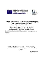
may reach near 10 to 15 %. Therefore, there is no mono-type of the shape and the magnitude
of the spectral water-leaving reflectance (Fig. 1). Inland and coastal waters may exhibit
bright, turbid waters due to phytoplankton and sediments or bottom reflectance of their
shallow areas, and in these cases simple thresholding techniques are no solution for the
extraction and delineation of water bodies.

Fig. 1. Surface reflectance spectra, R
S
(scale 0-1), of different inland waters (Rheinsberg Lake
District, Germany) representing different water colours (Reigber, in prep). GWUMM,
Grosser Wummsee, highly transparent, oligotrophic (nature reserve, densely forested);
ZOOTZ, Zootzensee, mesotroph (rural, forested); ZETHN, Zethner See, turbid, mesotroph-
eutrophic (rural); BRAMI, Braminsee, highly turbid, polytrophic (fish farming, rural)
3. Overview of existing methods for water body mapping
In the majority of algorithms for water body mapping a spectral band in the NIR spectral
region plays an important role due to the high absorption of water and resulting high

Remote Sensing of Planet Earth

6
contrast in NIR bands to many other surface types. However, Manavalan et al. (1993) found
that optimal cut-of gray values for individual spectral bands have to be carefully adjusted
and are varying between different images. Band ratios or spectral indices are often used to
mitigate spectral differences between images and also to enhance the contrast between
surface types. Consequently, indices like the NDWI (McFeeters, 1996) (Equation 1) and
MNDWI (Xu, 2006) (Equation 2) have been developed. Basically, the authors suggest a
default threshold value of zero for these indices, i.e. gray values greater than zero represent
water pixels. However, the comparative study of Ji et al. (2009) showed that an image and
landscape specific adjustment of threshold values can improve results. Therefore, these
methods are not fully suitable for automation. Further, NDWI shows high false positives in
build-up areas (Xu, 2006). Xu developed the MNDWI to enhance the separation between
water and built-up areas using Landsat ETM+ images. However, in high spatial resolution
images there is no single spectral profile for the class “built-up areas” (Roessner et al., 2011)
and many man-made materials have positive NDWI and/or MNDWI values (Fig. 2 and
Tab. 1). This is also true for shadow over non-vegetated areas. Fig. 3 shows that indices like
the NDWI are not suitable for water body mapping in urban areas using high spatial
resolution images since no threshold value can be found for which both, false positives and
false negatives are low.
MIR
NIR
green
Wavelength [nm]
2000
15001000500
1000
2000

3000
Reflectance [%
*
100]
Spectral profiles of selected surface types

Fig. 2. Reflectance spectra of man-made materials with positive NDWI and/or MNDWI
values. The gray bars indicate Landsat TM bands which are typically taken for calculating
the NDWI and MNDWI. The spectra were collected from the test site Potsdam
Surface type NDWI MNDWI
Copper 0.28 0.10
Plastic -0.13 0.01
Shadow 0.03 -0.10
PVC 0.03 0.20
Zinc 0.09 -0.17
Table 1. Corresponding index values of the spectra in Fig. 2
On the Use of Airborne Imaging Spectroscopy Data for the
Automatic Detection and Delineation of Surface Water Bodies

7



Fig. 3. True colour composite of an AISA image of Helgoland, Germany, with (b) histogram
of the NDWI, (c) Water mask by threshold 0 (red line in histogram) on the NDWI; (d) Water
mask by threshold 0.13 (green line in histogram) on the NDWI. In image c the water body
(bottom left side) is almost totally included in the water mask but many urban features are
so, too. In image d some parts of the water body are already lost but still some urban
features are present




green NIR
NDWI
green NIR




(1)
where green is a green band and NIR is a NIR band




green MIR
MNDWI
green MIR




(2)
where green is a green band and MIR is a middle infrared band
In addition to the spectral-based approaches object-oriented methods have been developed
for water body mapping (e.g. Xiao & Tien, 2010). However, since these methods use size and
shape features they have to be adjusted individually for each application and can not be
used for mapping ponds, rivers and coastal waters with the same configuration at the same
time.

Remote Sensing of Planet Earth

8
4. Material and methods
In this investigation a knowledge-based algorithm for the automated mapping of water
bodies was developed based on a spectral database from five airborne hyperspectral
datasets from the two German cities Berlin (two datasets) and Potsdam, and the German
island Helgoland (two datasets) (Tab. 2). Five independent datasets were used for validation
(Tab. 2). The selected scenes comprise urban, rural and coastal landscapes as well as
different sensors to prove the wide applicability of the developed approach. The AISA Eagle
sensor is an airborne VNIR pushbroom scanner (400 – 970 nm) with 12 bit radiometric
resolution and variable spatial and spectral binning options, the latter resulting in mean
spectral sampling intervals between 1.25 nm and 9.2 nm (Spectral Imaging Ltd., 2011) and

Test site Sensor Acquisition date, time (UTC) Pixel size (rounded)
Berlin (urban) HyMap
20.06.2005, 09:38 *
20.06.2005, 10:12 *
4 m
4 m
Potsdam (urban) HyMap 07.07.2004, 10:29 * 4 m
Helgoland (coastal) AISA Eagle
09.05.2008, 08:32 *
09.05.2008, 09:26 °
09.05.2008, 09:41 *
1 m
1 m
1 m
Rheinsberg (rural) HyMap 20.06.1999, 10:46 ° 10 m

Dresden (urban) HyMap 07.07.2004, 09:39 ° 4 m
Mönchsgut (coastal) HyMap 03.09.1998, 13:47 ° 6 m
Döberitzer Heide (rural) AISA Eagle 19.08.2009, 11:42 ° 2 m
* Datasets analyzed during algorithm development
° Independent datasets for validation
Table 2. Dataset-specific characteristics
Ammersee
Dresden
Döberitzer Heide
Berlin
Potsdam
Helgoland
Rheinsberg
AISA Eagle
HyMap
simulated EnMAP
Sensor types
urban
coastal
rural
Test site types
Mönchsgut

Fig. 4. Location of the test sites within Germany
On the Use of Airborne Imaging Spectroscopy Data for the
Automatic Detection and Delineation of Surface Water Bodies

9
488 to 60 spectral bands, respectively. The mean spectral sampling interval of the analyzed
datasets is 2.3 nm for “Döberitzer Heide” and 4.6 nm for “Helgoland”. The HyMap sensor is

an airborne VNIR-SWIR whiskbroom scanner with 16 bit radiometric resolution consisting
of four detector modules with mean spectral sampling intervals of 15 nm (VIS and NIR), 13
nm (SWIR1) and 17 nm (SWIR2) (Cocks et al., 1998). The 128 spectral bands cover the
spectral region from 440 nm to 2500 nm.
Water detection is a trivial task as long as there are no other dark surfaces present in the
image. Unfortunately, the most prominent spectral characteristic of water pixels – water
pixels are very dark – also applies to a couple of other surfaces such as dark rocks (e.g., lava,
basalt) or bituminous roofing materials and especially to pixels covered by shadow. To
account for this, we developed a two-step approach that firstly masks low albedo pixels as
potential water pixels (section 4.1) and secondly applies a process of elimination to
consecutively remove false positives (sections 4.2 and 4.3).
4.1 Masking potential water pixels
Masking of potential water pixels is done by thresholding a spectral mean image of all NIR
bands between 860 nm and 900 nm of a sensor. As pointed out before water absorbs most of
the incident energy in the NIR spectral region exhibiting a high brightness contrast to the
majority of other surfaces. However, since every scene is different a scene-specific threshold
has to be found. This is done automatically based on the histogram of the NIR spectral mean
image (Fig. 5). After finding the histogram peak of low albedo surfaces (first local
Histogram of NIR spectral mean image (Helgoland)
Number of pixels
Reflectance [%]
Subset for polynomial approximation (Helgoland)
Number of pixels
Reflectance [%]
Subset for polynomial approximation (Berlin)
Number of pixels
Reflectance [%]
Histogram of NIR spectral mean image (Berlin)
Number of pixels
Reflectance [%]

Fig. 5. Histograms (left: full, right: subset) of the NIR spectral mean images of two test sites
(top: Helgoland, bottom: Berlin)

Remote Sensing of Planet Earth

10
maximum) and a point near to the second local maximum (red dots in Fig. 5) the histogram
between these two points is approximated by a polynomial of degree 5 (magenta dashed
lines in Fig. 5). Then, the x value at the local minimum of the polynomial plus a safety
margin of 2 is taken as the maximum reflectance threshold to be applied on the NIR spectral
mean image. This results in a low albedo mask shown exemplarily for the test site Potsdam
in Fig. 6. From this mask the water pixels have to be identified and other low albedo
surfaces (mostly shadow) have to be removed.

Fig. 6. Low albedo mask (right-hand) for the test site Potsdam
4.2 Differentiation between macrophytes in water and vegetation under shadow on
land
Reflectance spectra of macrophytes (big emergent, submergent, or floating water plants) are
characterized by spectral features of vegetation, such as the chlorophyll absorption features
in the blue and red wavelength regions and the red edge in the NIR wavelength region. The
light absorbing properties of water result in reflectance spectra exhibiting a comparably low
albedo to those of shadowed vegetation on land (Fig. 7). Therefore, shadowed vegetation
cannot be removed from the low albedo mask by simply thresholding an NDVI image.

Fig. 7. Reflectance spectra of macrophytes in comparison with a reflectance spectrum of
shadowed vegetation on land. The blue bars mark the wavelength of the two ratios used for
distinguishing both surface types
On the Use of Airborne Imaging Spectroscopy Data for the
Automatic Detection and Delineation of Surface Water Bodies

11
However, a diagnostic spectral difference between both surfaces can be found in the NIR
spectral region where the increasing water absorption causes the reflectance spectra of
macrophytes to decrease between 710 – 740 nm as well as 815 – 880 nm. Therefore, pixels of
shadowed vegetation can be removed from the low albedo mask using the condition:
VI* > 1.0 AND (R
740
– R
710
/ 740 – 710 < -0.001 OR R
880
– R
815
/ 880 – 815 < -0.01) (3)
where
VI* = modified vegetation index = max(R
710
, R
720
) / R
680
R
740
= reflectance at wavelength 740 nm
Reflectance values must be scaled between 0 – 100
4.3 Removal of shadow pixels
Water and shadow reflectance spectra are on average both very dark. The reflectance level
of both decreases with wavelength due to a decreasing proportion of diffuse irradiation
(case of shadow) and due to the increasing light absorption (case of water). Additionally,

both show a high spectral variability due to different types of shadowed surfaces (case of
shadow) and due to varying water constituents and bottom reflection (case of water).
However, despite this variation all water reflectance spectra have one thing in common: the
pure water itself. Therefore, spectral features of pure water, especially absorption features,
can be seen in every reflectance spectrum of water. However, the presence of these spectral
features depends on the spectral superimposition of the water constituents and bottom
coverage. Section 4.3.1 describes how these aspects can be considered in the development of
a knowledge-based classifier for spectrally distinguishing water and shadow. Section 4.3.2
then continues with a spatial analysis.
4.3.1 Spectral analysis for water-shadow-separation based on spectral slopes
Fig. 8 shows the absorption spectrum of pure water (logarithmic scale) in comparison with
selected surface reflectance spectra of different water bodies of the analyzed datasets. It can
be seen that the increasing absorption within specific wavelength intervals (1
st
, 2
nd
, 4
th
and
5
th
light red bar) results in decreasing reflectance for most of the reflectance spectra. The 3
rd

light red bar represents a short wavelength interval of stagnating absorption where some
water reflectance spectra temporarily rise due to increasing reflectance of water constituents
or water bottom before decreasing again. However, these effects are not present within all
wavelength intervals of all water reflectance spectra because they can be superimposed by
the reflectance of the water constituents and water bottom. In order to find the slope
combinations that occur for typical water bodies we analyzed 112.041 surface reflectance

spectra from five datasets (two from Helgoland, two from Berlin, one from Potsdam). The
selected datasets contain several types of water bodies (rivers, lakes, ponds, North Sea;
transparent to productive and turbid waters). A first-degree polynomial was fitted to the
spectra within each of the five wavelength intervals using the least squares method. If the
algebraic sign of the slope within a wavelength interval met the expectation it was coded to
1 otherwise to 0. This resulted in a five-digit binary vector for each analyzed water
reflectance spectrum representing the co-occurrence of slopes within the respective
diagnostic wavelength intervals that met the expectation. The 25 possible binary vectors

Remote Sensing of Planet Earth

12
were numbered from 0 to 31 whereas the 0 vector (none of the 5 slopes met the expectation)
was excluded from further analysis. The numbered combinations are shown in Fig. 9 in
comparison with the numbered combinations of 33.721 analyzed shadow spectra. It can be
seen that many combinations are occupied either by water or by shadow spectra and thus
provide a clear separation between water and shadow. These combinations are
implemented in the developed approach so that applied to an image many pixels of the low
albedo mask can either be identified as water or rejected as shadow. The other combinations
marked by the orange arrows are ambiguous. Pixels that fall into these combinations need a
consecutive spatial processing described in Section 4.3.2.
Water absorption vs water reflectance
Wavelength [nm]
450 500 550 600 650 700 750 800 850 900


Fig. 8. Absorption of pure water (thick blue line, logarithmic scale, source: WASI (Gege,
2005)) in comparison to water surface reflectance spectra from different water bodies of the
analyzed datasets. The increasing absorption within specific wavelength intervals (light red
bars) results in decreasing reflectance for most of the reflectance spectra but is partly

superimposed by the reflectance of the water constituents and water bottom
On the Use of Airborne Imaging Spectroscopy Data for the
Automatic Detection and Delineation of Surface Water Bodies

13
Relative frequency of the slope combinations for water and shadow areas
0
5
10
15
20
25
30
35
1 3 5 7 9 11 13 15 17 19 21 23 25 27 29 31
Combination number
Relative frequency
Water
Shadow

Fig. 9. Numbered slope combinations for water and shadow reflectance spectra. Due to the
different amount of analyzed pixels of water and shadow (112.041 and 33.721) the relative
frequency per land cover class is given. Combinations that are occupied by only one bar (or
one very big and one very small bar) provide a clear separation between water and shadow.
The combinations marked by the orange arrows are spectrally ambiguous
4.3.2 Spatial analysis for water-shadow-separation
Pixels of the low albedo mask that have not been identified as water or shadow based on the
unambiguous spectral slope combinations are subjected to a consecutive spatial analysis. In
this processing the idea is to decide according to the dominating spectral decision (see
previous section) made within the neighbourhood of the ambiguous pixels (Fig. 10). The

spectral decisions in the neighbourhood are counted using a 3x3 filter kernel resulting in a
water score and a no-water score for each ambiguous pixel. If one of the two scores is more
than three times higher than the other the ambiguous pixel is either identified as water or as
no-water and is written into the respective image of confirmed water or no-water areas. If this
is not the case the filter kernel iteratively grows up to a size of 33x33. Thereby, the identified
water and no-water pixels are written into the respective image of identified water or no-water
areas after each iteration so that they can be counted by the filter of the following iterations.
When the filter kernel has reached a size of 33x33 and there are still ambiguous pixels left the
decision threshold is reduced to two times higher than the other score and the filter kernel is
reset to a size of 3x3. When the filter kernel reached a size of 33x33 for the second time it is
again reset to a size of 3x3 and the decision is then simply related to the higher score. At this
stage the filter starts growing again without a limit and until a decision was made for every
ambiguous pixel. The graduation of the decision threshold has the advantage that pixels with
an unambiguous neighbourhood are confirmed first and then accounted for in the following
iterations. Finally, after all pixels have been identified either by spectral or spatial processing,
the spectrally or spatially identified water pixels are combined into the final water mask. A last

Remote Sensing of Planet Earth

14
Spectrally
identified water
No spectral
decision
Spectrally
rejected no-water
Neighborhood
analysis
Water score
Spatially

identified water
No-water score
Spatially
rejected no-water
100
10
1
0
Water mask
+ spectrally
identified water

Fig. 10. Spatial processing illustrated by an exemplary subset of the Potsdam test site
aesthetic correction is done by filling up one pixel wholes within water areas which are
considered as errors induced by noise. The filling of wholes can optionally be extended onto
larger wholes (up to a certain size) which are likely to be boats (see Fig. 11).
On the Use of Airborne Imaging Spectroscopy Data for the
Automatic Detection and Delineation of Surface Water Bodies

15




Fig. 11. (continued)