- Trang chủ >>
- Khoa Học Tự Nhiên >>
- Vật lý
remote sensing of environment
Bạn đang xem bản rút gọn của tài liệu. Xem và tải ngay bản đầy đủ của tài liệu tại đây (2.28 MB, 32 trang )
Introduction to Remote Sensing
page 1
Remote Sensing of
Environment (RSE)
with
TNTmips
®
TNTview
®
Introduction to
I
N
T
R
O
T
O
R
S
E
Introduction to Remote Sensing
page 2
Before Getting Started
You can print or read this booklet in color from MicroImages’ Web site. The
Web site is also your source for the newest tutorial booklets on other topics.
You can download an installation guide, sample data, and the latest version
of TNTmips.
Imagery acquired by airborne or satellite sensors provides an important source of
information for mapping and monitoring the natural and manmade features on the
land surface. Interpretation and analysis of remotely sensed imagery requires an
understanding of the processes that determine the relationships between the prop-
erty the sensor actually measures and the surface properties we are interested in
identifying and studying. Knowledge of these relationships is a prerequisite for
appropriate processing and interpretation. This booklet presents a brief overview
of the major fundamental concepts related to remote sensing of environmental
features on the land surface.
Sample Data The illustrations in this booklet show many examples of remote
sensing imagery. You can find many additional examples of imagery in the sample
data that is distributed with the TNT products. If you do not have access to a TNT
products CD, you can download the data from MicroImages’ Web site. In particu-
lar, the CB_DATA, SF_DATA, BEREA, and COMBRAST data collections include sample
files with remote sensing imagery that you can view and study.
More Documentation This booklet is intended only as an introduction to basic
concepts governing the acquisition, processing, and interpretation of remote sensing
imagery. You can view all types of imagery in TNTmips using the standard Dis-
play process, which is introduced in the tutorial booklet entitled Displaying
Geospatial Data. Many other processes in TNTmips can be used to process,
enhance, or analyze imagery. Some of the most important ones are mentioned on
the appropriate pages in this booklet, along with a reference to an accompanying
tutorial booklet.
TNTmips
®
Pro and TNTmips Free
TNTmips (the Map and Image Processing
System) comes in three versions: the professional version of TNTmips (TNTmips
Pro), the low-cost TNTmips Basic version, and the TNTmips Free version. All
versions run exactly the same code from the TNT products DVD and have nearly
the same features. If you did not purchase the professional version (which re-
quires a software license key) or TNTmips Basic, then TNTmips operates in
TNTmips Free mode.
Randall B. Smith, Ph.D., 4 January 2012
©MicroImages, Inc., 2001–2012
Introduction to Remote Sensing
page 3
Introduction to Remote Sensing
Remote sensing is the sci-
ence of obtaining and
interpreting information
from a distance, using sen-
sors that are not in physical
contact with the object be-
ing observed. Though you
may not realize it, you are
familiar with many examples. Biological evolution
has exploited many natural phenomena and forms
of energy to enable animals (including people) to
sense their environment. Your eyes detect electro-
magnetic energy in the form of visible light. Your
ears detect acoustic (sound) energy, while your nose
contains sensitive chemical receptors that respond
to minute amounts of airborne chemicals given off
by the materials in our surroundings. Some research
suggests that migrating birds can sense variations in
Earth’s magnetic field, which helps explain their re-
markable navigational ability.
The science of remote sensing in its broadest sense
includes aerial, satellite, and spacecraft observations
of the surfaces and atmospheres of the planets in
our solar system, though the Earth is obviously the
most frequent target of study. The term is customar-
ily restricted to methods that detect and measure
electromagnetic energy, including visible light, that
has interacted with surface materials and the atmo-
sphere. Remote sensing of the Earth has many
purposes, including making and updating planimet-
ric maps, weather forecasting, and gathering military
intelligence. Our focus in this booklet will be on
remote sensing of the environment and resources of
Earth’s surface. We will explore the physical con-
cepts that underlie the acquisition and interpretation
of remotely sensed images, the important character-
istics of images from different types of sensors, and
some common methods of processing images to en-
hance their information content.
Fundamental concepts of
electromagnetic radiation
and its interactions with
surface materials and the
atmosphere are introduced
on pages 4-9. Image
acquisition and various
concepts of image
resolution are discussed on
pages 10-16. Pages 17-23
focus on images acquired in
the spectral range from
visible to middle infrared
radiation, including visual
image interpretation and
common processes used to
correct or enhance the
information content of
multispectral images.
Pages 23-24 discuss
images acquired on multiple
dates and their spatial
registration and
normalization. You can
learn some basic concepts
of thermal infrared imagery
on pages 26-27, and radar
imagery on pages 28-29.
Page 30 presents an
example of combine
images from different
sensors. Sources of
additional information on
remote sensing are listed
on page 31.
Artist’s depiction of the
Landsat 7 satellite in
orbit, courtesy of
NASA. Launched in
late 1999, this satellite
acquires multispectral
images using reflected
visible and infrared ra-
diation.
Introduction to Remote Sensing
page 4
The Electromagnetic Spectrum
The field of remote sensing began with aerial pho-
tography, using visible light from the sun as the
energy source. But visible light makes up only a
small part of the electromagnetic spectrum, a con-
tinuum that ranges from high energy, short
wavelength gamma rays, to lower energy, long wave-
length radio waves. Illustrated below is the portion
of the electromagnetic spectrum that is useful in re-
mote sensing of the Earth’s surface.
The Earth is naturally illuminated by electromagnetic
radiation from the Sun. The peak solar energy is in
the wavelength range of visible light (between 0.4
and 0.7 µm). It’s no wonder that the visual systems
of most animals are sensitive to these wavelengths!
Although visible light includes the entire range of
colors seen in a rainbow, a cruder subdivision into
blue, green, and red wavelength regions is sufficient
in many remote sensing studies. Other substantial
fractions of incoming solar energy are in the form of
invisible ultraviolet and infrared radiation. Only tiny
amounts of solar radiation extend into the microwave
region of the spectrum. Imaging radar systems used
in remote sensing generate and broadcast micro-
waves, then measure the portion of the signal that
has returned to the sensor from the Earth’s surface.
Electromagnetic radiation
behaves in part as wavelike
energy fluctuations traveling
at the speed of light. The
wave is actually composite,
involving electric and mag-
netic fields fluctuating at right
angles to each other and to
the direction of travel.
A fundamental descriptive
feature of a waveform is its
wavelength, or distance be-
tween succeeding peaks or
troughs. In remote sensing,
wavelength is most often
measured in micrometers,
each of which equals one
millionth of a meter. The
variation in wavelength of
electromagnetic radiation is
so vast that it is usually
shown on a logarithmic scale.
UNITS
1 micrometer (µm) = 1 x 10
-6
meters
1 millimeter (mm) = 1 x 10
-3
meters
1 centimeter (cm) = 1 x 10
-2
meters
Wavelength
Wavelength
(logarithmic scale)
Incoming from Sun
Emitted by Earth
0.4 0.5 0.6 0.7
Blue Green Red
MICROWAVE
(RADAR)
INFRARED
1 m10 cm1 cm
100 µm10 µm1 µm
1 mm
0.1 µm
VISIBLE
ULTRAVIOLET
Energy
Introduction to Remote Sensing
page 5
Interaction Processes
Remote sensors measure electromagnetic (EM) ra-
diation that has interacted with the Earth’s surface.
Interactions with matter can change the direction,
intensity, wavelength content, and polarization of EM
radiation. The nature of these changes is dependent
on the chemical make-up and physical structure of
the material exposed to the EM radiation. Changes
in EM radiation resulting from its interactions with
the Earth’s surface therefore provide major clues to
the characteristics of the surface materials.
The fundamental interactions between EM radiation
and matter are diagrammed to the right. Electro-
magnetic radiation that is transmitted passes through
a material (or through the boundary between two
materials) with little change in intensity. Materials
can also absorb EM radiation. Usually absorption
is wavelength-specific: that is, more energy is ab-
sorbed at some wavelengths than at others. EM
radiation that is absorbed is transformed into heat
energy, which raises the material’s temperature.
Some of that heat energy may then be emitted as
EM radiation at a wavelength dependent on the
material’s temperature. The lower the temperature,
the longer the wavelength of the emitted radiation.
As a result of solar heating, the Earth’s surface emits
energy in the form of longer-wavelength infrared
radiation (see illustration on the preceding page). For
this reason the portion of the infrared spectrum with
wavelengths greater than 3 µm is commonly called
the thermal infrared region.
Electromagnetic radiation encountering a boundary
such as the Earth’s surface can also be reflected. If
the surface is smooth at a scale comparable to the
wavelength of the incident energy, specular reflec-
tion occurs: most of the energy is reflected in a single
direction, at an angle equal to the angle of incidence.
Rougher surfaces cause scattering, or diffuse reflec-
tion in all directions.
Matter - EM Energy
Interaction Processes
The horizontal line
represents a boundary
between two materials.
Specular Reflection
Scattering
(Diffuse Reflection)
Absorption
Emission
Transmission
Introduction to Remote Sensing
page 6
Interaction Processes in Remote Sensing
Typical EMR interactions in the atmosphere and at the Earth’s surface.
To understand how different interaction processes impact the acquisition of aerial
and satellite images, let’s analyze the reflected solar radiation that is measured at
a satellite sensor. As sunlight initially enters the atmosphere, it encounters gas
molecules, suspended dust particles, and aerosols. These materials tend to scatter
a portion of the incoming radiation in all directions, with shorter wavelengths
experiencing the strongest effect. (The preferential scattering of blue light in
comparison to green and red light accounts for the blue color of the daytime sky.
Clouds appear opaque because of intense scattering of visible light by tiny water
droplets.) Although most of the remaining light is transmitted to the surface,
some atmospheric gases are very effective at absorbing particular wavelengths.
(The absorption of dangerous ultraviolet radiation by ozone is a well-known ex-
ample). As a result of these effects, the illumination reaching the surface is a
combination of highly filtered solar radiation transmitted directly to the ground
and more diffuse light scattered from all parts of the sky, which helps illuminate
shadowed areas.
As this modified solar radiation reaches the ground, it may encounter soil, rock
surfaces, vegetation, or other materials that absorb a portion of the radiation. The
amount of energy absorbed varies in wavelength for each material in a character-
istic way, creating a sort of spectral signature. (The selective absorption of different
wavelengths of visible light determines what we perceive as a material’s color).
Most of the radiation not absorbed is diffusely reflected (scattered) back up into
the atmosphere, some of it in the direction of the satellite. This upwelling radia-
tion undergoes a further round of scattering and absorption as it passes through
the atmosphere before finally being detected and measured by the sensor. If the
sensor is capable of detecting thermal infrared radiation, it will also pick up radia-
tion emitted by surface objects as a result of solar heating.
EMR
Source
Sensor
Absorption
Absorption
Absorption
Scattering
Scattering
Scattering
Scattering
Emission
Transmission
Introduction to Remote Sensing
page 7
Atmospheric Effects
Scattering and absorption of EM radiation by the at-
mosphere have significant effects that impact sensor
design as well as the processing and interpretation
of images. When the concentration of scattering
agents is high, scattering produces the visual effect
we call haze. Haze increases the overall brightness
of a scene and reduces the contrast between different
ground materials. A hazy atmosphere scatters some
light upward, so a portion of the radiation recorded
by a remote sensor, called path radiance, is the re-
sult of this scattering process. Since the amount of
scattering varies with wavelength, so does the con-
tribution of path radiance to remotely sensed images.
As shown by the figure to the right, the path radi-
ance effect is greatest for the shortest wavelengths,
falling off rapidly with increasing wavelength. When
images are captured over several wavelength ranges,
the differential path radiance effect complicates com-
parison of brightness values at the different
wavelengths. Simple methods for correcting for path
radiance are discussed later in this booklet.
The atmospheric components that are effective ab-
sorbers of solar radiation are water vapor, carbon
dioxide, and ozone. Each of these gases tends to
absorb energy in specific wavelength ranges. Some
wavelengths are almost completely absorbed. Con-
sequently, most broad-band remote sensors have been
designed to detect radiation in the “atmospheric win-
dows”, those wavelength ranges for which absorption
is minimal, and, conversely, transmission is high.
Relative Scattering
0.4 0.6 0.8 1.0
Wavelength,
µµ
µµ
µm
Range of scattering for
typical atmospheric
conditions (colored area)
versus wavelength.
Scattering increases with
increasing humidity and
particulate load but
decreases with increasing
wavelength. In most cases
the path radiance produced
by scattering is negligible at
wavelengths longer than
the near infrared.
100
1 m
0.3 µm1 µm 10 µm 100 µm
1 mm
Transmission (%)
0
Visible
Ultraviolet
Thermal
Infrared
Near IR
Middle
IR
Microwave
Variation in atmospheric
transmission with
wavelength of EM radiation,
due to wavelength-selective
absorption by atmospheric
gases. Only wavelength
ranges with moderate to
high transmission values
are suitable for use in
remote sensing.
Introduction to Remote Sensing
page 8
All remote sensing systems designed to monitor the Earth’s surface rely on energy
that is either diffusely reflected by or emitted from surface features. Current re-
mote sensing systems fall into three categories on the basis of the source of the
electromagnetic radiation and the relevant interactions of that energy with the
surface.
Reflected solar radiation sensors These sensor systems detect solar radiation
that has been diffusely reflected (scattered) upward from surface features. The
wavelength ranges that provide useful information include the ultraviolet, visible,
near infrared and middle infrared ranges. Reflected solar sensing systems dis-
criminate materials that have differing patterns of wavelength-specific absorption,
which relate to the chemical make-up and physical struc-
ture of the material. Because they depend on sunlight as
a source, these systems can only provide useful images
during daylight hours, and changing atmospheric condi-
tions and changes in illumination with time of day and
season can pose interpretive problems. Reflected solar
remote sensing systems are the most common type used
to monitor Earth resources, and are the primary focus of
this booklet.
Thermal infrared sensors Sensors that can detect the
thermal infrared radiation emitted by surface features
can reveal information about the thermal properties of
these materials. Like reflected solar sensors, these are
passive systems that rely on solar radiation as the ulti-
mate energy source. Because the temperature of surface
features changes during the day, thermal infrared sens-
ing systems are sensitive to time of day at which the
images are acquired.
Imaging radar sensors Rather than relying on a natural source, these “active”
systems “illuminate” the surface with broadcast micro-
wave radiation, then measure the energy that is diffusely
reflected back to the sensor. The returning energy pro-
vides information about the surface roughness and water
content of surface materials and the shape of the land
surface. Long-wavelength microwaves suffer little scat-
tering in the atmosphere, even penetrating thick cloud
cover. Imaging radar is therefore particularly useful in
cloud-prone tropical regions.
EMR Sources, Interactions, and Sensors
Reflected red image
Thermal Infrared image
Radar image
Introduction to Remote Sensing
page 9
Spectral Signatures
The spectral signatures produced by wavelength-dependent absorption provide
the key to discriminating different materials in images of reflected solar energy.
The property used to quantify these spectral signatures is called spectral reflec-
tance: the ratio of reflected energy to incident energy as a function of wavelength.
The spectral reflectance of different materials can be measured in the laboratory
or in the field, providing reference data that can be used to interpret images. As an
example, the illustration below shows contrasting spectral reflectance curves for
three very common natural materials: dry soil, green vegetation, and water.
The reflectance of dry soil rises uniformly through the visible and near infrared
wavelength ranges, peaking in the middle infrared range. It shows only minor
dips in the middle infrared range due to absorption by clay minerals. Green veg-
etation has a very different spectrum. Reflectance is relatively low in the visible
range, but is higher for green light than for red or blue, producing the green color
we see. The reflectance pattern of green vegetation in the visible wavelengths is
due to selective absorption by chlorophyll, the primary photosynthetic pigment in
green plants. The most noticeable feature of the vegetation spectrum is the dra-
matic rise in reflectance across the visible-near infrared boundary, and the high
near infrared reflectance. Infrared radiation penetrates plant leaves, and is in-
tensely scattered by the leaves’ complex internal structure, resulting in high
reflectance. The dips in the middle infrared portion of the plant spectrum are due
to absorption by water. Deep clear water bodies effectively absorb all wavelengths
longer than the visible range, which results in very low reflectivity for infrared
radiation.
Reflectance
0
0.2
0.4
0.6
0.4 0.6 0.8 1.0 1.2 1.4 1.6 1.8 2.0 2.2 2.4 2.6
Wavelength (
µµ
µµ
µm)
Clear Water Body
Green Vegetation
Dry Bare Soil
Near Infrared
Middle Infrared
Red
Grn
Blue
Reflected Infrared
Introduction to Remote Sensing
page 10
Image Acquisition
52
71
74
102
113 144 1196570
6489 125 90
6687 87 80
89111 77 95
111115 67 74
We have seen that the radiant energy that is measured by an aerial or satellite
sensor is influenced by the radiation source, interaction of the energy with surface
materials, and the passage of the energy through the atmosphere. In addition, the
illumination geometry (source position, surface slope, slope direction, and shad-
owing) can also affect the brightness of the upwelling energy. Together these
effects produce a composite “signal” that varies spatially and with the time of day
or season. In order to produce an image which we can interpret, the remote sens-
ing system must first detect and measure this energy.
The electromagnetic energy returned from the Earth’s surface can be detected by
a light-sensitive film, as in aerial photography, or by an array of electronic sen-
sors. Light striking photographic film causes a chemical
reaction, with the rate of the reaction varying with the
amount of energy received by each point on the film.
Developing the film converts the pattern of energy varia-
tions into a pattern of lighter and darker areas that can
be interpreted visually.
Electronic sensors generate an electrical signal with
a strength proportional to the amount of energy
received. The signal from each detector in an
array can be recorded and transmitted elec-
tronically in digital form (as a series of
numbers). Today’s digital still and video cam-
eras are examples of imaging systems that use
electronic sensors. All modern satellite imag-
ing systems also use some form of electronic
detectors.
An image from an electronic sensor array (or
a digitally scanned photograph) consists of a
two-dimensional rectangular grid of numeri-
cal values that represent differing brightness
levels. Each value represents the average
brightness for a portion of the surface, represented by
the square unit areas in the image. In computer terms
the grid is commonly known as a raster, and the square
units are cells or pixels. When displayed on your com-
puter, the brightness values in the image raster are
translated into display brightness on the screen.
Introduction to Remote Sensing
page 11
Spatial Resolution
The spatial, spectral, and temporal components of
an image or set of images all provide information
that we can use to form interpretations about sur-
face materals and conditions. For each of these
properties we can define the resolution of the im-
ages produced by the sensor system. These image
resolution factors place limits on what information
we can derive from remotely sensed images.
Spatial resolution is a measure of the spatial detail
in an image, which is a function of the design of the
sensor and its operating altitude above the surface.
Each of the detectors in a remote sensor measures
energy received from a finite patch of the ground
surface. The smaller these individual patches are,
the more detailed will be the spatial information that
we can interpret from the image. For digital images,
spatial resolution is most commonly expressed as the
ground dimensions of an image cell.
Shape is one visual factor that we can use to recog-
nize and identify objects in an image. Shape is usually
discernible only if the object dimensions are several
times larger than the cell dimensions.
On the other hand, objects smaller
than the image cell size may be de-
tectable in an image. If such an
object is sufficiently brighter or
darker than its surroundings, it will
dominate the averaged brightness of
the image cell it falls within, and that
cell will contrast in brightness with
the adjacent cells. We may not be able to identify
what the object is, but we can see that something is
present that is different from its surroundings, espe-
cially if the “background” area is relatively uniform.
Spatial context may also allow us to recognize linear
features that are narrower than the cell dimensions,
such as roads or bridges over water. Evidently there
is no clear dimensional boundary between detectabil-
ity and recognizability in digital images.
The image above is a portion
of a Landsat Thematic Map-
per scene showing part of
San Francisco, California.
The image has a cell size of
28.5 meters. Only larger
buildings and roads are
clearly recognizable. The
boxed area is shown below
left in an IKONOS image with
a cell size of 4 meters. Trees,
smaller buildings, and nar-
rower streets are recogniz-
able in the Ikonos image.
The bottom image shows the
boxed area of the
Thematic Mapper
scene enlarged
to the same scale
as the IKONOS
image, revealing
the larger cells in
the Landsat im-
age.
Introduction to Remote Sensing
page 12
The spectral resolution of a remote sensing system can be described as its ability
to distinguish different parts of the range of measured wavelengths. In essence,
this amounts to the number of wavelength intervals (“bands”) that are measured,
and how narrow each interval is. An “image” produced by a sensor system can
consist of one very broad wavelength band, a few broad bands, or many narrow
wavelength bands. The names usually used for these three image categories are
panchromatic, multispectral, and hyperspectral, respectively.
Aerial photographs taken using black and white film record an average response
over the entire visible wavelength range (blue, green, and red). Because this film
is sensitive to all visible colors, it is called panchromatic film. A panchromatic
image reveals spatial variations in the gross visual properties of surface materials,
but does not allow spectral discrimination. Some satellite remote sensing sys-
tems record a single very broad band to provide a synoptic overview of the scene,
commonly at a higher spatial resolution than other sensors on board. Despite
varying wavelength ranges, such bands are also commonly referred to as panchro-
matic bands. For example, the sensors on the first three SPOT satellites included
a panchromatic band with a spectral range of 0.51 to 0.73 micrometers (green and
red wavelength ranges). This band has a spatial resolution of 10 meters, in con-
trast to the 20-meter resolution of the multispectral sensor bands. The panchromatic
band of the Enhanced The-
matic Mapper Plus sensor
aboard NASA’s Landsat 7 sat-
ellite covers a wider spectral
range of 0.52 to 0.90 microme-
ters (green, red, and near
infrared), with a spatial reso-
lution of 15 meters (versus
30-meters for the sensor’s
multispectral bands).
Spectral Resolution
SPOT panchromatic image of
part of Seattle, Washington.
This image band spans the
green and red wavelength
ranges. Water and vegetation
appear dark, while the brightest
objects are building roofs and a
large circular tank.
Introduction to Remote Sensing
page 13
In order to provide increased spectral discrimination, remote sensing systems de-
signed to monitor the surface environment employ a multispectral design: parallel
sensor arrays detecting radiation in a small number of broad wavelength bands.
Most satellite systems use from three to six spectral bands in the visible to middle
infrared wavelength region. Some systems also employ one or more thermal in-
frared bands. Bands in the infrared range are limited in width to avoid atmospheric
water vapor absorption effects that significantly degrade the signal in certain wave-
length intervals (see the previous page Atmospheric Effects). These broad-band
multispectral systems allow discrimination of different types of vegetation, rocks
and soils, clear and turbid water, and some man-made materials.
A three-band sensor with green, red, and near infrared bands is effective at dis-
criminating vegetated and nonvegetated areas. The HRV sensor aboard the French
SPOT (Système Probatoire d’Observation de la Terre) 1, 2, and 3 satellites (20
meter spatial resolution) has this design. Color-infrared film used in some aerial
photography provides similar spectral coverage, with the red emulsion recording
near infrared, the green emulsion recording red light, and the blue emulsion re-
cording green light. The IKONOS satellite from Space Imaging (4-meter
resolution) and the LISS II sensor on the Indian Research Satellites IRS-1A and
1B (36-meter resolution) add a blue band to provide complete coverage of the
visible light range, and allow natural-color band
composite images to be created. The Landsat
Thematic Mapper (Landsat 4 and 5) and En-
hanced Thematic Mapper Plus (Landsat
7) sensors add two bands in the middle
infrared (MIR). Landsat TM band 5
(1.55 to 1.75 µm) and band 7 (2.08 to
2.35 µm) are sensitive to variations in
the moisture content of vegetation and
soils. Band 7 also covers a range that
includes spectral absorption features
found in several important types of minerals. An additional TM band (band 6)
records part of the thermal infrared wavelength range (10.4 to 12.5 µm). (Bands
6 and 7 are not in wavelength order because band 7 was added late in the sensor
design process.) Current multispectral satellite sensor systems with spatial reso-
lution better than 200 meters are compared on the following pages.
To provide even greater spectral resolution, so-called hyperspectral sensors make
measurements in dozens to hundreds of adjacent, narrow wavelength bands (as
little as 0.1 µm in width). For more information on these systems, see the booklet
Introduction to Hyperspectral Imaging.
Multispectral Images
Introduction to Remote Sensing
page 14
Multispectral Satellite Sensors
Platform /
Sensor /
Launch Yr.
Image
Cell
Size
Image Size
(Cross x
Along-Track)
Spec.
Bands
Visible
Bands
(
µµ
µµ
µm)
Near IR
Bands
(
µµ
µµ
µm)
Ikonos-2
VNIR
1999
Terra
(EOS-AM-1)
ASTER
1999
SPOT 4
HRVIR (XS)
1999
Landsat 7
ETM+
1999
Landsat 4, 5
TM
1982
4 m 11 x 11 km 4 B 0.45-0.52
G 0.52-0.60
R 0.63-0.69
0.76-0.90
15 m
(Vis, NIR)
30 m
(MIR)
90 m
(TIR)
60 x 60 km 14 G 0.52-0.60
R 0.63-0.69
0.76-0.86
20 m 60 x 60 km 4 G 0.50-0.59
R 0.61-0.68
0.79-0.89
30 m 185 x 170 km 7 B 0.45-0.515
G 0.525-0.605
R 0.63-0.69
0.75-0.90
30 m 185 x 170 km 7 B 0.45-0.52
G 0.52-0.60
R 0.63-0.69
0.76-0.90
Ikonos-2: Space Imaging, Inc., USA ResourceSAT-2: Indian Space Research Org.
Terra, Landsat: NASA, USA QuickBird, WorldView: DigitalGlobe, Inc., USA
SPOT: Centre National d’Etudes Spatiales (CNES), France
SPOT 5
HRG
2002
10 m
(Vis, NIR)
20 m (MIR)
60 x 60 km 4 G 0.50-0.59
R 0.61-0.68
0.79-0.89
QuickBird
2001
2.4 or 2.8
m
16.5 x 16.5 km 4 B 0.45-0.52
G 0.52-0.60
R 0.63-0.69
0.76-0.90
RapidEye
2008
6.5 m 77 km 5 B 0.44-0.51
G 0.52-0.59
R 0.63-0.685
0.69-0.73
0.76-0.85
GeoEye-1
2008
1.65 m 15 x 15 km 4 B 0.45-0.51
G 0.51-0.58
R 0.655-0.69
0.78-0.92
ResourceSAT-2
2011
5.8 m
(LISS-4)
70 km 3 G 0.52-0.59
R 0.62-0.68
0.77-0.86
23.5 m
(LISS-3)
3 G 0.52-0.59
R 0.62-0.68
0.77-0.86
WorldView-2
2009
1.8 m 16.4 km 8 0.40-0.45
B 0.45-0.51
G 0.51-0.58
Y 0.585-0.625
R 0.655-0.69
0.705-0.745
0.860-1.04
Introduction to Remote Sensing
page 15
Satellite Sensors Table (Continued)
Mid. IR
Bands
(
µµ
µµ
µm)
Thermal
IR Bands
(
µµ
µµ
µm)
Panchrom.
Band
Range (
µµ
µµ
µm)
None None
Pan
Cell
Size
1.60-1.70
2.145-2.185
2.185-2.225
2.235-2.285
2.295-2.365
2.36-2.43
8.125-8.475
8.475-8.825
8.925-9.275
10.25-10.95
10.95-11.65
0.45-0.90
B, G, R, NIR
Nominal
Revisit
Interval*
1 m 11 days
(2.9 days
†
)
None X 16 days
1.58-1.75 None 0.61-0.68
R
10 m 26 days
(5 days
†
)
1.55-1.75
2.09-2.35
10.40-12.50 0.52-0.90
G, R, NIR
15 m 16 days
1.55-1.75
2.08-2.35
10.40-12.50 None X 16 days
* Single satellite, nadir
view at equator
†
With off-nadir pointing
You can import imagery from any of these sensors into the
TNTmips Project File format using the Import / Export process.
Each image band is stored as a raster object.
Platform /
Sensor /
Launch Yr.
Ikonos-2
VNIR
1999
Terra
(EOS-AM-1)
ASTER
1999
SPOT 4
HRVIR (XS)
1999
Landsat 7
ETM+
1999
Landsat 4, 5
TM
1982
SPOT 5
HRG
2002
1.58-1.75 None 0.51-0.73
G, R
5 m 26 days
(3 days
†
)
QuickBird
2001
None None 0.45-0.90
B, G, R, NIR
0.6 or
0.7 m
(3.5 days
†
)
RapidEye
2008
None None None X
5.5 days
(1 day
†
)
GeoEye-1
2008
None None 0.45-0.80
B, G, R, NIR
0.41 m
5.5 days
(1 day
†
)
ResourceSAT-2
2011
None None None X
24 days
(5 days
†
)
1.55-1.70 None None X
WorldView-2
2009
None None 0.45-0.80
B, G, R, NIR
0.41 m
3.7 days
(1.1 day
†
)
Introduction to Remote Sensing
page 16
In order to digitally record the energy received by an individual detector in a
sensor, the continuous range of incoming energy must be quantized, or subdi-
vided into a number of discrete levels that are recorded as integer values. Many
current satellite systems quantize data into 256 levels (8 bits of data in a binary
encoding system). The thermal infrared bands of the ASTER sensor are quan-
tized into 4096 levels (12 bits). The more levels that can be recorded, the greater
is the radiometric resolution of the sensor system.
High radiometric resolution is advantageous when you use a computer to process
and analyze the numerical values in the bands of a multispectral image. (Several
of the most common analysis procedures, band ratio analysis and spectral classi-
fication, will be described subsequently.) Visual analysis of multispectral images
also benefits from high radiometric resolution because
a selection of wavelength bands can be combined to
form a color display or print. One band is assigned to
each of the three color channels used by the computer
monitor: red, green, and blue. Using the additive color
model, differing levels of these three primary colors
combine to form millions of subtly different colors.
For each cell in the multispectral image, the bright-
ness values in the selected bands determine the red,
green, and blue values used to create the displayed
color. Using 256 levels for each color channel, a
computer display can create over 16 million col-
ors. Experiments indicate that the human visual
system can distinguish close to seven million col-
ors, and it is also highly attuned to spatial
relationships. So despite the power of computer
analysis, visual analysis of color displays of multi-
spectral imagery can still be an effective tool in
their interpretation.
Individual band images in the visible to middle in-
frared range from the Landsat Thematic Mapper are illustrated for two sample
areas on the next page. The left image is a mountainous terrane with forest (lower
left), bare granitic rock, small clear lakes, and snow patches. The right image is
an agricultural area with both bare and vegetated fields, with a town in the upper
left and yellowed grass in the upper right. The captions for each image pair dis-
cuss some of the diagnostic uses of each band. Many color combinations are also
possible with these six image bands. Three of the most widely-used color combi-
nations are illustrated on a later page.
Radiometric Resolution
RG
B
Y
C
M
Introduction to Remote Sensing
page 17
Visible to Middle Infrared Image Bands
Blue (TM 1): Provides maximum penetration
of shallow water bodies, though the mountain
lakes in the left image are deep and thus appear
dark, as does the forested area. In the right
image, the town and yellowed grassy areas are
brighter than the bare and cultivated agricultural
fields. The brightness of the bare fields varies
widely with moisture content.
Green (TM 2): Includes the peak visible light
reflectance of green vegetation, thus helps
assess plant vigor and differentiate green and
yellowed vegetation. But note that forest is still
darker than bare rocks and soil. Snow is very
bright, as it is throughout the visible and near-
infrared range.
Red (TM 3): Due to strong absorption by
chlorophyll, green vegetation appears darker
than in the other visible light bands. The strength
of this absorption can be used to differentiate
different plant types. The red band is also
important in determining soil color, and for
identifying reddish, iron-stained rocks that are
often associated with ore deposits.
Near Infrared (TM 4): Green vegetation is
much brighter than in any of the visible bands.
In the agricultural image, the few very bright
fields indicate the maximum crop canopy cover.
An irrigation canal is also very evident due to
strong absorption by water and contrast with the
brighter vegetated fields.
Middle Infrared, 1.55 to 1.75
µµ
µµ
µm (TM 5):
Strongly absorbed by water, ice, and snow, so
the lakes and snow patches in the mountain
image appear dark. Reflected by clouds, so is
useful for differentiating clouds and snow.
Sensitive to the moisture content of soils:
recently irrigated fields in the agricultural image
appear in darker tones.
Middle Infrared, 2.08 to 2.35
µµ
µµ
µm (TM 7):
Similar to TM band 5, but includes an absorption
feature found in clay minerals; materials with
abundant clay appear darker than in TM band
5. Useful for identifying clayey soils and
alteration zones rich in clay that are commonly
associated with economic mineral deposits.
Introduction to Remote Sensing
page 18
Much useful information can be obtained by visual examination of individual
image bands. Here our visual abilities to rapidly assess the shape and size of
ground features and their spatial patterns (texture) play important roles in inter-
pretation. We also have the ability to quickly assess patterns of topographic shading
and shadows and interpret from them the shape of the land surface and the direc-
tion of illumination.
One of the most important characteristics of an image band is its distribution of
brightness levels, which is most commonly represented as a histogram. (You can
view an image histogram using the Histogram tool in the TNTmips Spatial Data
Display process.) A sample image and its histogram are shown below. The hori-
zontal axis of the histogram shows the range of possible brightness levels (usually
0 to 255), and the vertical axis represents the number of image cells that have a
particular bright-
ness. The sample
image has some
very dark areas,
and some very
bright areas, but
the majority of
cells are only mod-
erately bright. The
shape of the histogram reflects this, forming a broad peak
that is highest near the middle of the brightness range. The
breadth of this histogram peak indicates the significant brightness variability in
the scene. An image with more uniform surface cover, with less brightness varia-
tion, would show a much narrower histogram peak. If the scene includes extensive
areas of different surface materials with distinctly different brightness, the histo-
gram will show multiple peaks.
In contrast to our phenomenal color vision, we are only able to distinguish 20 to
30 distinct brightness levels in a grayscale image, so contrast (the relative bright-
ness difference between features) is an important image attribute. Because of its
wide range in brightness, the sample image above has relatively good contrast.
But it is common for the majority of cells in an image band to be clustered in a
relatively narrow brightness range, producing poor contrast. You can increase the
interpretability of grayscale (and color) images by using the Contrast Enhance-
ment procedure in the TNTmips Spatial Data Display process to spread the
brightness values over more of the display brightness range. (See the tutorial
booklet entitled Getting Good Color for more information.)
Interpreting Single Image Bands
Introduction to Remote Sensing
page 19
Color Combinations of Visible-MIR Bands
Four image areas are shown below to illustrate useful color combinations of bands
in the visible to middle infrared range. The two left image sets are shown as
separate bands and described on a preceding page. The third image set shows a
desert valley with a central riparian zone and a few irrigated fields, and a dark
basaltic cinder cone in the lower left. The fourth image set shows another desert
area with varied rock types and an area of irrigated fields in the upper right.
Middle infrared (TM 7) = R, Near infrared (TM 4) = G, Green (TM 2) = B: Healthy green
vegetation appears bright green. Yellowed grass and typical agricultural soils appear pink
to magenta. Snow is pale cyan, and deeper water is black. Rock materials typically
appear in shades of brown, gray, pink, and red.
Red (TM 3) = R, Green (TM 2) = G, Blue (TM 1) = B: Simulates “natural” color. Note the
small lake in the upper left corner of the third image, which appears blue-green due to
suspended sediment or algae.
Near infrared (TM 4) = R, Red (TM 3) = G, Green (TM 2) = B: Simulates the colors of a
color-infrared photo. Healthy green vegetation appears red, yellowed grass appears blue-
green, and typical agricultural soils appear blue-green to brown. Snow is white, and deeper
water is black. Rock materials typically appear in shades of gray to brown.
Introduction to Remote Sensing
page 20
Band Ratios
Aerial images commonly exhibit illumination differences produced by shadows
and by differing surface slope angles and slope directions. Because of these ef-
fects, the brightness of each surface material can vary from place to place in the
image. Although these variations help us to visualize the three-dimensional shape
of the landscape, they hamper our ability to recognize materials with similar spec-
tral properties. We can remove these effects, and accentuate the spectral differences
between materials, by computing a ratio image using two spectral bands. For
each cell in the scene, the ratio value is computed by dividing the brightness value
in one band by the value in the second band. Because the contribution of shading
and shadowing is approximately constant for all image bands, dividing the two
band values effectively cancels them out. Band ratios can be computed in TNTmips
using the Predefined Raster Combination process, which is discussed in the tuto-
rial booklet entitled Combining Rasters.
Band ratios have been used extensively in mineral exploration and to map vegeta-
tion condition. Bands are chosen to accentuate the occurrence of a particular
material. The analyst chooses one wavelength band in which the material is highly
reflective (appears bright), and another in which the material is strongly absorb-
ing (appears dark). Usually the more reflective band is used as the numerator of
the ratio, so that occurrences of the target material yield higher ratio values (greater
than 1.0) and appear bright in the ratio image.
A ratio of near infrared (NIR) and red bands (TM4 / TM3)
is useful in mapping vegetation and vegetation condition.
The ratio is high for healthy vegetation, but lower for
stressed or yellowed vegetation (lower near infrared and
higher red values) and for nonvegetated areas. Explora-
tion geologists use several ratios of Landsat Thematic
Mapper bands to help map alteration zones that commonly
host ore deposits. A band ratio of red (TM3) to blue (TM1)
highlights reddish-colored iron oxide minerals found in
many alteration zones. Nearly all minerals are highly re-
flective in the shorter-wavelength middle infrared band
(TM5), but the clay minerals such as kaolinite that are
abundant in alteration zones have an absorption feature
within the longer-wavelength middle infrared band (TM7).
A ratio of TM5 to TM7 thus highlights these clay miner-
als, along with the carbonate minerals that make up
limestone and dolomite. Compare the ratio images shown
at left to the color composites of the third image set on the
preceding page.
Ratio NIR / RED
Ratio TM3 / TM1
Introduction to Remote Sensing
page 21
Simple band ratio images, while very useful, have some disadvantages. First, any
sensor noise that is localized in a particular band is amplified by the ratio calcula-
tion. (Ideally, the image bands you receive should have been processed to remove
such sensor artifacts.) Another difficulty lies in the range and distribution of the
calculated values, which we can illustrate using the NIR / RED ratio. Ratio val-
ues can range from decimal values less than 1.0 (for NIR less than RED) to values
much greater than 1.0 (for NIR greater than RED). This range of values posed
some difficulties in interpretation, scaling, and contrast enhancement for older
image processing systems that operated primarily with 8-bit integer data values.
(TNTmips allows you to work directly with the fractional ratio values in a float-
ing-point raster format, with full access to different contrast enhancement methods).
A normalized difference index is a variant of the simple ratio calculation that
avoids these problems. Corresponding cell values in the two bands are first sub-
tracted, and this difference is then “normalized” by
dividing by the sum of two brightness values. (You
can compute normalized difference indices automati-
cally in TNTmips using the Predefined Raster
Combination process). The normalization tends to
reduce artifacts related to sensor noise, and most illu-
mination effects still are removed. The most widely
used example is the Normalized Difference Vegeta-
tion Index (NDVI), which is (NIR - RED) / (NIR +
RED). Raw index values range from -1 to +1, and
the data range is symmetrical around 0 (NIR = RED),
making interpretation and scaling easy. Compare the
NDVI image of the mountain scene to the right with the color composite images
shown on a previous page. The forested area in the lower left is very bright, and
clearly differentiated from the darker nonvegetated
areas.
Different ratio or normalized difference images can
be combined to form color composite images for
visual interpretation. The color image to the left
incorporates three ratio images with R = TM3 /
TM1, G = TM4 / TM3, and B = TM7 / TM5. Veg-
etated areas appear bright blue-green, iron-stained
areas appear in shades of pink to orange, and other
rock and soil materials are shown in a variety of
hues that portray subtle variations in their spectral
characteristics.
Normalized Difference Vegetation Index
Introduction to Remote Sensing
page 22
Removing Haze (Path Radiance)
Before you compute band ratios or normalized difference images, you should
adjust the brightness values in the bands to remove the effects of atmospheric
path radiance. Recall that scattering by a hazy atmosphere adds a component of
brightness to each cell in an image band. If atmospheric conditions were uniform
across the scene (not always a safe assumption!), then we can assume that the
brightness of each cell in a particular band has been increased by the same amount,
shifting the entire band histogram uniformly toward higher values. This additive
effect decreases with increasing wavelength, so calculating ratios with raw bright-
ness values (especially ratios involving blue and green bands) can produce spurious
results, including incomplete removal of topographic shading.
The adjustment of band values for path radiance effects is mathematically simple:
subtract the appropriate value from each cell. (This operation can be performed
in TNTmips in the Predefined Raster Combinations process, using the arithmetic
operation Scale/Offset; use a scale factor of 1.0 and set the path radiance value as
a negative offset). But how do you know what value to subtract?
Fortunately there are several simple ways to estimate path
radiance values from the image itself. If the image includes
areas that are completely shadowed, such as parts of the
canyon walls in the image to the right, the brightness of the
shadowed cells should be entirely due to path radiance. You
can use DataTips or the Examine Raster tool in the TNTmips
Spatial Data Display process to determine the value for the
shadowed areas. In the absence of complete shadows, deep
clear water bodies can provide suitably dark areas. The
danger in this method is that the selected cell may actually
have a component of brightness from the surface (such as a partial shadow or
turbid water), in which case the subtracted value is too high. A more reliable
estimate can be found for Landsat TM bands by using the Raster Correlation tool
to display a scatterplot of brightness values for
the selected band and the longer-wavelength
middle infrared band (TM7) for which path
radiance should be essentially 0. Because of
path radiance, the best-fit line through the point
distribution (computed automatically using the
Regression Line option) does not pass through
the origin of the plot. Instead its intersection
with the axis for the shorter-wavelength band
approximates the band’s path radiance value
(illustration at left).
0 25 51 76 102 127
0
25
51
76
102
127
TM Band 7
TM Band 2
Path Radiance
for TM 2 = 21
Introduction to Remote Sensing
page 23
Spectral Classification
Color composite Landsat Thematic
Mapper image with Red = TM7, Green =
TM4, and Blue = TM2. Scene shows
farmland flanked by an urban area (upper
right) and grassy hills (lower left).
Result of unsupervised classification of six
nonthermal Landsat TM bands for the
above scene. Each arbitrary color
indicates a separate class.
Spectral classification is another popular
method of computer image analysis. In a
multispectral image the brightness values
in the different wavelength bands encode
the spectral information for each image
cell, and can be regarded as a spectral
pattern. Spectral classification methods
seek to categorize the image cells on the
basis of these spectral patterns, without
regard to spatial relationships or associa-
tions.
The spectral pattern of a cell in a multi-
spectral image can be quantified by
plotting the brightness value from each
wavelength band on a separate coordinate
axis to locate a point in a hypothetical
“spectral space”. This spectral space has
one dimension for each image band that is used in the classification. Most classi-
fication methods assess the similarity of spectral patterns by using some measure
of the distance between points in this spectral space. Cells whose spectral pat-
terns are close together in spectral space have similar spectral characteristics and
have a high likelihood of representing the same surface materials.
In supervised classification the analyst
designates a set of “training areas” in the
image, each of which is a known surface
material that represents a desired spectral
class. The classification algorithm com-
putes the average spectral pattern for each
training class, then assigns the remaining
image cells to the most similar class. In
unsupervised classification the algorithm
derives its own set of spectral classes from
an arbitrary sample of the image cells be-
fore making class assignments. You can
perform both types of classification in
TNTmips using the Automatic Classifi-
cation process, which is described in the
tutorial booklet entitled Image Classifi-
cation.
Introduction to Remote Sensing
page 24
Temporal Resolution
The surface environment of the Earth is dynamic, with change occurring on time
scales ranging from seconds to decades or longer. The seasonal cycle of plant
growth that affects both natural ecosystems and crops is an important example.
Repeat imagery of the same area through the growing season adds to our ability
to recognize and distinguish plant or crop types. A time-series of images can also
be used to monitor changes in surface features due to other natural processes or
human activity. The time-interval separating successive images in such a series
can be considered to define the temporal resolution of the image sequence.
This sequence of Landsat TM images of an agricultural area in central California was
acquired during a single growing season: 27 April (left), 30 June (center), and 20 October
(right). In this 4-3-2 band combination vegetation appears red and bare soil in shades of
blue-green. Some fields show an increase in crop canopy cover from April to June, and
some were harvested prior to October.
Most surface-monitoring satellites are in low-Earth orbits (between 650 and 850
kilometers above the surface) that pass close to the Earth’s poles. The satellites
complete many orbits in a day as the Earth rotates beneath them, and the orbital
parameters and swath width determine the time interval between repeat passes
over the same point on the surface. For example, the repeat interval of the indi-
vidual Landsat satellites is 16 days. Placing duplicate satellites in offset orbits (as
in the SPOT series) is one strategy for reducing the repeat interval. Satellites
such as SPOT and IKONOS also
have sensors that can be pointed off
to the side of the orbital track, so they
can image the same areas within a
few days, well below the orbital re-
peat interval. Such frequent repeat
times may soon allow farmers to uti-
lize weekly satellite imagery to
provide information on the condition
of their crops during the growing sea-
son.
Growth in urban area of Tracy, California
recorded by Landsat TM images from 1985
(left) and 1999 (right).
Introduction to Remote Sensing
page 25
Spatial Registration and Normalization
You can make qualitative interpretations from an image time-sequence (or im-
ages from different sensors) by simple visual comparison. If you wish to combine
information from the different dates in a color composite display, or to perform a
quantitative analysis such as spectral classification,
first you need to ensure that the images are spa-
tially registered and and spectrally normalized.
Spatial registration means that corresponding cells
in the different images are correctly identified,
matched in size, and sample the same areas on the
ground. Registering a set of images requires sev-
eral steps. The first step is usually georeferencing
the images: identifying in each image a set of con-
trol points with known map coordinates. The control
point coordinates can come from another
georeferenced image or map, or from a set of posi-
tions collected in the field using a Global Positioning
System (GPS) receiver. Control points are assigned in TNTmips in the Georefer-
ence process (Edit / Georeference). You can find step-by-step instructions on
using the Georeference process in the tutorial booklet entitled Georeferencing.
After all of the images have been georeferenced, you can use the Automatic
Resampling process (Process / Raster / Resample / Automatic) to reproject each
image to a common map coordinate system and cell size. For more information
about this process, consult the tutorial booklet entitled Rectifying Images.
Images of the same area acquired on different dates may have different brightness
values for the same ground location and surface material because of differences in
sensor calibration, atmospheric conditions, and illumination. The path radiance
correction described previously removes most of the between-date variance due
to atmospheric conditions and sensor offset. To correct for remaining differences
in sensor gain and illumination, the values in the image bands must be rescaled by
some multiplicative factor. If spectral measurements have been made of ground
materials in the scene, the images can be rescaled to represent actual reflectance
values (spectral calibration). In the absence of field spectra, you can pick one
image as the “standard”, and rescale the others to match its conditions (image
normalization). One normalization procedure requires that the scene includes
identifiable features whose spectral properties have not varied through time (called
pseudoinvariant features). Good candidates include manmade materials such as
asphalt and concrete, or natural materials such as deep water bodies or dry bare
soil areas. Normalization procedures using this method are outlined in the Com-
bining Rasters booklet .
Classification result for the
area shown in the images
on the preceding page,
using six Landsat TM
bands for each date.