NUMERICAL SIMULATIONS EXAMPLES AND APPLICATIONS IN COMPUTATIONAL FLUID DYNAMICS_1 pps

NUMERICAL SIMULATIONS
EXAMPLES AND
APPLICATIONS IN
COMPUTATIONAL
FLUID DYNAMICS
Edited by Prof. Lutz Angermann


Numerical Simulations - Examples and Applications
in Computational Fluid Dynamics
Edited by Prof. Lutz Angermann

Published by InTech
Janeza Trdine 9, 51000 Rijeka, Croatia
Copyright © 2010 InTech
All chapters are Open Access articles distributed under the Creative Commons
Non Commercial Share Alike Attribution 3.0 license, which permits to copy,
distribute, transmit, and adapt the work in any medium, so long as the original
work is properly cited. After this work has been published by InTech, authors
have the right to republish it, in whole or part, in any publication of which they
are the author, and to make other personal use of the work. Any republication,
referencing or personal use of the work must explicitly identify the original source.
Statements and opinions expressed in the chapters are these of the individual contributors
and not necessarily those of the editors or publisher. No responsibility is accepted
for the accuracy of information contained in the published articles. The publisher
assumes no responsibility for any damage or injury to persons or property arising out
of the use of any materials, instructions, methods or ideas contained in the book.
Publishing Process Manager Jelena Marusic
Technical Editor Teodora Smiljanic
Cover Designer Martina Sirotic
Image Copyright stavklem, 2010. Used under license from Shutterstock.com

First published December, 2010
Printed in India
A free online edition of this book is available at www.intechopen.com
Additional hard copies can be obtained from

Numerical Simulations - Examples and Applications in Computational Fluid
Dynamics, Edited by Prof. Lutz Angermann
p. cm.
ISBN 978-953-307-153-4


free online editions of InTech
Books and Journals can be found at
www.intechopen.com



Contents
Preface
Part 1

IX

Flow Models, Complex Geometries and Turbulence 1

Chapter 1

Numerical Simulation in Steady flow of Non-Newtonian
Fluids in Pipes with Circular Cross-Section 3
F.J. Galindo-Rosales and F.J. Rubio-Hernández

Chapter 2

Numerical Simulation on the Steady
and Unsteady Internal Flows of a Centrifugal Pump 23
Wu Yulin, Liu Shuhong and Shao Jie

Chapter 3

Direct Numerical Simulation of Turbulence
with Scalar Transfer Around Complex Geometries
Using the Immersed Boundary Method
and Fully Conservative Higher-Order
Finite-Difference Schemes 39
Kouji Nagata, Hiroki Suzuki,
Yasuhiko Sakai and Toshiyuki Hayase

Chapter 4

Preliminary Plan of Numerical Simulations
of Three Dimensional Flow-Field in Street Canyons
Liang Zhiyong, Zhang Genbao and Chen Weiya

Chapter 5

Chapter 6

Chapter 7

63

Advanced Applications
of Numerical Weather Prediction Models – Case Studies
P.W. Chan
Hygrothermal Numerical Simulation:
Application in Moisture Damage Prevention
N.M.M. Ramos, J.M.P.Q. Delgado,
E. Barreira and V.P. de Freitas
Computational Flowfield Analysis
of a Planetary Entry Vehicle 123
Antonio Viviani and Giuseppe Pezzella

97

71


VI

Contents

Chapter 8

Numerical Simulation of Liquid-structure Interaction Problem
in a Tank of a Space Re-entry Vehicle 155
Edoardo Bucchignani, Giuseppe Pezzella and Alfonso Matrone

Chapter 9

Three-Dimensional Numerical

Simulation of Injection Moulding 173
Florin Ilinca and Jean-Franỗois Hétu

Chapter 10

Numerical Simulation of Fluid Flow
and Hydrodynamic Analysis in Commonly
Used Biomedical Devices in Biofilm Studies 193
Mohammad Mehdi Salek and Robert John Martinuzzi

Chapter 11

Comparison of Numerical Simulations
and Ultrasonography Measurements
of the Blood Flow through Vertebral Arteries 213
Damian Obidowski and Krzysztof Jozwik

Chapter 12

Numerical Simulation of Industrial Flows 231
Hernan Tinoco, Hans Lindqvist and Wiktor Frid

Part 2

Transport of Sediments and Contaminants

263

Chapter 13

Numerical Simulation
of Contaminants Transport in Confined Medium 265
Mohamed Jomaa Safi and Kais Charfi

Chapter 14

Experimental and Theoretical
Modelling of 3D Gravity Currents 281
Michele La Rocca and Allen Bateman Pinzon

Chapter 15

Numerical Simulation of Sediment Transport and
Morphological Change of Upstream
and Downstream Reach of Chi-Chi Weir 311
Keh-Chia Yeh, Sam S.Y. Wang, Hungkwai Chen, Chung-Ta Liao,
Yafei Jia and Yaoxin Zhang

Chapter 16

Model for Predicting Topographic Changes
on Coast Composed of Sand
of Mixed Grain Size and Its Applications 327
Takaaki Uda and Masumi Serizawa

Part 3
Chapter 17

Reacting Flows and Combustion

359

Numerical Simulation of Spark Ignition Engines
Arash Mohammadi

361


Contents

Chapter 18

Advanced Numerical Simulation of Gas Explosion
for Assessing the Safety of Oil and Gas Plant 377
Kiminori Takahashi and Kazuya Watanabe

Chapter 19

Numerical Simulation of Radiolysis Gas Detonations
in a BWR Exhaust Pipe and Mechanical Response
of the Piping to the Detonation Pressure Loads 389
Mike Kuznetsov, Alexander Lelyakin and Wolfgang Breitung

Chapter 20

Experimental Investigation and Numerical Simulation on
Interaction Process of Plasma Jet and Working Medium 413
Yong-gang Yu, Na Zhao, Shan-heng Yan and Qi Zhang

VII

Preface
In the recent decades, numerical simulation has become a very important and successful approach for solving complex problems in almost all areas of human life. This
book presents a collection of recent contributions of researchers working in the area
of numerical simulations. It is aimed to provide new ideas, original results and practical experiences regarding this highly actual field. The subject is mainly driven by the
collaboration of scientists working in different disciplines. This interaction can be seen
both in the presented topics (for example, problems in fluid dynamics or electromagnetics) as well as in the particular levels of application (for example, numerical calculations, modeling or theoretical investigations).
The papers are organized in thematic sections on computational fluid dynamics (flow
models, complex geometries and turbulence, transport of sediments and contaminants,
reacting flows and combustion). Since cfd-related topics form a considerable part of the
submitted papers, the first volume is devoted to this area. The present second volume is
thematically more diverse, it covers the areas of the remaining accepted works ranging
from particle physics and optics, electromagnetics, materials science, electrohydraulic
systems, and numerical methods up to safety simulation.
In the course of the publishing process it unfortunately came to a difficulty in which
consequence the publishing house was forced to win a new editor. Since the undersigned editor entered at a later time into the publishing process, he had only a restricted influence onto the developing process of book. Nevertheless the editor hopes
that this book will interest researchers, scientists, engineers and graduate students in
many disciplines, who make use of mathematical modeling and computer simulation.
Although it represents only a small sample of the research activity on numerical simulations, the book will certainly serve as a valuable tool for researchers interested in
getting involved in this multidisciplinary field. It will be useful to encourage further
experimental and theoretical researches in the above mentioned areas of numerical
simulation.

Lutz Angermann
Institut für Mathematik, Technische Universität Clausthal,
Erzstraße 1, D-38678 Clausthal-Zellerfeld
Germany

Part 1
Flow Models, Complex
Geometries and Turbulence



0
1
Numerical Simulation in Steady flow of
Non-Newtonian Fluids in Pipes with Circular
Cross-Section
F.J. Galindo-Rosales1 and F.J. Rubio-Hern´ ndez2
a
1 Transport

Phenomena Research Center
University of Porto, 4200-465 Porto
2 Department of Applied Physics II
University of M´ laga, 29071 M´ laga
a
a
1 Portugal
2 Spain

1. Introduction
In the chemical and process industries, it is often required to pump fluids over long distances
from storage to various processing units and/or from one plant site to another. There may
be a substantial frictional pressure loss in both the pipe line and in the individual units

themselves. It is thus often necessary to consider the problems of calculating the power
requirements for pumping through a given pipe network, the selection of optimum pipe
diameter, measurement and control of flow rate, etc. A knowledge of these factors also
facilitates the optimal design and layout of flow networks which may represent a significant
part of the total plant cost (Chhabra & Richardson, 2008).
The treatment in this chapter is restricted to the laminar, steady, incompressible fully
developed flow of a non-Newtonian fluid in a circular tube of constant radius. This kind
of flow is dominated by shear viscosity. Then, despite the fact that the fluid may have
time-dependent behavior, experience has shown that the shear rate dependence of the
viscosity is the most significant factor, and the fluid can be treated as a purely viscous or
time-independent fluid for which the viscosity model describing the flow curve is given by
the Generalized Newtonian model. Time-dependent effects only begin to manifest themselves
for flow in non-circular conduits in the form of secondary flows and/or in pipe fittings
due to sudden changes in the cross-sectional area available for flow thereby leading to
acceleration/deceleration of a fluid element. Even in these circumstances, it is often possible
to develop predictive expressions purely in terms of steady-shear viscous properties (Chhabra
& Richardson, 1999).
The kind of flow considered in this chapter has been already studied experimentally by Hagen
Poiseuille in the first half of the XIX Century for Newtonian fluids and it has analytical
solution. However, even though in steady state non-Newtonian fluids can be treated as purely
viscous, the shear dependence of viscosity may result in differential equations too complex to
permit analytical solutions and, consequently, it is needed to use numerical techniques to
obtain numerical solutions. It is in this context when Computational Rheology plays its role


2
4

Numerical Simulations, Applications, Examples and Theory
Numerical Simulations - Examples and Applications in Computational Fluid Dynamics

(Crochet et al., 1985). Existing techniques for solving Newtonian fluid mechanics problems
have often been adapted with ease to meet the new challenge of a shear-dependent viscosity,
the application of numerical techniques being especially helpful and efficacious in this regards
(Tanner & Walters, 1998).
Most of the text books dealing with the problem of non-Newtonian fluids through pipes, with
a few exceptions, put emphasis on the solution for the power-law fluids, while there are many
other industrially important shear-dependent behaviors that are left out of consideration.
Here it is intendeded to cover this gap with the help of numerical techniques.

2. Flow problems
In this section we will introduce physical laws governing the deformation of matter, known
as conservation equations or field equations, which are general for any kind of material. After
this we will introduce the constitutive equations, which provide the viscosity (η) and the
thermal conductivity (k) as a function of the state. Moreover, in order to close the entire
system of equations, we have to define the thermodynamic relationships between the state
variables, which are intrinsic of the material considered in the problem of the fluid. Clearly,
these relationships depend on the kind of fluid being considered. Then, the boundary and
initial conditions are presented as the equations needed to particularize the flow problem and
complete the set of equations in order to be resolved, analytical or numerically. All these
equations are defined as a stepping-off point for the study of steady flow of non-Newtonian
fluids in pipes with circular cross-section.
2.1 Governing equations

The term fluid dynamics stands for the investigation of the interactive motion of a large number
of individual particles (molecules or atoms). That means, the density of the fluid is considered
high enough to be approximated as a continuum. It implies that even an infinitesimally small
(in the sense of differential calculus) element of the fluid still contains a sufficient number of
particles, for which we can specify mean velocity and mean kinetic energy. In this way, we are
able to define velocity, pressure, temperature, density and other important quantities at each

point of the fluid.
The derivation of the principal equations of fluid dynamics is based on the fact that the
dynamical behaviour of a fluid is determined by the following conservation laws, namely:
1. the conservation of mass1 ,
2. the conservation of momentum, and
3. the conservation of energy.
Hereafter, this set of equations will be known as the field equations. We have to supply two
additional equations, which have to be thermodynamic relations between the state variables,
like for example the pressure as a function of density and temperature, and the internal energy
or the enthalpy as a function of pressure and temperature. Beyond this, we have to provide the
viscosity (η) and the thermal conductivity (k) as a function of the state of the fluid, in order to
1 In most of the processes ocurring in chemical engineering, fluids are generally compossed of different
components and their concentrations might vary temporarily and spatially due to either potential
chemical reactions or molecular difussion, therefore it would be necessary to consider the conservation of
mass for each component being present in the fluid. However, we will consider in this chapter that fluids
are sufficiently homogeneous and no chemical reactions occur in it. Then, the conservation of mass can
be applied to the fluid as it was composed of only one component.


Numerical Simulation in Steady flow of
Non-Newtonian Fluids in Pipes with Circular Cross-SectionFluids in Pipes with Circular Cross-Section
Numerical Simulation in Steady flow of Non-Newtonian

3
5

close the entire system of equations. Clearly, these relationships depend on the kind of fluid
being considered (Blazek, 2001), and therefore they will be known hereafter as constitutive
equations. Then, it can be summarized as the governing equations consist of field equations
and constitutive equations.

In the isothermal theory, the conservation of energy equation is decoupled from the
conservations of mass and momentum. Therefore, the field equations are reduced to the
equation of continuity (Equation 1), which is a formal mathematical expression of the principle
of conservation of mass, and the stress equations of motion, which arise from the application
of Newton’s second law of motion to a moving continuum (or the principle of balance of
linear momentum) and the local expression of the principle of balance of angular momentum
(Equation 2).
∂ρ
+ ∇ · (ρv)
∂t

(1)

∂ρv
+ ∇ · (ρvv) = ∇ · τ + ρ f m
(2)
∂t
Consequently, the thermal conductivity coefficient and the thermodynamic relations between
the state variables are not needed to be known, because they will not participate in the solution
of isothermal problems. For this reason, they will not be considered in the rest of the chapter,
since we will focus in isothermal problems, without external sources of energy. However, we
still require of a relationship between the stress tensor and the suitable kinematic variables
expressing the motion of the continuum, i.e. we require of a rheological equation of state.

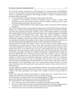
Fig. 1. The governing equations consist of field equations (conservations of mass, momentum
and energy) and constitutive equations. The constitutive equations distinguish classical fluid
mechanics from non-Newtonian fluid mechanics, due to Newton’s viscosity law is valid for
all flow situations (the viscosity is constant at any shear rate) and all Newtonian viscous
fluids, but not for non-Newtonian fluids, for which their viscosities depend on the flow
conditions (I2 is the second invariant of the tensor of shear rates) among other parameters.

Independently on whether the problem is isothermal or not, the viscosity relates the stress
to the motion of the continuum. This equation for non-Newtonian fluids is also known as
rheological equation of state. Whereas the field equations are the same for all materials,
constitutive equation will in general vary from one non-Newtonian material to another,


4
6

Numerical Simulations, Applications, Examples and Theory
Numerical Simulations - Examples and Applications in Computational Fluid Dynamics

and possibly from one type of flow to another. It is this last point which distinguishes
non-Newtonian fluid mechanics from classical fluid mechanics, where the use of Newton’s
viscosity law gives rise to the Navier-Stokes equations, which are valid for all Newtonian
viscous fluids (Crochet et al., 1985). Figure 1 shows a sketch of the governing equations.
Finally, it will be also needed to define initial and boundary conditions in order to solve the
specific problems.
2.1.1 Field equations for steady flow in pipes with circular cross-section

Independently on the constitutive equation, the stress tensor (τ) can be assumed as the sum
of hydrostatic pressure, corresponding to a static state of the fluid (− pI), and the viscous
stresses (τ ), which represent the dynamic part of the stress tensor. In 1845, Stokes deduced
a constitutive viscosity equation (Equation 3) generalizing Newton’s idea, which is valid for
many fluids, known as Newtonian fluids:
˙
τ = A : γ,

(3)

˙
where A is a forth order tensor generally depending on time, position and velocity, and γ the
deformation rate tensor2 . For newtonian fluids, A does not depend on velocity. Those fluids
not accomplishing the Equation 3 are known as Non-Newtonian Fluids.
In the particular case of having an isotropic fluid, the Equation 3 simplifies considerably in
Equation 4
1
1
∇v + ∇v T − ∇ · vI + ηv ∇ · vI,
(4)
2
3
where η is the viscosity associated to the pure shear deformation of the fluid, and ηv is the
volumetric viscosity coefficient and it is related to the volumetric deformation of the fluid
due to normal forces. Then, for an isotropic fluid, the Navier-Stokes equation is obtained by
introducing the Equation 4 in the Equation 2.
τ = 2η

∂ρv
+ ∇ · (ρvv) = −∇ p + ∇ · η ∇v + ∇v T
∂t

+∇

2
ηv − η ∇ · v + ρ f m .
3

(5)

Moreover, if the fluid can be considered incompressible (ρ = cte), the equation of continuity
reduces to Equation 6

∇ · v = 0,

(6)

and, consequently, the Equation 5 simplifies reaching the form given by Equation 7
ρ

∂v
+ v · ∇v
∂t

= −∇ p + ∇ · η ∇v + ∇v T

+ ρ fm .

(7)

Reached this point, it is worth to point out that these reduced expressions of field equations
(Equations 6 and 7) are only valid for an isotropic and incompressible fluid in isothermal
conditions. It is now the moment of considering the simplifications of the field equations
due to the facts that the fluid is flowing here in laminar steady state through an horizontal
cross-section pipe (Figure 2).
2 Also

˙
known as the rate-of-strain tensor: γ = ∇v + ∇v T .

Numerical Simulation in Steady flow of
Non-Newtonian Fluids in Pipes with Circular Cross-SectionFluids in Pipes with Circular Cross-Section
Numerical Simulation in Steady flow of Non-Newtonian

5
7

Fig. 2. Skecth of a pipe with lenght L and diameter D << L. The coordinates system here
considered is cylindrical and its origin is placed and centered at the entrance of the pipe.
This is a canonical problem in Fluid Mechanics. The unidirectional and steady flow of a fluid
∂( p+ρU )

through this pipe is originated by a constant gradient of reduced pressure pl = − ∂z
=
cte, where U is a potential from which all massive forces derivate ( f m = −∇U) and z is the
axial coordinate. It can be proved that the laminar and fully developed flow in a pipe is
axysymmetric, i.e. there are not dependences with the azimuthal coordinate (eθ ). Moreover,
the r-component of vector v is zero. From the continuity equation (Equation 6), it can be
derived that dvz = 0 and, consequently, the velocity vector expressed in cylindrical coordinates
dz
is given by Equation 8
v = ( vr , v θ , v z ) = v z ez ,
with vz = vz

(r )3

(8)

Then, the deformation rate tensor is given by Equation 9

⎛

∇v + ∇vT = ⎝
and, subsequently, the term ∇ · η
given by Equation 10

0
0

dvz
dr
∇v + ∇v T

dvz
dr

0
0
0

0
0

⎠,

(9)

in Equation 7 is reduced to the expression

⎛

∇ · η ∇v + ∇vT

⎞

⎜
=⎝

0
0
1 d
r dr

rη dvz
dr

⎞
⎟
⎠.

(10)

In this way, the field equations are reduced to a second order ordinary differential equation
(Equation 11) (Landau & Lifshitz, 1987). It must be noticed that this equation is needed to be
completed with two boundary conditions and a constitutive equation, but not initial condition
because the flow is steady.
pl +

1 d
r dr

rη

dvz
dr

=0

(11)

3 This dependence can be deduced from the fact that, while v is zero at r = D/2 by the no-slip
z
condition, in other r-value is that sure vz is non-zero.


6
8

Numerical Simulations, Applications, Examples and Theory
Numerical Simulations - Examples and Applications in Computational Fluid Dynamics

2.1.2 Boundary conditions

For a Newtonian fluid, the constitutive equation for the viscosity does not depend on the flow
conditions and it is simply a constant coefficient η = cte. Therefore, the Equation 11 is linear
and its general solution is given by Equation 12, where the values of the constants C1 and C2
will depend on the boundary conditions.
v z (r ) = −

pl r2

+ C1 lnr + C2
4η

(12)

Classically, in Fluid Mechanics, these boundary conditions consists of the following ones:
– The no-slip condition holds that the particles of fluid adjacent to the wall of the pipe move
with the wall velocity (Equation 13)
vz (r = D/2) = 0.

(13)

– The no-singularity condition consists of assuming that vz is a continuous function and
its first derivative exists and is also continuous, therefore the Equation 14 must be
accomplished
dvz
(14)
(r = 0) = 0.
dr
Then, the Equation 12 reduces to Equation 15, i.e. the velocity profile for a Newtonian,
isotropic and incompressible fluid under laminar and steady flow through a circular
cross-section pipe is parabolic, as studied experimentally by Hagen in 1839 and Poiseuille
in 1840 (Papanastasiou et al., 2000).
v z (r ) =

pl
4η

D2
− r2

4

(15)

However, when it is considered the laminar steady flow of a non-Newtonian fluid through
this kind of pipes things change. Even though the no-singularity boundary condition still
holds, the assumption of the no-slip condition is not as straightforward as it might seem.
Rheologists have, for good reasons, been more concerned about the validity of the concept
than workers in Newtonian fluid mechanics. With the benefit of decades of both theoretical
and experimental interest, it is possible to assess that at least three factors are of importance
concerning slip (Tanner & Walters, 1998):
– No effective slip can occur when molecular size is smaller than the wall roughness scale.
– For large molecules, relative to the wall roughness scale, the temperature and chemical
adherence properties may be of great significance in setting the critical shear stress at which
slip occurs.
– Normal pressure may assist in reducing slip.
Taking these factors about the slip at the wall into account, we will however assume that the
no-slip boundary condition holds in all the cases here considered.


Numerical Simulation in Steady flow of
Non-Newtonian Fluids in Pipes with Circular Cross-SectionFluids in Pipes with Circular Cross-Section
Numerical Simulation in Steady flow of Non-Newtonian

7
9

2.1.3 Constitutive equations for non-newtonian fluids

Constitutive equations (or rheological equations of state) are equations relating suitably

defined stress and deformation variables (Barnes et al., 1993). The simplest example is the
constitutive law for the Newtonian viscous liquid (Equation16), where a constant viscosity
coefficient is sufficient to determine the behaviour of incompressible Newtonian liquids under
any conditions of motion and stress. The measurement of this viscosity coefficient involves
the use of a viscometer, defined simply as an instrument for the measurement of viscosity.
˙
τ = ηγ

(16)

However, as the viscosity of non-Newtonian liquids may be dependent on the flow conditions,
i.e. the rate-of-strain tensor, the viscometer is therefore inadequate to characterize the
behaviour of these materials and has to be replaced by a rheometer, defined as an instrument
for measuring rheological properties. One of the objectives of Rheometry is to assist in the
construction of rheological equations of state (Walters, 1975).
If non-Newtonian viscosity, a scalar, is dependent on the rate-of-strain tensor, then it must
depend only on those particular combination of components of the tensor that are not
dependent on the coordinate system, the invariants of the tensor (Bird et al., 1987):
˙
– I1 = ∑3=1 γii .
i
˙ ˙
– I2 = ∑3=1 ∑3=1 γij γ ji .
i
j
˙ ˙ ˙
– I3 = ∑3=1 ∑3=1 ∑3=1 γij γ jk γki .
i
j
k

It can be deduced with ease that I1 = 0 for an incompressible fluid. In addition, I3 turns
out to be zero for shearing flows. Hence, for the flow problems here considered, η is solely
˙
dependent on I2 . Actually, it is preferred to use γ, the magnitude of the rate-of-strain tensor
˙
(γ), instead of I2 , being both parameters related by the Equation 17 (Macosko, 1994)
˙
γ=

1 3 3
˙ ˙
γ γ =
2 i∑ j∑ ij ji
=1 =1

1
I .
2 2

(17)

As this chapter is devoted to the steady flow of non-Newtonian fluids in pipes with circular
cross-section, which is a kind of flow dominated by shear viscosity and where the elasticity of
the fluid has no considerable repercussions, the most suitable constitutive equation is given
by the Generalized Newtonian Model (GNM) given by Equation 18. This is an inelastic model
for which the extra stress tensor is proportional to the strain rate tensor, but the “constant”
of proportionality (the viscosity) is allowed to depend on the strain rate. The inelastic model
possesses neither memory nor elasticity, and therefore it is unsuitable for transient flows, or
flows that calls for elastic effects (Phan-Thien, 2002).
˙ ˙

τ = η (γ) γ

(18)

Consequently, Equation 11 can be rewritten for non-Newtonian liquids as Equation 19
pl +

1 d
r dr

˙
rη (γ)

dvz
dr

= 0.

(19)

˙
The GNM is quite general because the functional form of η (γ) is not specified. It must be
given or fit the data to predict the flow properties. We will introduce different models for


8
10

Numerical Simulations, Applications, Examples and Theory
Numerical Simulations - Examples and Applications in Computational Fluid Dynamics

˙
η (γ), but many other functional forms can be used and these can be found in the literature or
in flow simulation softwares. Before that, it is important to keep in mind the main limitations
of the GNM (Morrison, 2001):
– They rely on the modeling shear viscosity to incorporate non-Newtonian effects, and
therefore it is not clear whether these models will be useful in nonshearing conditions.
– They do not predict shear normal stresses N1 and N2 , which are elastic effects, and therefore
they can not consider memory effects.
Nevertheless, the GNM enjoys success in predicting pressure-drop versus flow curves for
steady flow of non-Newtonian fluids in pipes with circular cross-section.
˙
As it has been mentioned above, it is possible to obtain η (γ) by means of experiments carried
out in a rheometer. In a shear rheometer, the material is undergone to simple shear conditions,
for which the rate-of-strain tensor is given by the Equation 20
⎞
⎛
0
0
0
⎜
dvθ ⎟
0
˙
(20)
γ = ∇v + ∇vT ∼ ⎝ 0
=
dz ⎠ ,
dvθ
0

0
dz
whose invariants are the following ones:
˙
– I1 = tr γ = 0
– I2 = 2

dvθ
dz

2

˙
– I3 = det γ = 0
In the case of a steady flow in pipes with circular cross-section, the rate-of-strain tensor is
given by the Equation 9 and its invariants are the following ones:
˙
– I1 = tr γ = 0
– I2 = 2

dvz
dr

2

˙
– I3 = det γ = 0
It can be observed that in both flow conditions the fluid is undergone to simple shear and
|I |

dvθ
dvz
2
˙
it can be stated that γ =
2 = | dz | = | dr |. Then, the shear dependence of the viscosity
in steady state observed in the rheological experiments could be used directly in Equation
19. It has been already probed that the experimental data obtained with a rheometer can be
used successfully for the prediction of the transport characteristic in pipelines (Masalova et al.,
2003).

2.1.3.1 GNM for shear thinning fluids

Most of non-Newtonian fluids (foods, biofluids, personal care products and polymers)
undergone to steady shear exhibit shear thinnning behavior, i.e. their viscosity decreases
with increasing shear rates. During flow, these materials may exhibit three distinct regions
(see Figure 3): a lower Newtonian region where the apparent viscosity (η0 ), usually called the
limiting viscosity at zero shear rate, is constant with changing shear rates; a middle region
where the apparent viscosity is decreasing with shear rate and the power law equation is


Numerical Simulation in Steady flow of
Non-Newtonian Fluids in Pipes with Circular Cross-SectionFluids in Pipes with Circular Cross-Section
Numerical Simulation in Steady flow of Non-Newtonian

9
11

a suitable model for this region; and an upper Newtonian region where the viscosity (η∞ ),
called the limiting viscosity at infinite shear rate, is constant with changing shear rates (Steffe,

1996). Sometimes the position of the typical behaviour along the shear-rate axis is such
that the particular measurement range used is either too low or too high to pick up the
higher-shear-rate part of the curve4 .

Fig. 3. Typical viscosity curve for a shear thinning behaviour containing the three regions:
The two limiting Newtonian viscosities, η0 and η∞ , separated by a shear thinning region.
˙
One equation for η (γ) that describes the whole shear thinning curve is called the Cross model,
named after Malcolm Cross, a rheologist who worked on dye-stuff and pigment dispersions.
He found that the viscosity of many suspensions could be described by the equation of the
form given by Equation 21
η0 − η ∞
,
(21)
˙
1 + (K γ)m
where K has the dimensions of time, and m is dimensionless. The degree of shear thinning is
dictated by the value of m, with m tending to zero describes more Newtonian liquids, while the
most shear-thinning liquids have a value of m tending to unity. If we make various simplifying
assumptions, it is not difficult to show that the Cross equation can be reduced to Sisko5 or
power-law models6 . The Carreau model is very similar to the Cross model (Equation 22)
˙
η ( γ ) = η∞ +

˙
η ( γ ) = η∞ +

η0 − η ∞
˙
1 + ( K γ )2

m/2

,

(22)

both (Cross and Carreau equations) are the same at very low and very high shear rates, and
˙
only differ slightly at K γ ≈ 1 (Barnes, 2000).
The use of Cross or Carreau models in the Equation 19 results in a differential equation that
can not be solved analytically and, thefore, numerical techniques are needed.
It is worth to emphasize here that due to the boundary condition of no-singularity imposed at
the axis of symmetry, it is highly important choosing a model which contains what happens
to the viscosity at low shear rates in order to solve this problem.
that the typical shear-rate range of most laboratory viscometers is between 10−2 and 103 s−1
the viscosity is just coming out of the power-law region of the flow curve and flattening off
˙
˙
towards η∞ , the Sisko model is the best fitting equation: η (γ) = η∞ + k γn−1 .
6 In many situations, η >> η , K γ >> 1, and η is small. Then the Cross equation (with a simple
˙
∞
∞
0
change of the variables K and m) reduces to the well-known power-law (or Ostwald-de Waele) model,
˙
˙
which is given by η (γ) = kγn−1 , where k is called the consistency and n the power-law index.
4 Note

5 When


10
12

Numerical Simulations, Applications, Examples and Theory
Numerical Simulations - Examples and Applications in Computational Fluid Dynamics

2.1.3.2 GNM for shear thickening fluids

Shear thickening is defined in the British Standard Rheological Nomenclature as the increase
of viscosity with increase in shear rate (Barnes, 1989). This increase in the effective viscosity
occurs when the increasing shear rate exceeds a certain critical value. Although shear
thickening fluids (STFs) are much less common than shear thinning materials in industry,
an increasing number of applications take advantage of the shear thickening behaviour to
improve their performance, i.e. the incorporation of STFs to Kevlar R fabrics in order to
improve the ballistic protection (Lee et al., 2003; Kirkwood et al., 2004) and enhance stab
resistance (Decker et al., 2007). However, shear thickening is an undesirable behaviour in
many other cases and it should never be ignored, because this could lead to technical problems
and even to the destruction of equipment, i.e. pumps or stirrers (Mezger, 2002).
Figure 4 shows the viscosity curve of a STF containing the three characteristic regions typically
exhibited: slight shear thinning at low shear rates, followed by a sharp viscosity increase over
a threshold shear rate value (critical shear rate), and a subsequent pronounced shear thinning
region at high shear rates. Nowadays, the physics of the phenomenon is deeply understood
thanks to the use of modern rheometers, scattering techniques, rheo-optical devices and
Stokesian dynamic simulations (Bender & Wagner, 1996; Hoffman, 1974; Boersma et al., 1992;
D’Haene et al., 1993; Hoffman, 1998; Maranzano & Wagner, 2002; Larson, 1999). However,
there is a lack of experimental or theoretical models able to predict the whole effective

viscosity curve of STFs, including the shear thinning behaviours normally present in these
materials for low enough and high enough values of the shear rate.

Fig. 4. Typical viscosity curve for a shear thickening behaviour containing the three regions:
The two limiting shear thinning behaviours separated by a shear thickening region.
As it has been mentioned above, many functional forms have been proposed in the past for
˙
η (γ) in the case of shear thinning fluids. In contrast, for shear thickening fluids only the
power-law model, given by (Equation 23), has been commonly used
˙
˙
η ( γ ) = k γ n −1 .

(23)

Its major drawback is that power-law model can only fit the interval of shear rates where the
viscosity increases with the shear rate n > 1, but it fails to describe the low and the high shear
rate regions (Macosko, 1994), where shear-thinning behaviours are normally observed.
Very recently, Galindo-Rosales et al. (2010) have provided a viscosity function for shear
thickening behavior able to cover these three characteristic regions of the general viscosity
curve exhibited by STF. It consists in using a piecewise definition, taking the three different


Numerical Simulation in Steady flow of
Non-Newtonian Fluids in Pipes with Circular Cross-SectionFluids in Pipes with Circular Cross-Section
Numerical Simulation in Steady flow of Non-Newtonian

11
13

regions into account separately. According to this approach, they have defined the viscosity
function as follows,
⎧
˙
˙
˙
for γ ≤ γc ,
⎨ η I (γ)
˙
˙
˙
˙
˙
η I I (γ) for γc < γ ≤ γmax ,
η (γ) =
(24)
⎩
˙
˙
˙
η I I I (γ) for γmax < γ,
˙
where ηi (γ) is the viscosity function that fits the zone i of the general viscosity curve (for
i = I, I I, I I I). As it was pointed out by Souza-Mendes & Dutra (2004), the functions ηi
must be chosen such that both, the composite function given by Equation 24, as well as
˙
its derivative with respect to γ, are continuous. This procedure avoids practical problems
in fitting procedures and in numerical simulations. The viscosity function proposed in the
work of Galindo-Rosales et al. (2010), given by Equation 25, accomplishes these smoothness
requirements.

⎧
η0 − η c
⎪ η I ( γ ) = ηc +
˙
˙
˙
for γ ≤ γc ,
nI
⎪
˙
γ2
⎪
1 + K I γ − γc
⎪
˙ ˙
⎪
⎪
⎪
⎪
⎨
ηc −ηmax
˙
˙
˙
˙
for γc < γ ≤ γmax ,
η (γ) = ηmax +
˙
η (γ) =
(25)

nI I
˙ ˙
γ γc
⎪ II
˙
1+ K I I γ−−max γ
⎪
˙ γ
˙
⎪
⎪
⎪
⎪
⎪
⎪
ηmax
⎩ η I I I (γ) =
˙
˙
˙
for γmax < γ.
˙ ˙
1+[K (γ−γ )]n I I I
III

max

It must be noticed that the parameters appearing in the branches of Equation 25 have the
same dimensions and interpretation than those analogous for the Cross model (Equation 21):
Ki (for i = I, I I, I I I) possess dimension of time and are responsible for the transitions between

the plateaus and the power-law, while the dimensionless exponents ni are related to the slopes
of the power-law regimes. Equation 25 is able to capture the three regimes characteristic of
STF materials.
˙
Then, substituting any the form of η (γ) given in Equation 25 in the Equation 19 will results in
a differential equation that can not be solved analytically and, thefore, numerical techniques
will be needed again.

3. Numerical simulations
Classical Fluid Mechanics offers a wide variety of possibilities with regards to numerical
algorithms based on finite elements, finite volume, finite differences and spectral methods
(Wesseling, 2001). Computational rheologists do not have a recipe which lets them know
which one is more suitable to work with in each particular problem, although most of the
published works related to solve 2-D problems in steady state are based on finite element
methods (Keunings, 1999). However, it has been proved that finite volume methods produce
better results (O’Callaghan et al., 2003) due mainly to a good conservation of the fluid
properties (mass, momentum and energy) and they allow to discretize complex computational
domain in a simpler way (Fletcher, 2005).
The problem considered here, because of its geometrical features, can be solved by any of
the numerical techniques already mentioned, although we have finally used the finite volume
technique (Pinho & Oliveira, 2001; Pinho, 2001). As the flow problem is axysymmetric, the
volume domain can be simplified to a 2-D domain with a length7 (L = 2 m) and a width
7 Its

lenght is long enough to ensure that the regime of fully developed flow is reached.


12
14

Numerical Simulations, Applications, Examples and Theory
Numerical Simulations - Examples and Applications in Computational Fluid Dynamics

(D = 1 cm << L). This domain is meshed by rectangles in a structured grid: in z-axis from
the inlet (ratio 1.05 and 500 nodes) and r-axis from the axis (ratio 1.0125 and 50 nodes), which
has been validated by correlating the analytical and numerical results given for the case of a
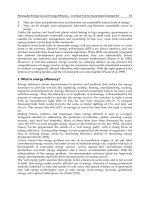
Newtonian fluid (Figure 5).

(a)

(b)

Fig. 5. (a) Horizontal pipeline with L >> R in order to ensure that the flow reaches the fully
developed region. (b) Validation of the grid by means of the comparison between the
numerical result and the analytical solution of the fully developed velocity profile for a
Newtonian liquid.
As a consequence of the friction drag, there is a pressure drop. The energy required to
compensate the dissipation due to frictional losses against the inside wall and to keep the fluid
moving is usually supported by a pump. A large amount of data obtained experimentally for
many different Newtonian fluids in pipes having diameters differing by orders of magnitude
and roughness have been assembled into the so-called friction-factor chart or Moody chart,
relating the friction factor with Reynolds number in laminar and turbulent regime and relative
roughness. In laminar flow, the friction factor does not depend on the roughness of the inner
surface of the pipe and can be calculated by the Equation 26
16
,
(26)
Re
where f is the friction factor and Re is the Reynolds number. Nevertheless, when the fluid is
non Newtonian, the Moody chart and the Equation 26 are useless due to in non-Newtonian

fluids there is an extra dissipation of energy expent in modifying the internal structure of
the fluid8 . It then is needed to analyse the particular flow behaviour of the fluid considered,
obtain its constitutive equation and solve the momentum conservation equation in order to
characterize the steady flow in a pipe of circular cross-section.
As an example of how to proceed, two different non-Newtonian fluids (shear thinning and
˙
shear thickening fluids) are considered here. Firstly, their constitutive forms for η (γ) will be
obtained from their experimental viscosity curves. Secondly, the momentum conservation
equation in the steady state (Equation 19), considering axysimmetry and a cylindrical
coordinate system centered in the axis of the pipe, will be solved numerically by volume finite
methods. In order to have shear rates values within the limits of the experimental results
for each sample, the velocity inlet was always imposed at values below 0.1 m/s. Thus, the
f=

8 As it is oulined in the following subsection, the variations in the viscosity are due to variation in the
internal order of the fluid, which is possible thanks to the mechanical energy suplied by the shearing
motion.


Numerical Simulation in Steady flow of
Non-Newtonian Fluids in Pipes with Circular Cross-SectionFluids in Pipes with Circular Cross-Section
Numerical Simulation in Steady flow of Non-Newtonian

13
15

velocity profile, shear rate, apparent viscosity, pressure drop and friction factor were obtained
for each sample as function of velocity.
3.1 Experimental data set

Aerosil R fumed silica is a synthetic, amorphous and non-porous silicon dioxide produced
by Degussa A.G (Degussa, 1998) following a high temperature process. Aerosil R 200
presents a highly hydrophilic surface chemistry with surface silanol groups (Si − OH) that
can participate in hydrogen bonding. Because of the relatively high surface area (200m2 /g) of
these particles, the surface functional groups play a major role in the behavior of fumed silica
Degussa (2005a). In the unmodified state, the silanol group imparts a hydrophilic character to
the material. However, it is possible to modify its surface chemistry by means of a chemical
after treatment with silane. In this way, Aerosil R R805 is obtained from Aerosil R 200 particles
by replacing silanol groups with octadecylsilane chains, which results in an hydrophobic
behaviour of the particles (Degussa, 2005b).
The degree of network formation by fumed silica in a liquid depends on the concentration of
solid and type (hydrophilic versus hydrophobic) of silica, as well as the nature (polarity) of the
suspending medium. Therefore, these three main factors allow to the suspensions of Aerosil R
fumed silica inside a fluid possess a variety of rheological behaviors (Khan & Zoeller, 1993;
Raghavan & Khan, 1995). This variety of rheological behaviors makes silica particle a very
interesting filler from the point of view of a wide range of applications. For example, gels
of fumed silica in mineral or silicone oils are used as filling compounds in fiber-optic cables,
while in polyethylene glycols are being considered for application as polymer electrolytes in
rechargeable lithium batteries(J´ uregui Beloqui & Martin Martinez, 1999; Dolz et al., 2000;
a
Walls et al., 2000; Li et al., 2002; Fischer et al., 2006; Yziquel et al., 1999; Ouyang et al., 2006).
It has been already reported elsewhere (Galindo-Rosales & Rubio-Hern´ ndez, 2007; 2010)
a
that suspensions of Aerosil R R805 and Aerosil R 200 in Polypropylene Glycol (PPG) with
a molecular weight of 400 g/mol exhibit completely different rheological behaviour. PPG
molecules interfere in the formation of the fumed silica network by attaching itself to the
active Si − OH sited on the silica surface. Therefore no bridging between silica particles
occurs with polar solvents, such as polypropylene glycol, that have a stronger affinity for
fumed silica than that existing between two fumed silica. The solvent attaches itself to the
surface silanol group of the fumed silica rendering it inactive for further network formation.

For that reason, when dispersing Aerosil R 200 in polypropylene glycol, it is expected that
primary aggregates interconnect, originating flocs with different sizes depending on the
weight fraction. On the contrary, a large interconnection between the flocs, which may result
in a three dimensional structure, should not take place. Therefore, the suspension would be
non-flocculated (Raghavan & Khan, 1997; Raghavan et al., 2000). However the presence of
octadecylsilane chemical bonds on the surface of Aerosil R R805 avoids that PPG molecules
attached to the silica particles and lets them develop a three dimensional network without
interacting chemically with polypropylene gycol chains. So a flocculated suspension is formed
(Khan & Zoeller, 1993).
The steady viscosity curves, shown in Figure 6, represent the steady viscosity reached by
the suspensions at different values of shear rates. Therefore, the shape of these curves is
a consequence of the order achieved by silica particles inside the polymer matrix under flow
conditions. According to the previous analysis, Aerosil R R805 suspension is flocculated after a
long time at rest, and the network breaks down when subjected to shear, a behavior known as
shear thinning. Figure 6 confirms that the higher the shear rate applied, the lower the apparent