Valuing Employee Stock Options Part 5 doc
Bạn đang xem bản rút gọn của tài liệu. Xem và tải ngay bản đầy đủ của tài liệu tại đây (322.04 KB, 14 trang )
CHAPTER
5
Applicability of
Monte Carlo Simulation
INTRODUCTION TO THE ANALYSIS
Analyses in previous chapters clearly indicate that using the BSM alone is
insufficient to measure the true fair-market value of ESOs. Option pricing
has made vast strides since 1973 when Fischer Black and Myron Scholes
published their path-breaking paper providing a model for valuing Euro-
pean options. While Black and Scholes’ derivations are mathematically
complex, other approaches broached in this book, namely those using
Monte Carlo simulation and binomial lattices, provide much simpler appli-
cations but at the same time enable a similar wellspring of information.
1
In
fact, applying binomial lattices with Monte Carlo simulation has been
made much easier with the use of software and spreadsheets.
This chapter focuses on the applicability of Monte Carlo simulation as
it pertains to valuing stock options and as a means of simulating the inputs
that go into a customized binomial lattice—that is, used in conjunction
with binomial lattices. This chapter begins with a brief review of the three
types of option pricing methodologies and continues with a quantitative as-
sessment of their analytical robustness under different conditions. The sim-
ulation approach to valuing options will be shown to be precise when it
comes to valuing simple European options without dividends. In contrast,
when it comes to American or mixed options with exotic features (vesting,
forfeiture, suboptimal behavior, and blackout dates), the simulation ap-
proach to valuing options breaks down and cannot be used. The binomial
lattice is a much better candidate when these exotic elements exist. How-
ever, Monte Carlo simulation still proves to be a powerful and useful tool
for simulating the uncertain input variables with correlations, and allows
tens of thousands of scenarios to enter into a customized binomial lattice. It
is shown later in this chapter that a precision-controlled simulation can in-
51
ccc_mun_ch05_51-64.qxd 8/20/04 9:21 AM Page 51
crease the confidence of the results and narrow the errors to less than a
$0.01 precision with a 99.9 percent statistical confidence level, increasing
the confidence of the valuation results.
In the rest of the chapter a brief review of the three mainstream ap-
proaches is made and the valuation results are then compared. The simula-
tion approach to valuation will be shown not to be applicable by itself; but
when coupled with the customized binomial lattices, it provides a powerful
analytical tool that yields robust results.
The Black-Scholes Model
In order to fully understand and use the BSM, one needs to understand the
assumptions under which the model was constructed. These are essentially
the caveats that go into using the BSM option pricing model. These as-
sumptions are violated quite often, but the model still holds up to scrutiny
when applied appropriately to European options. A European option is the
type of option that can be exercised only on its expiration date and not be-
fore. In contrast, most executive stock options awarded are American op-
tions, where the holder of the option is allowed to exercise at any time
(except on blackout dates) once the award has been fully vested.
The main assumption that goes into the BSM is that the underlying as-
set’s price structure follows a Brownian Motion with static drift and
volatility parameters, and that this motion follows a Markov-Weiner sto-
chastic process. In other words, it assumes that the returns on the stock
prices follow a lognormal distribution. The other assumptions are fairly
standard, including a fair and timely efficient market with no riskless arbi-
trage opportunities, no transaction costs, and no taxes. Price changes are
also assumed to be continuous and instantaneous. Finally, the risk-free rate
and volatility are assumed to be constant throughout the life of the option,
and the stock pays no dividends.
2
However, for fairness of comparison, a
modification of the BSM is used—the GBM. This modification allows the
incorporation of dividends in a standard European option.
Monte Carlo Path Simulation
Monte Carlo simulation can be easily adapted for use in an options valua-
tion paradigm. There are multiple uses of Monte Carlo simulation includ-
ing its use in risk analysis and forecasting. Here, the discussion focuses on
two distinct applications of Monte Carlo simulation: solving a stock op-
tion valuation problem versus obtaining a range of solved option values.
Although these two approaches are discussed separately, they can be used
together in an analysis.
52 IMPACTS OF THE NEW FAS 123 METHODOLOGY
ccc_mun_ch05_51-64.qxd 8/20/04 9:21 AM Page 52
Applying Monte Carlo Simulation
to Obtain a Stock Options Value
Monte Carlo simulation can be applied to solve an options valuation prob-
lem, that is, to obtain a fair-market value of the stock option. Recall that
the mainstream approaches in solving options problems are the binomial
approach, closed-form equations, and simulation. In the simulation ap-
proach, a series of forecast stock prices are created using the Brownian
Motion stochastic process, and the option maximization calculation is ap-
plied to the series’ end nodes, and discounted back to time zero, at the risk-
free rate.
Note that simulation can be easily used to solve European-type op-
tions, but it is fairly difficult to apply simulation to solve American-type
options.
3
In fact, certain academic texts list Monte Carlo simulation’s
major limitation as that it can be used to solve only European-type op-
tions.
4
If the number of simulation trials are adequately increased, cou-
pled with an increase in the simulation time-steps, the results stemming
from Monte Carlo simulation also approach the BSM value for a Euro-
pean option.
Binomial Lattices
Binomial lattices, in contrast, are easy to implement and easy to explain.
They are also highly flexible, but require significant computing power and
lattice steps to obtain good approximations, as will be seen in the next
chapter. The results from closed-form solutions can be used in conjunction
with the binomial lattice approach when presenting a complete stock op-
tions valuation solution. Binomial lattices are particularly useful in captur-
ing the effect of early exercise as in an American option with dividends,
vesting and blackout periods, suboptimal early exercise behaviors, forfei-
tures, performance-based vesting, changing volatilities and business envi-
ronments, changing dividend yield, changing risk-free rates, and so
forth—the same real-life conditions that cannot be accounted for in the
BSM, GBM, or simulation. Binomial lattices can even account for exotic
events such as stock price barriers (a barrier option exists when the stock
option becomes either in-the-money or out-of-the-money only when it hits
a stock price barrier), vesting tranches (a specific percent of the options
granted becomes vested or exercisable each year, or that senior manage-
ment has different option grants than regular employees), and so forth.
Monte Carlo simulation can then be applied to simulate the probabilities
of forfeitures and underperformance of the firm, and use these as the in-
puts into the binomial lattices.
5
Applicability of Monte Carlo Simulation 53
ccc_mun_ch05_51-64.qxd 8/20/04 9:21 AM Page 53
Analytical Comparison
The following presents a results comparison of the three methods dis-
cussed. The main goal of the analysis is to show that under certain restric-
tive conditions, all three methodologies provide identical results, indicating
that all three methods are robust and correct. However, when conditions
are changed to mirror real-life scenarios, binomial lattices provide a much
more accurate fair-value assessment than the GBM and BSM approaches,
where the latter approaches may sometimes overvalue and at other times
undervalue the ESO.
Figure 5.1 illustrates a comparative analysis of the three different op-
tions valuation methodologies for a simple set of inputs. The usual inputs
in the options valuation model are: expiration in years, stock price, volatil-
ity, risk-free rate, dividend rate, and strike price. Notice that with a simple
set of inputs where the stock is assumed not to pay any dividends, the bi-
nomial approach with 5,000 steps yields $39.43, identical to the BSM of
$39.43. The path simulation approach also yields a value of $39.43.
6
No-
tice in addition, that the American closed-form model results indicate iden-
tical values when no dividend payments exist, and that all methods yield
the same values in a European option. In American options when a divi-
dend exists, the values obtained from the three methodologies are vastly
different, as seen in Table 5.1 (a–d).
When a dividend yield exists, that is, when the underlying firm’s stocks
pay dividends, the results from a BSM or GBM are no longer robust or
correct, because early execution is optimal, making the stock option, an
American-type option, more valuable than is estimated using the BSM.
Table 5.1 (a–d) illustrates this point. For instance, panel (a) of Table 5.1
shows the results from a BSM, and panel (b) is the binomial lattice for a
European option, while the panel (c) shows the results from an American
closed-form approximation model, and panel (d) shows the binomial ap-
proach for an American option. Notice that for all four panels, the first
column results are identical when no dividends exist. This indicates that all
four methodologies are robust and consistent and provide identical values
at the limit, under the condition of no dividends and are all valid for Euro-
pean-type options. However, when dividends exist, the BSM breaks down
and is no longer valid, especially when the option is of the American type.
Applying Monte Carlo Simulation for
Statistical Confidence and Precision Control
Alternatively, Monte Carlo simulation can be applied to obtain a range of
calculated stock option fair values. That is, any of the inputs into the stock
54 IMPACTS OF THE NEW FAS 123 METHODOLOGY
ccc_mun_ch05_51-64.qxd 8/20/04 9:21 AM Page 54
FIGURE 5.1 Comparing the three approaches.
Comparing Approaches
Input Parameters
Expiration in Years 5.00
Volatility 35.00%
Initial Stock Price $100.00
Risk-Free Rate 5.00%
Dividend Rate 0.00%
Strike Cost $100.00
European Option Results
Binomial Approach $39.43
Black-Scholes Model $39.43
Path-Dependent Simulation $39.43
Generalized Black-Scholes $39.43
American Option Results
Binomial Approach $39.43
Black-Scholes Model N/A
Path Dependent Simulation N/A
Closed-Form Approximation Model $39.43
Simulation Calculation
Simulate Value 0.00
Payoff Function 19.47
Binomial Steps 5,000 Steps ▼ Binomial Steps 5,000 Steps ▼
Time Simulate Steps Value Value (2) Time Simulate Steps Value Value (2) Time Simulate Steps Value
0 0.00 0.00 100.00 100.00 21 –0.05 –0.09 82.87 86.17 42 –1.30 –3.87 35.01
1 –0.59 –4.40 95.60 95.60 22 0.24 1.78 84.65 88.32 43 –1.27 –3.40 31.61
2 –0.85 –6.14 89.46 89.18 23 –2.00 –13.05 71.61 72.91 44 1.13 2.88 34.48
3 1.23 8.81 98.28 99.03 24 –0.66 –3.49 68.11 68.03 45 –0.29 –0.70 33.79
4 –0.62 –4.56 93.72 94.39 25 1.20 6.57 74.68 77.68 46 1.34 3.64 37.42
5 0.94 7.14 100.85 102.01 26 –1.59 –9.13 65.55 65.45 47 0.43 1.34 38.77
6 0.84 6.92 107.77 108.87 27 –0.54 –2.59 62.96 61.49 48 0.17 0.61 39.38
7 –1.17 –9.60 98.17 99.96 28 –1.38 –6.65 56.30 50.92 49 –0.69 –2.03 37.35
8 –1.02 –7.62 90.55 92.20 29 –1.50 –6.48 49.83 39.42 50 –0.78 –2.19 35.16
9 –0.09 –0.40 90.15 91.76 30 0.20 0.89 50.71 41.20 51 0.62 1.79 36.95
10 –0.66 –4.40 85.76 86.88 31 0.24 1.06 51.78 43.30 52 –1.64 –4.66 32.29
11 –0.99 –6.45 79.30 79.36 32 –1.65 –6.55 45.23 30.64 53 –0.68 –1.64 30.65
12 0.35 2.36 81.66 82.33 33 –0.88 –2.99 42.23 24.03 54 –1.90 –4.48 26.17
13 2.12 13.76 95.42 99.18 34 –1.29 –4.17 38.07 14.16 55 –0.52 –0.99 25.17
14 –0.27 –1.75 93.67 97.35 35 –0.50 –1.40 36.67 10.50 56 1.04 2.12 27.29
15 –1.49 –10.72 82.95 85.91 36 –0.26 –0.64 36.03 8.75 57 0.21 0.51 27.80
16 –0.57 –3.48 79.48 81.72 37 0.65 1.92 37.95 14.06 58 0.52 1.19 28.99
17 0.06 0.58 80.06 82.45 38 0.54 1.69 39.63 18.51 59 –0.78 –1.70 27.29
18 0.87 5.67 85.73 89.53 39 –0.57 –1.67 37.96 14.29 60 0.00 0.06 27.35
19 –0.34 –2.08 83.65 87.10 40 –0.42 –1.15 36.81 11.27 61 1.17 2.57 29.92
20 –0.14 –0.69 82.96 86.27 41 0.68 2.06 38.88 16.87 62 1.64 3.92 33.84
55
ccc_mun_ch05_51-64.qxd 8/20/04 9:21 AM Page 55
TABLE 5.1 (a–d) The Three Approaches’ Comparison Results
Black-Scholes Dividend Dividend Dividend Dividend Dividend Dividend Dividend Dividend Dividend Dividend Dividend
Model (0.00%) (1.00%) (2.00%) (3.00% (4.00%) (5.00%) (6.00%) (7.00%) (8.00%) (9.00%) (10.00%)
Years (1.00) $16.13 $16.13 $16.13 $16.13 $16.13 $16.13 $16.13 $16.13 $16.13 $16.13 $16.13 1
Years (2.00) $23.75 $23.75 $23.75 $23.75 $23.75 $23.75 $23.75 $23.75 $23.75 $23.75 $23.75 2
Years (3.00) $29.78 $29.78 $29.78 $29.78 $29.78 $29.78 $29.78 $29.78 $29.78 $29.78 $29.78 3
Years (4.00) $34.91 $34.91 $34.91 $34.91 $34.91 $34.91 $34.91 $34.91 $34.91 $34.91 $34.91 4
(a) Years (5.00) $39.43 $39.43 $39.43 $39.43 $39.43 $39.43 $39.43 $39.43 $39.43 $39.43 $39.43 5
Years (6.00) $43.47 $43.47 $43.47 $43.47 $43.47 $43.47 $43.47 $43.47 $43.47 $43.47 $43.47 6
Years (7.00) $47.14 $47.14 $47.14 $47.14 $47.14 $47.14 $47.14 $47.14 $47.14 $47.14 $47.14 7
Years (8.00) $50.48 $50.48 $50.48 $50.48 $50.48 $50.48 $50.48 $50.48 $50.48 $50.48 $50.48 8
Years (9.00) $53.55 $53.55 $53.55 $53.55 $53.55 $53.55 $53.55 $53.55 $53.55 $53.55 $53.55 9
Years (10.00) $56.39 $56.39 $56.39 $56.39 $56.39 $56.39 $56.39 $56.39 $56.39 $56.39 $56.39 10
1234567891011
Binomial
Approach Dividend Dividend Dividend Dividend Dividend Dividend Dividend Dividend Dividend Dividend Dividend
(European) (0.00%) (1.00%) (2.00%) (3.00%) (4.00%) (5.00%) (6.00%) (7.00%) (8.00%) (9.00%) (10.00%)
Years (1.00) $16.13 $15.51 $14.91 $14.33 $13.76 $13.21 $12.68 $12.16 $11.66 $11.17 $10.70 1
Years (2.00) $23.74 $22.42 $21.16 $19.95 $18.79 $17.69 $16.63 $15.62 $14.66 $13.74 $12.87 2
Years (3.00) $29.78 $27.71 $25.75 $23.90 $22.15 $20.50 $18.95 $17.49 $16.12 $14.84 $13.64 3
Years (4.00) $34.91 $32.06 $29.39 $26.89 $24.57 $22.40 $20.39 $18.53 $16.80 $15.21 $13.74 4
(b) Years (5.00) $39.43 $35.76 $32.37 $29.24 $26.36 $23.71 $21.27 $19.05 $17.01 $15.16 $13.48 5
Years (6.00) $43.47 $38.98 $34.87 $31.11 $27.69 $24.58 $21.76 $19.22 $16.92 $14.85 $13.00 6
Years (7.00) $47.13 $41.80 $36.97 $32.60 $28.66 $25.13 $21.96 $19.13 $16.62 $14.38 $12.40 7
Years (8.00) $50.48 $44.29 $38.74 $33.78 $29.36 $25.43 $21.95 $18.88 $16.17 $13.80 $11.74 8
Years (9.00) $53.55 $46.50 $40.25 $34.71 $29.82 $25.53 $21.77 $18.49 $15.63 $13.17 $11.04 9
Years (10.00) $56.38 $48.47 $41.52 $35.42 $30.10 $25.47 $21.46 $18.01 $15.04 $12.50 $10.33 10
1234567891011
56
ccc_mun_ch05_51-64.qxd 8/20/04 9:21 AM Page 56
TABLE 5.1 (a–d) (Continued)
Closed-Form
Approximation Dividend Dividend Dividend Dividend Dividend Dividend Dividend Dividend Dividend Dividend Dividend
(American) (0.00%) (1.00%) (2.00%) (3.00%) (4.00%) (5.00%) (6.00%) (7.00%) (8.00%) (9.00%) (10.00%)
Years (1.00) $16.13 $15.51 $14.91 $14.33 $13.79 $13.33 $12.88 $12.45 $12.05 $11.67 $11.31 1
Years (2.00) $23.75 $22.43 $21.16 $19.99 $18.96 $18.10 $17.26 $16.49 $15.77 $15.11 $14.49 2
Years (3.00) $29.78 $27.71 $25.77 $24.03 $22.58 $21.33 $20.16 $19.10 $18.12 $17.22 $16.40 3
Years (4.00) $34.91 $32.06 $29.45 $27.20 $25.37 $23.76 $22.30 $20.98 $19.78 $18.68 $17.69 4
(c) Years (5.00) $39.43 $35.77 $32.51 $29.80 $27.61 $25.67 $23.95 $22.40 $21.01 $19.75 $18.61 5
Years (6.00) $43.47 $39.00 $35.12 $31.99 $29.47 $27.23 $25.26 $23.52 $21.96 $20.56 $19.30 6
Years (7.00) $47.14 $41.84 $37.39 $33.86 $31.03 $28.51 $26.33 $24.42 $22.71 $21.19 $19.83 7
Years (8.00) $50.48 $44.37 $39.38 $35.48 $32.35 $29.58 $27.22 $25.15 $23.32 $21.69 $20.24 8
Years (9.00) $53.55 $46.64 $41.14 $36.90 $33.49 $30.49 $27.96 $25.75 $23.81 $22.09 $20.56 9
Years (10.00) $56.39 $48.69 $42.71 $38.15 $34.48 $31.27 $28.58 $26.25 $24.21 $22.41 $20.82 10
1234567891011
Binomial
Approach Dividend Dividend Dividend Dividend Dividend Dividend Dividend Dividend Dividend Dividend Dividend
(American) (0.00%) (0.00%) (0.00%) (0.00%) (0.00%) (0.00%) (0.00%) (0.00%) (0.00%) (0.00%) (0.00%)
Years (1.00) $16.13 $15.51 $14.91 $14.34 $13.83 $13.36 $12.93 $12.52 $12.14 $11.77 $11.42 1
Years (2.00) $23.74 $22.42 $21.17 $20.03 $19.05 $18.16 $17.35 $16.59 $15.89 $15.23 $14.61 2
Years (3.00) $29.78 $27.71 $25.79 $24.13 $22.70 $21.43 $20.27 $19.21 $18.24 $17.34 $16.51 3
Years (4.00) $34.91 $32.06 $29.50 $27.35 $25.50 $23.88 $22.42 $21.10 $19.89 $18.79 $17.79 4
(d) Years (5.00) $39.43 $35.78 $32.61 $29.98 $27.76 $25.81 $24.08 $22.52 $21.12 $19.86 $18.70 5
Years (6.00) $43.47 $39.02 $35.26 $32.19 $29.61 $27.37 $25.40 $23.64 $22.07 $20.66 $19.8 6
Years (7.00) $47.13 $41.88 $37.56 $34.08 $31.17 $28.66 $26.47 $24.54 $22.82 $21.28 $19.90 7
Years (8.00) $50.48 $44.42 $39.57 $35.71 $32.49 $29.74 $27.36 $25.26 $23.41 $21.77 $20.30 8
Years (9.00) $53.55 $46.70 $41.35 $37.12 $33.63 $30.66 $28.10 $25.86 $23.90 $22.16 $20.62 9
Years (10.00) $56.38 $48.76 $42.93 $38.36 $34.61 $31.44 $28.72 $26.36 $24.29 $22.48 $20.87 10
1234567891011
57
ccc_mun_ch05_51-64.qxd 8/20/04 9:21 AM Page 57
options valuation model can be chosen for Monte Carlo simulation if they
are uncertain and stochastic. Distributional assumptions are assigned to
these variables, and the resulting options values using the BSM, GBM, path
simulation, or binomial lattices are selected as forecast cells. These mod-
eled uncertainties include the probability of forfeiture and the employees’
suboptimal exercise behavior. The simulation examples throughout this
book use Decisioneering, Inc.’s Crystal Ball software.
The results of the simulation are essentially a distribution of the stock
option values. Keep in mind that the simulation application here is used to
vary the inputs to an options valuation model to obtain a range of results,
not to model and calculate the options themselves. However, simulation can
be applied both to simulate the inputs to obtain the range of options results
and also to solve the options model through path-dependent simulation.
Monte Carlo simulation, named after the famous gambling capital of
Monaco, is a very potent methodology. Monte Carlo simulation creates ar-
tificial futures by generating thousands and even millions of sample paths
of outcomes and looks at their prevalent characteristics, and its simplest
form is a random number generator that is useful for forecasting, estima-
tion, and risk analysis. A simulation calculates numerous scenarios of a
model by repeatedly picking values from a user-predefined probability dis-
tribution for the uncertain variables and using those values for the model.
As all those scenarios produce associated results in a model, each scenario
can have a forecast. Forecasts are events (usually with formulas or func-
tions) that you define as important outputs of the model.
Simplistically, think of the Monte Carlo simulation approach as pick-
ing golf balls out of a large basket repeatedly with replacement. The size
and shape of the basket depend on the distributional assumptions (e.g., a
normal distribution with a mean of 100 and a standard deviation of 10,
versus a uniform distribution or a triangular distribution) where some
baskets are deeper or more symmetrical than others, allowing certain
balls to be pulled out more frequently than others. These balls are col-
ored differently to represent their respective frequency or probabilities of
occurrence. The number of balls pulled repeatedly depends on the num-
ber of trials simulated. For a large model with multiple related assump-
tions, imagine the large model as a very large basket, where many baby
baskets reside. Each baby basket has its own set of different-colored golf
balls that are bouncing around. Sometimes these baby baskets are linked
to each other (if there is a correlation between the variables) and the golf
balls are bouncing in tandem while others are bouncing independently of
one another. The balls that are picked each time from these interactions
within the model are tabulated and recorded, providing a forecast result
of the simulation.
58 IMPACTS OF THE NEW FAS 123 METHODOLOGY
ccc_mun_ch05_51-64.qxd 8/20/04 9:21 AM Page 58
These concepts can be applied to ESO valuation. For instance, the sim-
ulated input assumptions are those inputs that are highly uncertain and can
vary in the future, such as stock price at grant date, volatility, forfeiture
rates, and suboptimal early exercise behavior multiples. Clearly, variables
that are objectively obtained, such as risk-free rates (U.S. Treasury yields
for the next 1 month to 20 years are published), dividend yield (determined
from corporate strategy), vesting period, strike price, and blackout periods
(determined contractually in the option grant) should not be simulated. In
addition, the simulated input assumptions can be correlated. For instance,
forfeiture rates can be negatively correlated to stock price—if the firm is
doing well, its stock price usually increases, making the option more valu-
able, thus making the employees less likely to leave and the firm less likely
to lay off its employees. Finally, the output forecasts are the option valua-
tion results.
The analysis results will be distributions of thousands of options valu-
ation results, where all the uncertain inputs are allowed to vary according
to their distributional assumptions and correlations, and the customized
binomial lattice model will take care of their interactions. The resulting av-
erage (if the distribution is not skewed) or median (if the distribution is
highly skewed) options value is used. Hence, instead of using single-point
estimates of the inputs to provide a single-point estimate of options valua-
tion, all possible contingencies and scenarios in the input variables will be
accounted for in the analysis through Monte Carlo simulation.
Table 5.2 shows the results obtained using the customized binomial
lattices based on single-point inputs of all the variables. The model takes
exotic inputs such as vesting, forfeiture rates, suboptimal exercise behavior
multiples, blackout periods, and changing inputs (dividends, risk-free
rates, and volatilities) over time. The resulting option value is $31.42. This
analysis can then be extended to include simulation. Table 5.2 and Figures
5.2 to 5.6 illustrate the use of simulation coupled with customized bino-
mial lattices.
7
For instance, Figure 5.2 illustrates how the input assumptions are ob-
tained through a distributional-fitting routine. Using historical data, com-
parable data, forecast projections, or management assumptions, the
correct distributions are obtained through a rigorous statistical hypothesis
test. Figure 5.3 shows all the input assumptions used in the model. Notice
that only volatility, forfeiture rate, and suboptimal exercise behavior mul-
tiple are simulated. The rest of the input variables are either contractually
fixed or objectively obtained (e.g., risk-free rates from the U.S. Treasury)
and their fluctuations are negligible. Figure 5.4 shows how some assump-
tions can be correlated in the simulation. For instance, the change in
volatility in year 4 of the analysis is assumed to be correlated to the
Applicability of Monte Carlo Simulation 59
ccc_mun_ch05_51-64.qxd 8/20/04 9:21 AM Page 59
volatility in the past three years. Here we assume that the risk in the firm’s
stock is autocorrelated.
8
Other examples may include a negative correla-
tion between stock prices and forfeiture rates, and so forth.
Rather than randomly deciding on the correct number of trials to run
in the simulation, statistical significance and precision control are set up to
run the required number of trials automatically. Figure 5.5 shows that a
99.9 percent statistical confidence on a $0.01 error precision control is se-
60 IMPACTS OF THE NEW FAS 123 METHODOLOGY
FIGURE 5.2 Distributional-fitting using historical, comparable, or forecast data.
Historical Data on Suboptimal Exercise Behavior
1.7253 1.7049 2.0113 1.8977 1.8184
1.5375 2.0192 1.5268 1.9498 1.6154
2.0765 1.9022 1.7997 1.6548 1.7127
1.9969 1.9106 1.8531 2.0061 1.8515
1.9302 1.6083 1.9858 1.5019 1.9557
1.8280 1.5602 1.8811 1.8198 1.5437
1.5985 1.8281 1.7007 1.5866 1.9916
1.9239 1.9774 1.6696 1.8138 1.7725
1.6508 1.5992 1.5472 1.9813 1.8764
1.8181 1.8397 2.0594 1.5378 1.6636
1.5995 1.9542 1.8933 1.7728 1.5885
1.9235 1.9407 1.5630 2.0079 1.9029
1.8939 1.7774 2.0894 1.6216 1.7457
2.0145 2.0210 2.0535 1.7061 1.7996
1.6804 1.9032 1.5823 1.7285 1.5702
1.9311 1.6944 1.8799 1.5765 1.9250
1.5387 1.6763 1.7929 1.5584 1.9717
1.6225 1.9583 1.5626 1.9191 2.0651
1.9942 1.6488 1.8486 1.7655 2.0836
1.8805 1.8086 1.5422 1.9975 2.0341
TABLE 5.2 Single-Point Result Using a Customized Binomial Lattice
Risk-Free Rate Volatility Dividend Yield Suboptimal Behavior
Year Rate Year Rate Year Rate Year Multiple
1 3.50% 1 35.00% 1 1.00% 1 1.80
2 3.75% 2 35.00% 2 1.00% 2 1.80
3 4.00% 3 35.00% 3 1.00% 3 1.80
4 4.15% 4 45.00% 4 1.50% 4 1.80
5 4.20% 5 45.00% 5 1.50% 5 1.80
Stock Price $100
Forfeiture Rate Blackout Dates
Strike Price $100 Year Rate Month Step
Time to Maturity 5 1 5.00% 12 12
Vesting Period 1 2 5.00% 24 24
Lattice Steps 60 3 5.00% 36 36
4 5.00% 48 48
Option Value $31.42 5 5.00% 60 60
ccc_mun_ch05_51-64.qxd 8/20/04 9:21 AM Page 60
lected.
9
This highly stringent set of parameters means that an adequate
number of trials will be run to ensure that the results will fall within a
$0.01 error variability 99.9 percent of the time. Of course the precision as-
sumes that the input parameters are correct and accurate. For instance, the
simulated average result was $31.32 (Figure 5.7). This means that 999 out
of 1,000 times, the true option value will be accurate to within $0.01 of
$31.32. These measures are statistically valid and objective.
Figure 5.6 shows the complete options valuation distribution and that
the 5 percent probability in the main body is between $31.32 and $31.54.
Figure 5.7 shows the results after performing 145,510 simulation trials
where the resulting average binomial lattice value of $31.32 is precise to
within $0.01 at a 99.9 percent statistical confidence. Armed with this re-
sult, firms should be confident with the analysis that it is statistically valid
and robust after running these many thousands of trials or scenarios.
Applicability of Monte Carlo Simulation 61
FIGURE 5.3 Monte Carlo input assumptions.
Year Rate Year Rate Year Rate Year
1 3.50% 1 35.00% 1 1.00% 1 1.80
2 3.75% 2 35.00% 2 1.00% 2 1.80
3 4.00% 3 35.00% 3 1.00% 3 1.80
4 4.15% 4 45.00% 4 1.50% 4 1.80
5 4.20% 5 45.00% 5 1.50% 5 1.80
Stock Price $100
Strike Price $100 Year Rate Month Step
Time to Maturity 5 1 5.00% 12 12
Vesting Period 1 2 5.00% 24 24
Lattice Steps 60 3 5.00% 36 36
4 5.00% 48 48
Option Value $31.42
5 5.00% 60 60
VolatilityRisk-Free Rate
Blackout Dates
Suboptimal BehaviorDividend Yield
Forfeiture Rate
correlated
ccc_mun_ch05_51-64.qxd 8/20/04 9:21 AM Page 61
62 IMPACTS OF THE NEW FAS 123 METHODOLOGY
FIGURE 5.4 Correlating input assumptions.
FIGURE 5.5 Statistical confidence restrictions and precision control.
ccc_mun_ch05_51-64.qxd 8/20/04 9:21 AM Page 62
Applicability of Monte Carlo Simulation 63
FIGURE 5.6 Probability distribution of options valuation results.
FIGURE 5.7 Options valuation result at $0.01 precision with
99.9 percent confidence.
ccc_mun_ch05_51-64.qxd 8/20/04 9:21 AM Page 63
Without the use of simulation, these precision levels cannot be ascertained
directly from the binomial lattices.
Note that although a binomial lattice is by itself a discrete simulation
(volatility captures the uncertainty of the stock price evolution over time,
as seen in Chapter 8), simulating the inputs that go into the lattice is theo-
retically sound and does not constitute double counting. For example,
volatility accounts for the stock’s risk whereas simulation accounts for the
uncertainties of the levels of the input variables. That is, Monte Carlo sim-
ulation captures the uncertainty of certain input variables in a lattice and
does not affect in any way how the lattice calculation works. In essence, it
is similar to creating multiple lattices under different input scenarios and
capturing their results statistically. Therefore, instead of trying to ascertain
the exact input values, ranges of input values can be used and the simula-
tion methodology will statistically account for all combinations of scenar-
ios to calculate the best possible estimate of the fair-market value of the
ESOs.
SUMMARY AND KEY POINTS
■ Monte Carlo simulation can be applied to value an option as well as to
simulate the uncertain inputs in an options model.
■ Monte Carlo simulation can be used only to value European options,
and hence has limited use in options valuation.
■ However, when coupled with the customized binomial lattices, Monte
Carlo can simulate and correlate uncertain variables (e.g., forfeitures,
suboptimal exercise behavior multiples, and volatility) that enter the
binomial model.
■ Monte Carlo simulation can also be conditioned to produce results
within a specified error under certain statistical confidence levels, such
as a precision control of $0.01 error around the results with a 99.9
percent statistical confidence.
64 IMPACTS OF THE NEW FAS 123 METHODOLOGY
ccc_mun_ch05_51-64.qxd 8/20/04 9:21 AM Page 64