Thông tin thiết kế mạch P2 potx

2
AMPLITUDE MODULATED
RADIO TRANSMITTER
2.1 INTRODUCTION
A radio signal can be generated by causing an electromagnetic disturbance and
making suitable arrangements for this disturbance to be propagated in free space.
The equipment normally used for creating the disturbance is the transmitter, and the
transmitter antenna ensures the efficient propagation of the disturbance in free space.
To detect the disturbance, one needs to capture some finite portion of the electro-
magnetic energy and convert it into a form which is meaningful to one of the human
senses. The equipment used for this purpose is, of course, a receiver. The energy of
the disturbance is captured using an antenna and an electrical circuit then converts
the disturbance into an audible signal.
Assume for a moment that our transmitter propagated a completely arbitrary
signal (that is, the signal contained all frequencies and all amplitudes). Then no other
transmitter can operate in free space without severe interference because free space is
a common medium for the propagation of all electromagnetic waves. However, if we
restrict each transmitter to one specific frequency (that is, continuous sinusoidal
waveforms) then interference can be avoided by incorporating a narrow-band filter at
the receiver to eliminate all other frequencies except the desired one. Such a
communication channel would work quite well except that its signal cannot
convey information since a sinusoid is completely predictable and information, by
definition, must be unpredictable.
Human beings communicate primarily through speech and hearing. Normal
speech contains frequencies from approximately 100 Hz to approximately 5 kHz
and a range of amplitudes starting from a whisper to very loud shouting. An attempt
to propagate speech in free space comes up against two very severe obstacles. The
first is similar to that of the transmitters discussed earlier, in which they interfere
with each other because they share the same medium of propagation. The second
obstacle is due to the fact that low frequencies, such as speech, cannot be propagated
17

Telecommunication Circuit Design, Second Edition. Patrick D. van der Puije
Copyright # 2002 John Wiley & Sons, Inc.
ISBNs: 0-471-41542-1 (Hardback); 0-471-22153-8 (Electronic)
efficiently in free space whereas high frequencies can. Unfortunately, human beings
cannot hear frequencies above 20 kHz which is, in fact, not high enough for free
space transmission. However, if we can arrange to change some property of a
continuous sinusoidal high-frequency source in accordance with speech, then the
prospects for effective communication through free space become a distinct
possibility. Changing some property of a (high-frequency) sinusoid in accordance
with another signal, for example speech, is called modulation. It is possible to
change the amplitude of the high-frequency signal, called the carrier, in accordance
with speech and=or music. The modulation is then called amplitude modulation or
AM for short. It is also possible to change the phase angle of the carrier, in which
case we have phase modulation (PM), or the frequency, in which case we have
frequency modulation (FM).
2.2 AMPLITUDE MODULATION THEORY
In order to simplify the derivation of the equation for an amplitude modulated wave,
we make the simplification that the modulating signal is a sinusoid of angular
frequency o
s
and that the carrier signal to be modulated (also sinusoidal) has an
angular frequency o
c
.
Let the instantaneous carrier current be
i ¼ A sin o
c
t ð2:2:1Þ
where A is the amplitude.
The amplitude modulated carrier must have the form

i ¼½A þgðtÞsin o
c
t ð2:2:2Þ
where
gðtÞ¼B sin o
s
t ð2:2:3Þ
is the modulating signal. Then
i ¼ðA þ B sin o
s
tÞsin o
c
t ð2:2:4Þ
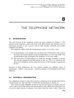
The waveform is shown in Figure 2.1.
The current may then be expressed as
i ¼ðA þkA sin o
s
tÞsin o
c
t ð2:2:5Þ
where
k ¼
B
A
: ð2:2:6Þ
18 AMPLITUDE MODULATED RADIO TRANSMITTER
The factor k is called the depth of modulation and may be expressed as a percentage.
Simplification of Equation (2.2.5) gives
i ¼ A sin o
c

t þ
kA
2
½cos o
c
À o
s
Þt À cosðo
c
þ o
s
Þtð2:2:7Þ
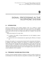
The frequency spectrum is shown in Figure 2.2.
From Equation (2.2.7) it is evident that modulated carrier current has three
distinct frequencies present: the carrier frequency o
c
, the frequency equal to the
difference between the carrier frequency and the modulating signal frequency
Figure 2.1. Amplitude modulated wave: the carrier frequency remains sinusoidal at o
c
while
the envelope varies at frequency o
s
.
Figure 2.2. Frequency spectrum of the AM wave of Figure 2.1. Note that there are three
distinct frequencies present.
2.2 AMPLITUDE MODULATION THEORY 19
(o
c
À o

s
), and the frequency equal to the sum of the carrier frequency and the
modulating signal frequency (o
c
þ o
s
). The difference and sum frequencies are
called the ‘‘lower’’ and ‘‘ upper’’ sidebands, respectively.
To make the situation more realistic, let us assume that the modulating signal is
speech which contains frequencies between o
s1
and o
s2
. Then it follows from
Equation (2.2.7) that the sum and difference terms will yield a band of frequencies
symmetrical about the carrier frequency, as shown in Figure 2.3.
Figure 2.4 shows how two audio signals which would normally interfere with
each other, when transmitted simultaneously through the same medium, can be kept
separate by choosing suitable carrier frequencies in a modulating scheme. This
method of transmitting two or more signals through the same medium simulta-
neously is referred to as frequency-division multiplex and will be discussed in detail
in Chapter 9.
Figure 2.3. Frequency spectrum of the AM wave when the single frequency modulating signal
is replaced by a band of audio frequencies. Note that the information in the signal resides only in
the sidebands.
Figure 2.4. The diagram illustrates how two audio-frequency sources, which would normally
interfere with each other, can be transmitted over the same channel with no interaction.
20 AMPLITUDE MODULATED RADIO TRANSMITTER
2.3 SYSTEM DESIGN
The choice of carrier frequency for a radio transmitter is largely determined by

government regulations and international agreements. It is evident from Figure 2.4
that, in spite of frequency division multiplexing, two stations can interfere with each
other if their carrier frequencies are so close that their sidebands overlap. In theory,
every transmitter must have a unique frequency of operation and sufficient
bandwidth to ensure no interference with others. However, bandwidth is limited
by considerations such as cost and the sophistication of the transmission technique to
be used so that, in practice, two radio transmitters may operate on frequencies which
would normally cause interference so long as they propagate their signals within
specified limits of power and are located (geographically) sufficiently far apart. The
location as well as the power transmitted by each transmitter is monitored and
controlled by the government.
Once the carrier frequency is assigned to a radio station, it is very important that
it maintains that frequency as constant as possible. There are two reasons for this: (1)
if the carrier frequency were allowed to drift then the listeners would have to re-tune
their radios from time to time to keep listening to that station, which would be
unacceptable to most listeners; (2) if a station drifts (in frequency) towards the next
station, their sidebands would overlap and cause interference. The carrier signal is
usually generated by an oscillator, but to meet the required precision of the
frequency it is common practice to use a crystal-controlled oscillator. At the heart
of the crystal-controlled oscillator is a quartz crystal cut and polished to very tight
specifications which maintains the frequency of oscillation to within a few hertz of
its nominal value. The design of such an oscillator can be found in Section 2.4.6.
Figure 2.5 is a block diagram of a typical transmitter.
Figure 2.5. Block diagram showing the components which make up the AM transmitter.
2.3 SYSTEM DESIGN 21
2.3.1 Crystal-Controlled Oscillator
The purpose of the crystal oscillator is to generate the carrier signal. To minimize
interference with other transmitters, this signal must have extremely low levels of
distortion so that the transmitter operates at only one frequency. As discussed earlier,
the frequency must be kept within very tight limits, usually within a few hertz in

10
7
Hz. It is difficult to design an ordinary oscillator to satisfy these conditions, so it
is common practice to use a quartz crystal to enhance the frequency stability and to
reduce the harmonic distortion products.
The quartz crystal undergoes a change in its physical dimensions when a potential
difference is applied across two corresponding faces of the crystal. If the potential
difference is an alternating one, the crystal will vibrate and exhibit the phenomenon
of resonance. For a crystal, the range of frequency over which resonance is possible
is very narrow, hence the frequency stability of the crystal-controlled oscillators is
very high. In general, the larger the physical size of the crystal, the lower the
frequency at which it resonates. Thus a high-frequency crystal is necessarily small,
fragile, and has low reliability. To generate a high-frequency carrier, it is common
practice to use a low-frequency crystal to obtain a signal at a subharmonic of the
required frequency and to use a frequency multiplier to increase the frequency.
Figure 2.5 shows that the crystal-controlled oscillator is followed by a frequency
multiplier.
2.3.2 Frequency Multiplier
The purpose of the frequency multiplier is to accept an incoming signal of frequency
f
c
=n, where n is an integer, and to produce an output at a frequency f
c
. A frequency
multiplier can have a single stage of multiplication or it can have several stages. The
output of the frequency multiplier goes to the carrier input of the amplitude
modulator.
2.3.3 Amplitude Modulator
The amplitude modulator has two inputs, the first being the carrier signal generated
by the crystal oscillator and multiplied by a suitable factor, and the second being the

modulating signal (voice or music) which is represented in Figure 2.5 by the single
frequency f
s
. In reality, the frequencies present in the modulating signal are in the
audio range 20–20,000 Hz. The output from the amplitude modulator consists of the
carrier, the lower and upper sidebands.
2.3.4 Audio Amplifier
The audio amplifier accepts its input from a microphone and supplies the necessary
gain to bring the signal level to that required by the amplitude modulator.
22 AMPLITUDE MODULATED RADIO TRANSMITTER
2.3.5 Radio-Frequency Power Amplifier
The power level at the output of the modulator is usually in the range of watts and
the power required to broadcast the signal effectively is in the range of tens of
kilowatts. The radio-frequency amplifier provides the power gain as well as the
necessary impedance matching to the antenna.
2.3.6 Antenna
The antenna is the circuit element that is responsible for converting the output power
from the transmitter amplifier into an electromagnetic wave suitable for efficient
radiation in free space. Antennae take many different physical forms determined by
the frequency of operation and the radiation pattern desired. For broadcasting
purposes, an antenna that radiates its power uniformly to its listeners is desirable,
whereas in the transmission of signals where security is important (e.g. telephony),
the antenna has to be as directive as possible to reduce the possibility of its reception
by unauthorized persons.
2.4 RADIO TRANSMITTER OSCILLATOR
Perhaps the simplest way to introduce the phenomenon of oscillation is to describe a
common experience of a public address system going unstable and producing an
unpleasantly loud whistle. The system consists of a microphone, an amplifier and a
loudspeaker (or loudspeakers) as shown in Figure 2.6. The amplified sound from the
Figure 2.6. The diagram illustrates how acoustic feedback can cause a public address system

to go unstable, turning the system into an oscillator.
2.4 RADIO TRANSMITTER OSCILLATOR 23
loudspeaker may be reflected from walls and other surfaces and reach the micro-
phone. If the reflected sound is louder than the original then it will in turn produce a
louder output at the loudspeaker which will in turn produce an even louder signal at
the microphone. It is fairly clear that this state of affairs cannot continue indefinitely;
the system reaches a limit and produces the characteristic loud whistle. Immediate
steps have to be taken to ensure that the sound level reaching the microphone is less
than that required to reach the self-sustained value. If, on the other hand, we are
interested in the generation of an oscillation, then the study of the characteristics of
the amplifying element, the conditions under which the feedback takes place, the
frequencies present in the signal and the optimization of the system to achieve
specified performance goals are in order.
The electronic oscillator is a particular example of a more general phenomenon of
systems which exhibit a periodic behavior. A mechanical example is the pendulum
which will perform simple harmonic motion at a frequency determined by its length
and the acceleration constant due to gravity, g, if the energy it loses per cycle is
replaced from an outside source. In the case of the pendulum used in clocks, the
source of energy may be a wound-up spring or a weight whose potential energy is
transferred to the pendulum. The solar system with planets performing cyclical
motion around the sun is another example of an oscillator, although this time there is
no periodic input of energy because the system is virtually lossless.
Three theoretical approaches to oscillator design are presented below. The first is
based on the idea of setting up a ‘‘lossless’’ system by canceling the losses in an LC
circuit due to the presence of (positive) resistance by using a negative resistance. The
second is based on feedback theory. The third is based on the concept of embedding
an active device and the optimization of the power output from the oscillator.
2.4.1 Negative Conductance Oscillator
Consider the circuit shown in Figure 2.7. The externally applied current and the
corresponding voltage are related to each other by

I ¼ G
0
þ G
n
þ sC þ
1
sL

ðV Þð2:4:1Þ
Figure 2.7. The negative conductance oscillator has a negative conductance generating signal
power which is dissipated in the (positive) conductance. The components L and C determine the
frequency of the signal. An alternate statement is that the negative conductance cancels all the
losses in the circuit. It then oscillates losslessly at a frequency determined by L and C.
24 AMPLITUDE MODULATED RADIO TRANSMITTER
where G
0
is the load conductance, G
n
is the negative conductance, I is current, V is
voltage, s is the complex frequency, C is capacitance, and L is inductance. If the
circuit is that of an oscillator, the external excitation current must be zero since an
oscillator does not require an excitation current. Hence
0 ¼ G
0
þ G
n
þ sC þ
1
sL


ðV Þ: ð2:4:2Þ
For a non-trivial solution, V is non-zero, therefore
G
0
þ G
n
þ sC þ
1
sL
¼ 0 ð2:4:3Þ
which gives the quadratic equation
s
2
CL þ sLðG
0
þ G
n
Þþ1 ¼ 0: ð2:4:4Þ
The solution is then
s
1
; s
2
¼À
ðG
0
þ G
n
Þ
2C

Æ
ffiffiffiffiffiffiffiffiffiffiffiffiffiffiffiffiffiffiffiffiffiffiffiffiffiffiffiffiffiffiffiffiffiffi
ðG
0
þ G
n
Þ
2
4C
2
À
1
LC
s
ð2:4:5Þ
when
jG
n
j¼G
0
ð2:4:6Þ
that is, the system is lossless. Equation (2.4.5) becomes
s
1
; s
2
¼
ffiffiffiffiffiffiffiffiffiffiffi
À
1

LC
r
¼ jo
1
ffiffiffiffiffiffiffi
LC
p
ð2:4:7Þ
which is the resonant frequency for the tuned circuit. The circuit will continue to
oscillate at this frequency as if it were in perpetual motion.
A number of devices exhibit negative conductance under appropriate bias
conditions and may be used in the design of practical oscillators of this type.
These include tunnel diodes, pentodes (N-type negative conductance), uni-junction
transistors and silicon-controlled rectifier (S-type).
The voltage–current characteristics of N- and S-type negative conductances are
shown in Figures 2.8(a) and (b), respectively.
2.4 RADIO TRANSMITTER OSCILLATOR 25
2.4.2 Classical Feedback Theory
Consider the system shown in Figure 2.9 where A is the gain of an amplifier and b
represents the transfer function of the feedback path. E
s
is the signal applied to the
input and E
o
is the output of the system [1].
In the derivation that follows, it is necessary to make the following assumptions:
(1) the input impedances of both the amplifier and the feedback network are
infinite and their output impedances are zero,
(2) both A and b are complex quantities.
Figure 2.8. (a) Characteristics of an N-type negative conductance device. The device has a

negative conductance in the region where the slope of the curve is negative. Examples of
practical devices which have such characteristics are the tunnel diode and the tetrode. (b)
Characteristics of an S-type negative conductance device. The device has a negative conduc-
tance in the region where the slope of the curve is negative. Examples of practical devices which
have such characteristics are the four-layer diode and the silicon controlled rectifier.
26 AMPLITUDE MODULATED RADIO TRANSMITTER
The gain of the amplifier alone is
A ¼
E
o
E
g
: ð2:4:8Þ
Application of Kirchhoff’s Voltage Law (KVL) at the input gives
E
g
¼ E
s
þ bE
o
: ð2:4:9Þ
Substituting Equation (2.4.8) into Equation (2.4.9) gives
E
o
¼ AðE
s
þ bE
o
Þð2:4:10Þ
from which we obtain

E
o
E
s
¼
A
1 À bA
: ð2:4:11Þ
Since the E
s
and E
o
are the input and output, respectively, of the system as a whole,
we can define this as A
0
where
A
0
¼
E
o
E
s
¼
A
ð1 À bAÞ
: ð2:4:12Þ
Three separate conditions must be considered that depend on the value of the
denominator of Equation (2.4.12)
(1) Positive feedback. If the modulus of ð1 À bAÞ is less than unity, then the gain

of the system A
0
is greater then the gain of the amplifier A and therefore the
effect of the feedback is said to be positive.
(2) Negative feedback. If the modulus of ð1 À bAÞ > 1, then A
0
< A.
Figure 2.9. Classical feedback system with gain A and feedback factor b.
2.4 RADIO TRANSMITTER OSCILLATOR 27
(3) Oscillation. If the modulus of ð1 À bAÞ¼0 then the gain A
0
is infinite
because with no input ðE
s
¼ 0Þ there is still an output. In fact the system is
supplying its own input and
bA ¼ 1: ð2:4:13Þ
It must be noted that the waveform of the signal need not be sinusoidal and in fact it
can take any form so long as the waveform of the signal that is fed back, bE
o
,is
identical to the signal E
o
. However, the object of this exercise is to generate a carrier
for a telecommunication system and therefore only sinusoidal signals are acceptable
– any other waveform will generate other carriers (harmonics of the fundamental)
and cause interference with transmissions of other stations.
2.4.3 Sinusoidal Oscillators
Since both A and b are complex quantities, condition (3) implies
jbAj¼1: ð2:4:14Þ

Stated in words, the magnitude of the loop gain must equal unity, and
ffbA ¼ 0; 2p; 4p; etc. ð2:4:15Þ
Again, in words, the loop-gain phase shift must be zero or an integral multiple of 2p
radians. The condition given in Equation (2.4.13), which implies Equations (2.4.14)
and (2.4.15), is known as the Barkhausen Criterion.
These two conditions must exist simultaneously for sinusoidal oscillation to
occur.
2.4.4 General Form of the Oscillator
An oscillator circuit shown in Figure 2.10 [2] and an equivalent circuit is as shown in
Figure 2.11, where the amplifying element is replaced by a voltage-controlled
voltage source in series with a resistance R
o
to simulate the output resistance of the
element. The amplifying element may be a tube, a transistor or an operational
amplifier.
The load seen by the amplifier is
Z
L
¼
Z
2
ðZ
1
þ Z
3
Þ
ðZ
1
þ Z
2

þ Z
3
Þ
: ð2:4:16Þ
28 AMPLITUDE MODULATED RADIO TRANSMITTER
The amplifier gain without feedback is
A ¼
V
o
V
32
¼À
A
v
Z
L
ðR
o
þ Z
L
Þ
ð2:4:17Þ
and the feedback constant is
b ¼
Z
1
ðZ
1
þ Z
3

Þ
: ð2:4:18Þ
The loop gain is
bA ¼À
A
v
Z
1
Z
L
ðR
o
þ Z
L
ÞðZ
1
þ Z
3
Þ
: ð2:4:19Þ
Figure 2.10. Circuit diagram for a more generalized form of the oscillator.
Figure 2.11. The equivalent circuit of the generalized form of the oscillator. R
o
represents the
output resistance of the amplifier.
2.4 RADIO TRANSMITTER OSCILLATOR 29
Substituting for Z
L
as defined in Equation (2.4.16), Equation (2.4.19) becomes
bA ¼À

A
v
Z
1
Z
2
½R
o
ðZ
1
þ Z
2
þ Z
3
ÞþZ
2
ðZ
1
þ Z
3
Þ
: ð2:4:20Þ
For simplicity, we may assume that the impedances are lossless; hence
Z
1
¼ jX
1
; Z
2
¼ jX

2
and Z
3
¼ jX
3
ð2:4:21Þ
Then Equation (2.4.20) becomes
bA ¼À
A
v
X
1
X
2
½jR
o
ðX
1
þ X
2
þ X
3
ÞÀX
2
ðX
1
þ X
3
Þ
: ð2:4:22Þ

Recall that for oscillation to occur
1 À bA ¼ 0: ð2:4:23Þ
This means that bA must be real and hence,
X
1
þ X
2
þ X
3
¼ 0 ð2:4:24Þ
that is,
X
2
¼ÀðX
1
þ X
3
Þ: ð2:4:25Þ
The expression for the loop gain becomes
bA ¼ÀA
v
X
1
X
2
: ð2:4:26Þ
Since bA ¼ 1, it follows that X
1
and X
2

must have opposite signs; that is, if one of
them is inductive, the other must be capacitive and X
3
can be capacitive or inductive,
depending on the sign of (X
1
þ X
2
). The two possibilities are shown in Figures 2.12
and 2.13, respectively.
The circuit shown in Figure 2.12 is better known as a Colpitts oscillator. The
circuit is redrawn in Figure 2.12(b) to emphasize the symmetrical structure of the
circuit.
The circuit shown in Figure 2.13 is better known as a Hartley oscillator.
From the point of view of the structure of the circuits, it can be seen that they are
the same. It should be noted that the operational amplifier can be replaced by a tube
or a transistor.
30 AMPLITUDE MODULATED RADIO TRANSMITTER
2.4.5 Oscillator Design for Maximum Power Output
A major flaw in the two previous designs is that they do not anticipate the necessity
for the oscillator to supply power to a load. The theory of the design for maximum
power output from an oscillator [3] is based on the characterization of the amplifying
element (‘‘ active device’’) as a two-port. A discussion of two-ports is beyond the
scope of this book but may be found in any standard text on circuit theory.
A two-port can be described in terms of its terminal voltages and currents by four
parameters: impedances, admittances, voltage ratios, and current ratios under
constraints of open or short-circuit. Without limiting the generality, assume that
the active device has been characterized in terms of the short-circuit admittance
Figure 2.12. (a) The generalized form of the oscillator with two of the impedances replaced by
capacitors and the third by an inductor to form a Colpitts oscillator. (b) The diagram in (a) has

been redrawn to emphasize the symmetry of the circuit.
Figure 2.13. (a) The generalized form of the oscillator with two of the impedances replaced by
inductors and the third by a capacitor to form a Hartley oscillator. (b) The diagram in (a) has been
redrawn to emphasize the symmetry of the circuit.
2.4 RADIO TRANSMITTER OSCILLATOR 31
parameters, or Y parameters, for short. Figure 2.14 shows the two-port and its
terminal voltages and currents, which are assumed to be sinusoidal.
The Y parameters are functions of frequency and bias conditions, and in general,
complex so that
Y
11
¼ g
11
þ jb
11
: ð2:4:27Þ
The total power entering the two-port is
P ¼ V
Ã
1
I
1
þ V
Ã
2
I
2
: ð2:4:28Þ
The Y parameters and the terminal voltages and currents are related by
I

1
¼ Y
11
V
1
þ Y
12
V
2
ð2:4:29Þ
and
I
2
¼ Y
21
V
1
þ Y
22
V
2
: ð2:4:30Þ
Substituting for I
1
and I
2
in Equation (2.4.28) gives
P ¼ Y
11
jV

1
j
2
þ Y
22
jV
2
j
2
þ Y
12
V
Ã
1
V
2
þ Y
21
V
1
V
Ã
2
: ð2:4:31Þ
The ratio of the output voltage, V
2
, to the input voltage, V
1
, can be defined as
V

2
V
1
¼ A ¼ A
R
þ jA
I
: ð2:4:32Þ
The real power entering the two-port is
P
R
¼jV
1
j
2
½g
11
þ g
22
ðA
2
R
þ A
2
I
Þþðg
12
þ g
21
ÞA

R
Àðb
12
þ b
21
ÞA
I
: ð2:4:33Þ
Figure 2.14. A two-port representation of an active device to be used in the design of an
oscillator. Short-circuit admittance (Y) parameters are used in the design for convenience. Other
parameters could be used in the description.
32 AMPLITUDE MODULATED RADIO TRANSMITTER
This can be rearranged as follows:
P
R
g
22
jV
1
j
2
¼ A
R
þ
ðg
21
þ g
12
Þ
2g

22

2
þ A
I
þ
ðb
21
À b
21
Þ
2g
22

2
þ
4g
11
g
22
Àðg
21
þ g
12
Þ
2
Àðb
21
À b
12

Þ
2
4g
2
22
: ð2:4:34Þ
This equation is of the form:
z ¼ðx ÀaÞ
2
þðy ÀbÞ
2
þ c ð2:4:35Þ
and therefore it is that of a paraboloid in space with axes P
R
ðg
22
=V
1
=
2
Þ, A
R
and A
I
as
shown in Figure 2.15.
It was assumed that real, positive power was supplied and dissipated in the two-
port; therefore, it follows that negative values of power, as shown in Figure 2.15,
must represent power generated by the two-port and dissipated in the surrounding or
embedding circuit; that is, above the A plane, real power is supplied to the two-port,

and below it the device supplies real power to the embedding circuit. Because the
object of the exercise is to generate and supply real power to an external circuit, the
most interesting part of Figure 2.15 is the part below the A plane. It is clear that
movement towards the apex of the paraboloid represents increasing levels of power
supplied by the ‘‘ active’’ two-port and that the maximum power supplied occurs at
the apex. We shall return to this remark when we consider the optimization of the
power output.
The most general embedding circuit for the two-port is as shown in Figure 2.16
with each branch made up of a conductance in parallel with a susceptance. The
susceptances can be considered as the tuned circuit which will determine the
Figure 2.15. Three-dimensional representation of the output power of the oscillator as a
function of the complex parameter A.
2.4 RADIO TRANSMITTER OSCILLATOR 33
frequency of oscillation and the conductances as the destination of the power
generated by the active two-port.
The embedding network can also be described in terms of a two-port as follows:
I
0
1
¼ðY
2
þ Y
3
ÞV
1
À Y
3
V
2
ð2:4:36Þ

I
0
2
¼ÀY
3
V
1
þðY
1
þ Y
3
ÞV
2
: ð2:4:37Þ
When the active device and the embedding are connected as shown in Figure 2.17,
the composite circuit can be described by the two-port equations which are
[Equations (2.4.29) þ (2.4.36) and Equations (2.4.30) þ (2.4.37)]:
I
1
þ I
0
1
¼ðY
11
þ Y
2
þ Y
3
ÞV
1

þðY
12
À Y
3
ÞV
2
ð2:4:38Þ
I
2
þ I
0
2
¼ðY
21
À Y
3
ÞV
1
þðY
1
þ Y
3
þ Y
22
ÞV
2
: ð2:4:39Þ
Figure 2.16. The general passive embedding circuit for a two-port.
Figure 2.17. The active two-port is shown with the passive embedding connected.
34 AMPLITUDE MODULATED RADIO TRANSMITTER

For an oscillator, no external signal current is supplied at port 1 and therefore
I
1
þ I
0
1
¼ 0. Similarly I
2
þ I
0
2
¼ 0. From Equation (2.4.32) we have
V
2
¼ V
1
ðA
R
þ jA
I
Þð2:4:40Þ
From Equation (2.4.38) we have
V
1
½Y
11
þ Y
2
þ Y
3

þðA
R
þ jA
I
ÞðY
12
À Y
3
Þ ¼ 0 ð2:4:41Þ
and from Equation (2.4.39) we have
V
1
½Y
21
À Y
3
þðA
R
þ jA
I
ÞðY
1
þ Y
3
þ Y
22
Þ ¼ 0: ð2:4:42Þ
For non-trivial values of V
1
, real and imaginary values of Equations (2.4.41) and

(2.4.42) are separately equal to zero; that is,
g
11
þ G
2
þ G
3
þ A
R
ðg
12
À G
3
ÞÀA
I
ðb
12
À B
3
Þ¼0 ð2:4:43Þ
b
11
þ B
2
þ B
3
þ A
R
ðb
12

À B
3
ÞþA
I
ðg
12
À G
3
Þ¼0 ð2:4:44Þ
g
21
À G
3
þ A
R
ðG
1
þ G
3
þ g
22
ÞÀA
I
ðB
1
þ B
3
þ b
22
Þ¼0 ð2:4:45Þ

and
b
21
À B
3
þ A
R
ðB
1
þ B
3
þ b
22
ÞþA
I
ðG
1
þ G
3
þ g
22
Þ¼0: ð2:4:46Þ
Equations (2.4.43) to (2.4.46) can be written in the form of a matrix as follows:
A
R
0 ðA
R
À 1ÞÀA
I
0 ÀA

I
A
I
0 A
I
A
R
0 ðA
R
À 1Þ
01ð1 ÀA
R
Þ 00 A
I
00 ÀA
I
01ð1 ÀA
R
Þ
2
6
6
4
3
7
7
5
G
1
G

2
G
3
B
1
B
2
B
3
2
6
6
6
6
6
6
4
3
7
7
7
7
7
7
5
¼
Àg
21
ÀReðAy
22

Þ
Àb
21
ÀImðAy
22
Þ
Àg
11
ÀReðAy
12
Þ
Àb
11
ÀImðAy
12
Þ
2
6
6
4
3
7
7
5
ð2:4:47Þ
All the terms in the matrix are known except G
1
, G
2
, G

3
, B
1
, B
2
and B
3
; that is, there
are six unknowns but only four equations so a unique solution cannot be found
unless arbitrary values are chosen for at least two of the unknowns. Fortunately, an
oscillator normally has only one conductive load and therefore two of the three
conductances can be set to zero. The matrix equation can then be solved for one
conductance and three susceptances.
2.4.6 Crystal-Controlled Oscillator
The oscillator used in a transmitter has to have a very tight tolerance on the stability
of its frequency. This is necessary if interference between radio stations is to be
2.4 RADIO TRANSMITTER OSCILLATOR 35
avoided. The drift of the frequency of an ordinary LC oscillator, for example, makes
it unsuitable for this purpose. Greater frequency stability can be achieved by using a
crystal as a part of the oscillator circuit [4]. In Section 2.3.1, the behavior of the
crystal when it is excited by an ac signal was discussed. It is evident that, since the
crystal reacts to electrical excitation, it must be possible to devise an electrical circuit
made up of inductors, resistors and capacitors whose frequency characteristics are
approximately those of the crystal. Such a circuit is shown in Figure 2.18. The
approximate circuit is reasonably accurate at frequencies close to the resonant
frequency. Over a larger frequency range a more complicated equivalent circuit has
to be used.
Typical values of the components of the equivalent circuit are C ¼ 0:0154 pF,
R ¼ 8 O, L ¼ 0:0165 H, C
o

¼ 4:55 pF. The capacitance C
o
is due largely to the
electrodes which are attached to the crystal. The crystal will therefore resonate in the
series mode at a frequency o
s
where
o
2
s
¼
1
LC
ð2:4:48Þ
which gives f
s
¼ 9:984 Â 10
6
Hz. It will resonate in the parallel mode at an angular
frequency given approximately by
o
2
p
¼
1
L
CC
o
ðC þ C
o

Þ

ð2:4:49Þ
which gives a resonant frequency, f
p
¼ 10:001 Â10
6
Hz – a change of less than
0.2%. The corresponding quality factor of the crystal is then Q
o
¼ 130;000.
Figure 2.18. (a) The equivalent circuit of the crystal and its package. (b) The electrical symbol
for the crystal.
36 AMPLITUDE MODULATED RADIO TRANSMITTER
Figure 2.19 shows the reactance of the crystal plotted against frequency. It should
be noted that the reactance of the crystal is inductive over a narrow band of
frequency and also that both reactance and frequency are not to scale.
Figure 2.20 shows a typical crystal-controlled oscillator. The crystal is substituted
for one of the inductors in what would otherwise be classified as a Hartley oscillator.
This type of crystal-controlled oscillator is called a Pierce oscillator. Similarly, the
crystal-controlled oscillator corresponding to the Colpitts variety is called a Miller
oscillator. In the circuit shown in Figure 2.20, the active element is a field-effect
transistor whose gate-to-drain capacitance plus stray capacitance constitute C
3
.
The very high Q
o
of the crystal ensures that the oscillator has an extremely
limited range of frequencies in which it can continue to oscillate. Various other
measures may be taken to improve the frequency stability, such as placing the crystal

in a temperature-controlled environment and the Q factor can be enhanced by
evacuating the glass envelope which protects it.
High precision oscillators are invariably connected to their load through a buffer
amplifier. This ensures that variations in the load do not affect the operation of the
oscillator.
2.5 FREQUENCY MULTIPLIER
The purpose of the frequency multiplier is to raise the frequency generated by the
crystal-controlled oscillator to the value required for the transmitter carrier. As
explained earlier, it is not possible to obtain physically robust crystals at high
Figure 2.19. The reactance characteristics of the crystal. Note that this is not to scale.
2.5 FREQUENCY MULTIPLIER 37
frequency since their physical size gets smaller as the frequency of oscillation gets
higher. The standard technique is therefore to use a crystal to generate a signal at a
frequency which is a subharmonic of the required carrier frequency and then to raise
the frequency up to the required value using a cascade of frequency multipliers.
A useful analog of a frequency multiplier is a child’s swing. With a child on the
swing, the adult must give it a push to get the swing into operation. Subsequent to
that, further supplies of energy must take place at a frequency determined by the
length of the swing and the gravitational constant of acceleration, g. It is also
necessary to supply the energy at a point in time when it enhances the swinging
action rather than oppose it; on average, the adult will have to supply energy equal to
that lost during the cycle to maintain a constant amplitude. If the energy supplied per
cycle is less than the energy lost, the amplitude of the swing will decrease to a
smaller value so as to restore the energy balance. If the energy supplied per cycle
is greater than that lost per cycle, the amplitude will grow to a new steady-state
value. The motion of the child will be very nearly a simple harmonic one if the total
energy stored in the system is large compared to the energy supplied by the adult,
that is, the system Q has to be large if the child is to execute a near-sinusoidal
motion. The most important point of this analog is that the energy does not have to
be supplied at the same frequency as the swing: it can be supplied at a subharmonic

frequency, that is, the push can be given every other cycle of the swing or every third
cycle or higher so long as enough energy is supplied to maintain the energy balance.
When the push occurs every other cycle, it is clear that the output of the system is at
twice the frequency of the input – this is a frequency multiplier with a multiplication
Figure 2.20. (a) A Hartley oscillator with one of the inductors replaced by a crystal. This circuit
is called a Pierce oscillator. The field-effect transistor may be replaced by any other suitable
active device. (b) The equivalent circuit of the Pierce oscillator demonstrating its symmetrical
structure.
38 AMPLITUDE MODULATED RADIO TRANSMITTER
factor of two. When the energy is supplied every third cycle, the multiplication
factor of three is obtained, and so on. Evidently, there is a limit on how high the
multiplication factor can be and it is determined by the amount of variation in the
amplitude of the swing which can be tolerated. Table 2.1 shows a comparison of the
swing and the frequency multiplier.
Figure 2.21 shows a typical frequency multiplier. Energy is fed into it by applying
a suitable positive pulse to the base of the transistor. This causes the transistor to
conduct momentarily, that is, current flows from the direct current (dc) power supply
through the inductor and a finite amount of energy is stored in the inductor. The
current flow is shut off when the input pulse ends and the transistor is essentially an
open-circuit. The energy stored in the magnetic field of the inductor is transformed
into energy stored in the electric field of the capacitor. The transformation of energy
from one form to another and back again would continue indefinitely in a sinusoidal
form if the system were lossless and this would take place at a frequency determined
by the values of the inductance and capacitance. The resistance R
L
represents the
losses in the system – the amplitude of the sinusoid will decay with time. The
steady-state amplitude of the voltage or current will be determined by the equaliza-
TABLE 2.1 Swing Analogy for a Frequency Multiplier
Swing, Including Child Frequency Multiplier

Adult (timing) Input signal source
Adult (energy transferred to child) DC power supply
Length of swing, l, and gravitational constant, g Inductance, L, and capacitance, C
Air resistance and bearing friction Energy loss in R
Frequency f ¼
1
2p
ffiffiffi
1
g
r
Frequency f ¼
1
2p
ffiffiffiffiffiffiffi
LC
p
Amplitude of swing Amplitude of voltage or current in tank circuit
Figure 2.21. A class-C amplifier to be used, with minor modifications, as a frequency
multiplier.
2.5 FREQUENCY MULTIPLIER 39
tion of the energy input and the energy output (loss). Subsequent to the initial input
pulse, all input pulses must be timed to enhance rather than oppose the stored energy
of the system. It is, of course, not necessary to have an input pulse for every cycle of
the output; the input pulse can be supplied once for every two, three or greater
number of cycles. When the input frequency is the same as the output, the frequency
multiplier (multiplication factor ¼1) is simply a class-C amplifier. Since a class-C
amplifier represents the simplest frequency multiplier, the design of a class-C
amplifier will be discussed next.
2.5.1 Class-C Amplifier

In a class-C amplifier, the current in the active device flows for a period much less
than p radians of the output waveform. The active device current waveform is
therefore highly non-sinusoidal. In a class-A or -B amplifier this would give a
correspondingly non-sinusoidal output. However, in the class-C amplifier the
collector load consists of a parallel LC circuit which is tuned to the frequency of
the input signal. The tuned circuit (sometimes referred to as a tank circuit) presents a
very high impedance at the resonant frequency to the collector of the transistor and
hence a high gain is obtained at this frequency. Other frequencies, such as harmonics
of the input frequency, are attenuated. Therefore, the output is very nearly sinusoidal.
In a practical class-C amplifier, the base of the transistor is held at a voltage such
that the transistor is in the off state. The input signal brings the transistor into
conduction at its positive peaks and causes enough current to flow in the inductor to
store energy equal to that dissipated in the load resistor R
L
and at other sites in the
circuit. When the input signal drops below the threshold of the transistor, it switches
off and the LC tank oscillates freely with a sinusoidal waveform at the resonant
frequency of the tank circuit. Because of the dissipation in the circuit, the waveform
is actually an exponentially damped sinusoid as shown in Figure 2.22.
The collector voltage, the base voltage and collector current waveforms are
shown in Figure 2.23. Note that the quiescent value of the collector voltage
waveform is V
cc
and that its maximum amplitude is 2V
cc
.
The conversion efficiency of the amplifier is given by:
Z ¼ (ac power output)=(dc power input):
A class-C amplifier can have a relatively high conversion efficiency, usually about
85%, because the dc current flows for a very short part of the cycle and this happens

when the collector voltage is at its lowest value. Thus the power lost in the transistor
is minimal.
2.5.2 Converting the Class-C Amplifier into a Frequency Multiplier
To convert a class-C amplifier into a frequency multiplier with a multiplication factor
of 2, the L and C of the tank circuit are chosen to resonate at 2o
o
when the input
signal frequency is o
o
. Successful operation of the system demands that the Q factor
40 AMPLITUDE MODULATED RADIO TRANSMITTER
Figure 2.22. The output waveform of a class-C amplifier after a single pulse excitation. Note
the sinusoidal waveform and the exponential decay of the envelope.
Figure 2.23. The collector voltage (v
c
), base voltage (v
be
) and collector current (i
c
) of the class-
C amplifier. Note that the base voltage need not be sinusoidal for the collector voltage to be
sinusoidal.
2.5 FREQUENCY MULTIPLIER 41