Thông tin thiết kế mạch P3 docx

3
THE AMPLITUDE MODULATED
RADIO RECEIVER
3.1 INTRODUCTION
The electromagnetic disturbance created by the transmitter is propagated by the
transmitter antenna and travels at the speed of light as described in Chapter 2. It is
evident that, if the electromagnetic wave encounters a conductor, a current will be
induced in the conductor. How much current is induced will depend on the strength
of the electromagnetic field, the size and shape of the conductor and its orientation to
the direction of propagation of the wave. The conductor will then capture some of
the power present in the wave and hence it will be acting as a receiver antenna.
However, other electromagnetic waves emanating from all other radio transmitters
will also induce some current in the antenna. The two basic functions of the radio
receiver are:
(1) to separate the signal induced in the antenna by the transmission which we
wish to receive from all the other signals present,
(2) to recover the ‘‘message’’ signal which was used to modulate the transmitter
carrier.
3.2 THE BASIC RECEIVER: SYSTEM DESIGN
In order to separate the required signal from all the other signals captured by the
antenna, we use a bandpass filter centered on the carrier frequency with sufficient
bandwidth to accommodate the upper and lower sidebands but with a sufficiently
high Q factor so that all other carriers and their sidebands are attenuated to a level
where they will not cause interference. This is most easily achieved by using an LC
tuned circuit whose resonant frequency is that of the carrier.
79
Telecommunication Circuit Design, Second Edition. Patrick D. van der Puije
Copyright # 2002 John Wiley & Sons, Inc.
ISBNs: 0-471-41542-1 (Hardback); 0-471-22153-8 (Electronic)
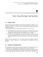
Figure 3.1. (a) The envelope detector circuit. The diode ‘‘half-wave’’ rectifies the AM wave and
the RC time-constant ‘‘follows’’ the envelope with a slight ripple. (b) The input signal to the

envelope detector. (c) The output signal of the envelope detector. Note that (1) when the voltage
is rising the ripple is larger than when the voltage is falling. A longer time constant will help
reduce the ripple; however, it will also increase the likelihood that the output voltage will not
follow the envelope when the voltage is falling causing ‘diagonal clipping’. (2) In practice, the
carrier frequency is much higher than the modulating frequency, hence the ripple is much smaller
than shown.
80 THE AMPLITUDE MODULATED RADIO RECEIVER
To recover the ‘‘message’’ we require a circuit which will follow the envelope of
the amplitude of the carrier. Such a circuit is called an envelope detector and it
consists of a diode and a parallel RC circuit as shown in Figure 3.1(a).
The input signal to the circuit is most appropriately represented by an ideal
current source connected to the primary of the transformer. This ideal current source
represents all the currents induced in the antenna by all the radio stations broad-
casting signals in free space. The signal is coupled to the parallel-tuned LC circuit
which selectively enhances the amplitude of the signal whose carrier frequency is the
same as the resonant frequency of the LC circuit. In Figure 3.1(b), only the enhanced
modulated signal is shown at the input of the envelope detector. Because the diode
conducts only when the anode has a positive potential compared to the cathode, only
the positive half of the signal appears across the output resistor. Because the
capacitor is connected in parallel with the resistor, when the diode conducts the
capacitor must charge up to the peak value of the voltage. When the input voltage is
less than the voltage across the capacitor, the conduction is cut off and the capacitor
starts to discharge through the resistor with the voltage falling off exponentially.
With the proper choice of time-constant RC, the output voltage waveform will have
the form shown in Figure 3.1(c). This waveform is essentially the envelope of the
carrier signal with a ripple at a frequency equal to the carrier frequency. A low-pass
filter can be used to remove the ripple.
The circuit shown in Figure 3.1(a) has been used with success as a practical
receiver with the resistor R replaced by a high impedance headphone. Needless to
say, such a simple circuit has its limitations. The power in the circuit is supplied

entirely by the transmitter and naturally it is at a very low level, especially as the
distance between the transmitter and the receiver increases. Secondly, the ability of
the LC tuned circuit to suppress the signals propagated by all the other transmitters is
limited and therefore such a receiver will be subject to interference from other
stations. These limitations can be overcome by using the superheterodyne config-
uration described below.
Figure 3.1. (continued )
3.2 THE BASIC RECEIVER: SYSTEM DESIGN 81
3.3 THE SUPERHETERODYNE RECEIVER: SYSTEM DESIGN
The superheterodyne receiver takes the incoming radio-frequency signal whose
frequency varies from station to station and transforms it to a fixed frequency called
the intermediate frequency (IF). It is then easier to do the necessary filtering to
eliminate interference and, at the same time, to provide some power gain or
amplification to the desired signal.
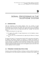
A normal AM superheterodyne receiver block diagram is shown in Figure 3.2.
The antenna has induced in it currents from all the transmitters whose electro-
magnetic propagation reach it. The first step is to use an LC tuned radio-frequency
amplifier to enhance the desired carrier and its sidebands. The radio-frequency
amplifier is tuneable over the frequency for which the receiver is designed by
varying the capacitor in the tuned circuit. This capacitor is mechanically coupled or
‘‘ganged’’ to another capacitor which forms part of the local oscillator circuit. The
local oscillator frequency and the frequency to which the radio-frequency amplifier
is tuned are chosen in such a way that, as the value of the ganged capacitors change,
they maintain a fixed frequency difference between them. The outputs from the local
oscillator and the radio-frequency amplifier are used to drive the frequency changer
or mixer. The frequency changer essentially multiplies the two inputs and produces a
signal that contains the sum and difference of the input frequencies. Because of the
fixed difference between the incoming radio-frequency and the local oscillator
frequency, the difference frequency remains constant as the value of the ganged
capacitor is changed. The output of the frequency changer is then fed into the

intermediate-frequency amplifier. The intermediate-frequency amplifier is designed
to select the difference frequency plus its sidebands and to attenuate all other
frequencies present. Since the difference frequency is fixed (for domestic AM radios
the intermediate frequency is 445 kHz) the filters required are relatively easy to
Figure 3.2. The block diagram of the superheterodyne receiver. The capacitor which tunes the
radio-frequency amplifier is mechanically ganged to the capacitor which determines the
frequency of the local oscillator. In the normal AM receiver, the oscillator frequency is always
455 kHz above the resonant frequency of the radio-frequency amplifier throughout the range of
tuning.
82 THE AMPLITUDE MODULATED RADIO RECEIVER
design with sharp cut-off characteristics. The output of the intermediate-frequency
amplifier which then goes to the envelope detector consists of the intermediate
frequency and its two sidebands. The envelope detector removes the intermediate
frequency, leaving the audio-frequency signal which is then amplified by the audio-
frequency amplifier to a level capable of driving the loudspeaker. It is clear that there
will be a very large difference between the signal from a powerful local radio station
and a weak distant station. To help reduce the difference an automatic gain control
(AGC) is used to adjust the signal reaching the envelope detector to stay within
predetermined values.
The most interesting signal processing step in the system takes place in the
frequency changer or frequency mixer or simply the mixer [1]. There are two basic
types of mixers: the analog multiplier and the switching types. The analog multiplier
frequency changer simply multiplies the radio-frequency signal and the local
oscillator so that when the modulated carrier current is
i
m
ðtÞ¼Að1 þ k sin o
S
tÞ sin o
C

t ð3:3:1Þ
and the local oscillator signal is
i
o
ðtÞ¼B sin o
L
t ð3:3:2Þ
the output of the mixer is
iðtÞ¼Að1 þ k sin o
S
tÞ sin o
C
t  B sin o
L
t ð3:3:3Þ
iðtÞ¼
1
2
ABð1 þ k sin o
S
tÞ½cosðo
L
À o
C
Þt À cosðo
L
þ o
C
Þtð3:3:4Þ
iðtÞ¼

1
2
AB½cosðo
L
À o
C
Þt À cosðo
L
þ o
C
Þt þ k sin o
S
t cosðo
L
À o
C
Þt
À k sin o
S
t cosðo
L
þ o
C
Þtð3:3:5Þ
iðtÞ¼
1
2
ABfcosðo
L
À o

C
Þt À cosðo
L
þ o
C
Þt
þ
1
2
k½sinðo
L
À o
C
À o
S
Þt þ sinðo
L
À o
C
þ o
S
Þt
À
1
2
k½sinðo
L
þ o
C
À o

S
Þt þ sinðo
L
þ o
C
þ o
S
Þtg: ð3:3:6Þ
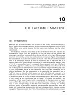
The spectrum of Equation (3.3.6) is shown in Figure 3.3. It should be noted that this
has been simplified for clarity. The product formation in Equation (3.3.3) is not a
precise process and tends to create a large number of frequencies due to sub- and
higher harmonics present in both the radio-frequency and local oscillator signals.
The radio-frequency and local oscillator signals are usually present in the output as
well. It is important to keep all the unwanted signals outside the frequency band of
the intermediate frequency and, failing that, to reduce their amplitude to a very low
value.
It can be seen that the mixing operation gives two additional carriers and their
sidebands at frequencies corresponding to the sum (o
L
þ o
C
) and difference
(o
L
À o
C
) of the local oscillator and carrier frequencies. The required signal at
3.3 THE SUPERHETERODYNE RECEIVER: SYSTEM DESIGN 83
the difference frequency (intermediate frequency) can now be filtered out by the
intermediate-frequency stage of the receiver. It should be noted that the mixing

operation does not affect the sidebands. To clarify the changes in frequency that take
place as the signal proceeds through the system, the AM broadcast band (600 kHz–
1600 kHz) is used as an example in Table 3.1.
The frequency changer or mixer presents two immediate problems: the choice of
the local oscillator frequency and the design strategy of the mixer itself.
(1) It can be seen from Table 3.1 that the local oscillator frequency has been
chosen to be higher than the incoming radio-frequency signal. There is a very
good reason for this. The ratio of the maximum to the minimum capacitance
Figure 3.3. A simplified spectrum of the output from a frequency changer which uses a
nonlinear device.
TABLE 3.1
Radio frequency (kHz)
Low-frequency end High-frequency end
Incoming signal, f
c
Æ f
s
600 Æ 5 1600 Æ 5
Local oscillator, f
L
600 þ 455 ¼ 1055 1600 þ 455 ¼ 2055
Intermediate frequency, f
k
455 455
Image frequency
a
, f
im
1055 þ 455 ¼ 1510 2055 þ 455 ¼ 2510
Output, intermediate-frequency amplifier, f

k
Æ f
s
455 Æ 5 455 Æ 5
Envelope detector, f
s
0–5 0–5
a
The image frequency is the frequency of the unwanted signal which, when combined with the local oscillator
frequency, will give the intermediate frequency. Normally the radio-frequency amplifier should suppress the
image frequency but this may be difficult if the signal from the desired station is very weak and the image
signal is very strong.
84 THE AMPLITUDE MODULATED RADIO RECEIVER
required to tune the local oscillator across the broadcast band is 3.79
when a higher local oscillator frequency is chosen. If the lower local
oscillator frequency had been chosen, the ratio would have been 62.4.
Such a variable capacitor would be difficult to manufacture with reasonable
tolerance.
(2) The mixing operation was treated earlier as an analog multiplication.
However, the realization of a precise analog multiplier is a non-trivial
problem. A crude analog multiplication can be achieved by using a device
whose voltage–current characteristics are non-linear. An ordinary p–n junc-
tion diode can be used to perform the task. The derivation of the output signal
is similar to that given in Section 2.6.1 and will therefore not be repeated
here.
The switching type of mixer uses a device such as a diode or transistor carrying a
current proportional to the radio-frequency signal and switches it from one state to
another at the local oscillator frequency.
3.4 COMPONENTS OF THE SUPERHETERODYNE RECEIVER
3.4.1 Receiver Antenna

The AM receiver antenna can take many different forms such as the ferrite bar found
in most portable receivers, the whip antenna found on automobiles, and the outdoor
wire type consisting of several metres of wire strung between two towers. In general,
the longer and higher off the ground the antenna is, the more likely it is that it will
have a strong signal induced in it by the electromagnetic signals propagated by the
transmitters. The level of signal induced in the antenna may vary from a few
microvolts to a few volts, depending on the proximity of the transmitter, its radiated
power output, the size of the receiver antenna, and its orientation to the transmitter.
Because of the tremendous variation in the input signal a fixed gain amplifier will
very often either not provide enough signal to the frequency changer or will overload
it and consequently generate a large number of undesirable frequencies. To ensure a
reasonable reception of the largest number of broadcasting stations, the gain of the
amplifier is controlled automatically by the incoming signal – the weaker the signal,
the higher the gain of the radio-frequency amplifier.
The antenna signal is coupled by a radio-frequency transformer to the input of the
radio-frequency amplifier. The transformer is made up of two coils, each containing
several turns of wire wound on a coil former which may or may not have a ferrite
core. The major consideration in the design of the transformer is that the primary
inductance be sufficiently high to ensure that signals at the lowest frequency of
interest are not unduly attenuated. Since the signal frequency can vary from 600 to
1600 kHz, the transformer is not tuned.
3.4 COMPONENTS OF THE SUPERHETERODYNE RECEIVER 85
3.4.2 Low-Power Radio-Frequency Amplifier
Since the input voltage of the amplifier is of the order of microvolts and the signal to
be delivered to the demodulator is usually in volts, the amplifier must have a high
gain. A multi-stage amplifier has to be used to realize the necessary gain. Some of
the stages of gain can be placed before the frequency changer, in which case they are
referred to as the radio-frequency amplifier stage, or after the frequency changer, in
which case they are called the intermediate-frequency amplifier stage. It is usual to
design the radio-frequency amplifier stage for a modest gain and the intermediate-

frequency stage for high gain. Both the radio-frequency and intermediate-frequency
amplifiers are narrow-band amplifiers. This is evident from calculating the Q factor
for the two types of amplifiers. Considering that the normal bandwidth of the AM
radio is 0–5 kHz, both radio-frequency and intermediate-frequency amplifiers have
to have a bandwidth of at least 10 kHz.
The Q factor of the radio-frequency amplifier at the low end of the broadcast band
(600 kHz) is 60 and at the high end (1600 kHz) is 160. The Q factor of the
intermediate-frequency amplifier (centre frequency 455 kHz) is 45. However, opera-
tion of the radio-frequency amplifier with such a high Q factor will cause serious
tracking problems with the local oscillator and will also lead to excessive attenuation
at the edges of the sidebands. For practical purposes, a Q factor of about 10 is used
in the radio-frequency amplifier, leaving the major part of the filtering problem to the
intermediate-frequency stage. The design of the intermediate-frequency filter about a
fixed center frequency is a much easier process and can be achieved with greater
precision than in the radio-frequency stage, where the center frequency of the
bandpass filter changes when the tuning capacitor is changed. In spite of the
difference in Q factor of the radio-frequency and intermediate-frequency amplifiers,
they have enough similarities for the same general principles to be used for their
design.
The wide variation of the radio-frequency input signal level and the need for
automatic gain control in the radio-frequency amplifier was discussed earlier. It is
usual to amplify the incoming radio-frequency signal by a fixed amount in order to
derive a control signal for the gain of a subsequent variable gain amplifier. A typical
fixed gain radio-frequency amplifier is shown in Figure 3.4. Although a bipolar
transistor is shown, a field-effect transistor can be used. The collector load is an LC
tank circuit in which the capacitance is variable. The variable capacitance is
mechanically ganged to the capacitance which controls the frequency of the local
oscillator so that, as the capacitance is changed, the resonant frequency of the LC
tank circuit tracks the local oscillator frequency with a constant difference equal to
the intermediate frequency (455 kHz).

It can be seen that the above circuit bears a striking resemblance to the frequency
multiplier circuit given in Figure 2.21. The difference is that the frequency multiplier
operates in class-C while the radio-frequency amplifier operates in class-A.
The load driven by the amplifier may be coupled to the collector circuit by a
transformer, in which case the inductor in the collector circuit becomes the
transformer primary. The load may also be coupled by a capacitor. In both cases,
86 THE AMPLITUDE MODULATED RADIO RECEIVER
the load can be represented by a resistance R
L
in parallel with the tuned circuit. To
simplify the analysis of the circuit, the winding resistance r in series with the
inductance is transformed into an equivalent shunt resistance (refer to Figure 2.50)
R
p
where
R
p
¼
o
2
L
2
p
r
ð3:4:1Þ
and
L
p
¼ L ð3:4:2Þ
when Q ) 1.

The amplifier load R
L
combined in parallel with R
p
is now the resistive part of the
collector load. The new equivalent circuit is shown in Figure 3.5, where
R
eq
¼ R
p
kn
2
R
L
: ð3:4:3Þ
It can be seen from Figure 3.5 that:
(1) The emitter resistor R
e
has not been bypassed to ground with a capacitor.
(2) At the frequency of resonance, the parallel LC circuit in the collector circuit
will behave like an open circuit. The equivalent collector load is R
eq
.
(3) Because the inductor is connected directly between þV
cc
and the collector,
the dc voltage on the collector is þV
cc
.
Figure 3.4. A typical radio-frequency amplifier. The load R

L
represents the input resistance
(impedance) of the circuits which are driven by the amplifier.
3.4 COMPONENTS OF THE SUPERHETERODYNE RECEIVER 87
The major advantage of not bypassing R
e
is that the gain of the amplifier is
determined by the ratio of the collector-to-emitter load impedance, which, in this
case, is R
eq
=R
e
and it is essentially independent of the transistor parameters such as
current gain and transconductance. The design steps are illustrated in the following
example.
Example 3.4.1 Low-Power Radio-Frequency Amplifier. The antenna of an AM
radio receiver (600 to 1600 kHz) supplies 100 mV peak to the input of the radio-
frequency amplifier when the modulation is a sinusoid, the modulation index is
unity, and the radio-frequency is 600 kHz. The dc supply voltage is þ6 V and the
required gain is 20. The amplifier load represented by the input impedance of the
automatic gain control circuit is 10 kO resistive and it is capacitively coupled. The
variable capacitor used in the tuned circuit (and mechanically coupled to the
capacitor used in the local oscillator) has a maximum value of 250 pF and a
minimum value of 25 pF. The Q factor of the coil is expected to be about 50 and
the current gain of the transistor is 100. Design a suitable amplifier.
Solution. The inductance of the tuning coil is given by
L ¼ 1=ðo
2
CÞ:
When o ¼ 2p  600  10

3
and C ¼ 250 pF
L ¼ 281 mH:
When o ¼ 2p  1600  10
3
the capacitance required to tune the amplifier
C ¼ 35:2pF:
Figure 3.5. The amplifier shown in Figure 3.4 with the transformer load transferred to the
primary and combined with the winding resistance r .
88 THE AMPLITUDE MODULATED RADIO RECEIVER
The combination of L and C can be used to tune the amplifier to any frequency in the
AM broadcast band.
The winding resistance of the coil
r ¼ oL=Q
¼ 21:2 O:
The equivalent parallel resistance
R
p
¼ o
2
L
2
p
=r
¼ 52:9kO:
Combining R
p
with the load resistance of 10 kO gives
R
eq

¼ 8:41 kO:
The loaded Q of the collector circuit
Q
L
¼ R
eq
=ðoLÞ
¼ 7:94:
The relatively low Q should ensure that the sideband ‘‘ edges’’ are not subject to
severe attenuation.
At the resonant frequency, the parallel LC circuit in the collector behaves like an
open circuit. The equivalent collector load is therefore R
eq
.
The emitter resistance
Re ¼ R
eq
=gain
¼ 420 O:
The output voltage ¼ 100 mV Â 20 ¼ 2:0 V (peak) and the current drawn by the
10 kO load is 0.2 mA (peak).
To ensure that the amplifier is capable of supplying 0.2 mA ac current to the load,
the dc current in the collector may be set at ten times the load current, that is,
I
c
¼ 2 mA. The dc voltages at the emitter and base are then V
e
¼ 0:84 and
V
b

¼ 1:54 V, respectively. The dc voltage on the collector is still 6 V. It is clear
that the amplifier will go into saturation when the collector voltage drops to a
minimum value of 1.34 V (V
e
þ 0:5) and to cut off when the collector voltage is
12 V. Since the collector signal is only Æ2 V, about a quiescent value of 6 V, there is
no danger of clipping at the collector.
3.4 COMPONENTS OF THE SUPERHETERODYNE RECEIVER 89
The dc base current
I
b
¼ I
c
=b
¼ 20 mA:
The values of R
1
and R
2
are chosen so that a dc current of 10I
b
will flow in the chain
but with a voltage of 1.54 V at the base of the transistor. This gives
R
1
¼ 22:3kO
R
2
¼ 7:7kO:
The coupling capacitor is chosen so that, at the lowest frequency of interest, its

reactance is negligibly small compared to the load.
3.4.3 Frequency Changer or Mixer
Two distinct approaches can be used in the design of a mixer. The first is based on an
analog multiplication of the radio-frequency and the local oscillator signals. The
second uses the local oscillator signal to switch segments of the radio-frequency
signal positive and negative. In this case the local oscillator must produce a square
wave.
3.4.3.1 The Analog Mixer. As discussed earlier, a crude analog multiplication
can be achieved by using a non-linear device such as a p–n junction diode which can
be approximated by the equation
i ¼ a
1
v þ a
2
v
2
þÁÁÁ: ð3:4:4Þ
A mixer using diodes produces an output signal with considerable loss. Various
schemes exist, some employing several diodes with a single-ended or differential
output.
If an ‘‘active’’ mixer is used, considerable gain can be obtained in the mixing
process [5]. The preferred analog active mixer uses a dual-gate metal-oxide
semiconductor field-effect transistor (MOSFET). The advantages of this design
includes a lower power requirement from the local oscillator and improved isolation
between the local oscillator and the receiver antenna. The isolation between the local
oscillator and the antenna will ensure minimum radiation of the local oscillator
signal and hence minimize interference with other electronic equipment.
To understand the design process, it is necessary to begin with the drain current
(i
D

) – drain-to-source voltage (v
DS
) characteristics of the MOSFET. A typical n-
channel depletion mode MOSFET is shown in Figure 3.6.
It can be seen that the characteristics are similar to those of a BJT except that the
drain current is controlled by the gate-to-source voltage. An elementary common-
source amplifier is shown in Figure 3.7.
90 THE AMPLITUDE MODULATED RADIO RECEIVER
Applying KVL to the drain current path,
V
DD
¼ i
D
R
D
þ v
DS
ð3:4:5Þ
or
i
D
¼
1
R
D

V
DD
À
1

R
D

v
DS
: ð3:4:6Þ
When Equation (3.4.6) is plotted on the FET characteristics shown in Figure 3.6, it
gives a straight line with a slope of (À1= R
D
), an intercept on the x axis given by V
DS
equal to V
DD
and on the y axis i
b
¼ V
DD
=R
D
. This is the load line which describes
the behavior of the amplifier.
Figure 3.6. Typical characteristics of an n-channel, enhancement-mode metal-oxide semi-
conductor field effect transistor (MOSFET).
Figure 3.7. Typical biassing arrangement for the common-source MOSFET amplifier.
3.4 COMPONENTS OF THE SUPERHETERODYNE RECEIVER 91
When designing an amplifier, it is necessary to select a bias point V
GS
along the
load line and the input signal v
gs

so that the device will remain in the ‘‘ active’’
region. This is achieved by ensuring that the device is biased above its threshold V
th
.
Then
v
GS
¼ V
GS
þ v
gs
ð3:4:7Þ
and the relationship between i
D
and the v
GS
can be approximated by
i
D
¼ I
DSS
1 À
v
GS
V
th

2
ð3:4:8Þ
where the V

th
and I
DSS
are defined in Figure 3.8.
Substituting Equation (3.4.7) into (3.4.8) gives
i
D
¼ I
DSS
1 À
V
GS
V
th

2
À21À
V
GS
V
th

v
gs
V
th

þ
v
gs

V
th

2
"#
: ð3:4:9Þ
The first term, ð1 À V
GS
=V
th
Þ
2
, represents the dc component of the drain current. The
second term, 2ð1 À V
GS
=V
th
Þðv
gs
=V
th
Þ, is an ac current proportional to the input
voltage and represents the normally desired output. The third term, ðv
gs
=V
th
Þ
2
,
represents a non-linearity which is normally undesirable. In terms of designing a

mixer, however, this is the desired output. The relative value of this term can be
increased by making the input signal v
gs
large. However, since Equation (3.4.8) is an
approximation, making v
gs
too large can produce spurious signals which may
interfere with the required signal.
Figure 3.8. A typical i
D
À v
GS
characteristic of an n-channel depletion-type MOSFET showing
the threshold voltage, V
th
, and the saturated drain-to-source current, I
DSS
.
92 THE AMPLITUDE MODULATED RADIO RECEIVER
A more practical version of the MOSFET amplifier is shown in Figure 3.9.
The MOSFET used in the circuit is an n-channel enhancement device and the
resistive chain R
1
and R
2
is chosen to hold the gate at a specific potential above that
of the source. R
s
is used partly to stabilize the dc bias point and partly to reduce the
dependence of the gain on the parameters of the device. In general, semiconductor

device parameters vary widely from one device to another and it is necessary to build
some controls into the design. When semiconductor devices are used in the design of
circuits whose specifications must be held to very tight tolerances, it is a good idea to
use design strategies which rely on ratios of passive components, such as resistances,
rather than on the values of the device parameters. In this case it can be shown that
the gain of the amplifier is equal to the ratio of the drain impedance Z
D
to the source
resistance R
s
.
Since the mixer has two input signals of different frequencies several problems,
such as frequency ‘‘ pulling’’ and local oscillator feed-through to the antenna, can be
avoided by ensuring that the two sources are well isolated from each other. It is
possible to achieve a high level of isolation by using a dual-gate MOSFET. The
design process is best illustrated by an example.
Example 3.4.2 The Mixer. Design a mixer for an AM radio using the dual-gate
n-channel depletion MOSFET whose characteristics are given in Figure 3.10. The
following are specified:
(1) Supply voltage, V
DD
¼ 12 V.
(2) Drain bias current, I
D
¼ 5mA.
(3) Primary inductance of the drain transformer, L
p
¼ 250 mH.
(4) Centre frequency of the output (intermediate frequency) ¼ 455 kHz.
Figure 3.9. A more practical version of the MOSFET amplifier shown in Figure 3.7.

3.4 COMPONENTS OF THE SUPERHETERODYNE RECEIVER 93
(5) À3 dB bandwidth ¼ 20 kHz.
(6) Transformer turns ratio is 10 : 1.
What is the value of the resistive load that the mixer must ‘‘see’’, assuming that both
the primary and secondary winding resistances are negligibly small?
Solution. A suitable circuit for the mixer is as shown in Figure 3.11.
The capacitance required to tune the drain to 455 kHz (intermediate frequency) is
given by
o
2
¼
1
L
p
C
p
ð3:4:10Þ
C
p
¼
1
o
2
L
p
¼
1
ð2p  455  10
3
Þ

2
 250  10
À6
¼ 489 pF: ð3:4:11Þ
The bandwidth Df is related to the center frequency f
0
by
Q
0
¼
f
0
Df
¼
455 Â 10
3
20 Â 10
3
¼ 22:75: ð3:4:12Þ
Figure 3.10. The drain characteristics of the dual-gate n-channel MOSFET used in Example
3.4.2.
94 THE AMPLITUDE MODULATED RADIO RECEIVER
The resistive load transferred to the primary n
2
R
L
will be in parallel with L
p
. Q
0

for a
parallel LR circuit is given by
Q
0
¼
n
2
R
L
oL
p
¼ 22:75 ð3:4:13Þ
n
2
R
L
¼ 2p  455  10
3
 250  10
6
 22:75 ¼ 16:26  10
3
O: ð3:4:14Þ
Therefore
R
L
¼ 162 O: ð3:4:15Þ
From the device characteristics given in Figure 3.10, locate V
DS
¼ V

DD
¼ 12 V, and
using a straight edge pivoted at this point, determine a point along the line given by
I
D
¼ 5 mA which will give a wide dynamic range for the drain current. A good point
is given by the intersection of V
DS
¼ 6 V and I
D
¼ 5 mA. The load line can now be
drawn in as shown. From the slope the required load is 1.2 kO. In a common-source
amplifier, this load would normally be connected in series with the drain. However,
from the dc point of view, the drain is connected to V
DD
by a short-circuit (through
the inductor L
p
). The device can be correctly biased by connecting the 1.2 kO
resistor in series with the source, that is, choose
R
s
¼ 1:2kO:
With a drain current of 5 mA, the voltage of the source will be
V
S
¼ 1:2 Â 10
3
 5  10
À3

¼ 6:0V: ð3:4:16Þ
Figure 3.11. A typical MOSFET mixer using the dual-gate n-channel device.
3.4 COMPONENTS OF THE SUPERHETERODYNE RECEIVER 95
From Figure 3.10 it can be seen that the required gate-source voltage on gate 1 is 0 V.
Gate 1 must therefore be biased at 6.0 V by the resistive chain so that
R
1G1
¼ R
2G1
Since no current flows into the gate, the value of the two resistances is arbitrary and
can be made as large as practicable. Let
R
1G1
¼ R
2G1
¼ 100 kO:
From Figure 3.10 it can be seen that the required gate-source voltage on gate 2 is
4.0 V. Because the source is biased at 6.0 V, gate 2 must be biased at 10 V. Again no
current flows into gate 2 and therefore the resistance can be made as large as
practicable. However
R
1G2
: R
2G2
¼ 2 : 10:
Choosing R
2G2
¼ 100 kO makes R
1G2
¼ 20 kO. The coupling capacitors C

1
and C
2
are chosen so that they present negligible impedance to the radio-frequency and local
oscillator, respectively.
The drain tank circuit is tuned to resonate at the intermediate frequency; therefore
the drain load is
n
2
R
L
¼ 16:26 Â 10
3
O: ð3:4:17Þ
The gain of the stage is approximately equal to
n
2
R
L
R
s
¼ 13:6 ¼ 22:6dB: ð3:4:18Þ
This is not the same as the mixer gain which is defined as
10 log
10
ðintermediate frequency powerÞ
ðradio-frequency powerÞ
dB: ð3:4:19Þ
In a practical circuit, the relative signal levels of both the radio frequency and the
local oscillator will be adjusted to optimize the intermediate-frequency signal.

3.4.3.2 Switching-Type Mixer. The circuit diagram of one of the simplest
switching-type mixers in shown in Figure 3.12 [2]. The radio-frequency signal V
s
is
96 THE AMPLITUDE MODULATED RADIO RECEIVER
a sinusoid. The local oscillator output V
L
is a square wave at a frequency which is
higher than the radio frequency. The square wave is defined as
gðtÞ¼1 for 0 > t >
T
2
ð3:4:20Þ
gðtÞ¼À1 for
T
2
> t > T : ð3:4:21Þ
Assuming ideal diodes, and that V
L
is larger than V
in
, then when V
L
> 0, D
1
conducts and D
2
is off:
V
o

¼ V
L
þ V
in
ð3:4:22Þ
and when V
L
< 0, D
2
conducts and D
1
is off:
V
o
¼ÀðV
L
þ V
in
Þ: ð3:4:23Þ
The output voltage is then
V
o
¼ V
L
þ V
in
gðtÞ: ð3:4:24Þ
This is evident from an examination of Figure 3.13.
The square wave gðtÞ can be expressed in terms of its Fourier components as
gðtÞ¼

4
p
P
1
0
sinð2n þ 1Þo
L
t
ð2n þ 1Þ
: ð3:4:25Þ
Figure 3.12. The circuit of a switching-type mixer.
3.4 COMPONENTS OF THE SUPERHETERODYNE RECEIVER 97
But
V
in
¼ A sin o
C
t: ð3:4:26Þ
Therefore
V
in
gðtÞ¼
2A
p
P
1
n¼0
cos½ð2n þ 1Þo
L
À o

C
t À cos½ð2n þ 1Þo
L
þ o
C
t
ð2n þ 1Þ
: ð3:4:27Þ
The output of the mixer consists of the local oscillator frequency and an infinite
number of sums and differences of the local oscillator harmonics and the radio
frequency. The desired frequency components can be filtered in the intermediate-
frequency stage that follows the mixer.
If the AM carrier equation is used in place of Equation (3.4.25), it can be
demonstrated that the mixing operation maintains the relationship between the
desired intermediate frequency and its sidebands.
Figure 3.13. Waveforms of the inputs V
in
and V
L
and the output V
o
.
98 THE AMPLITUDE MODULATED RADIO RECEIVER
The major disadvantages of this type of mixer are as follows:
(1) The large signal required from the local oscillator to switch the diodes calls
for considerable power output from the oscillator and this makes the design
of the local oscillator difficult.
(2) The large local oscillator signal is present in the output of the mixer and it can
interfere with the filtering process, especially when the local oscillator
frequency is much higher than the radio frequency. Hence the desired sum

and different frequencies are close to each other and to the local oscillator.
This part of the output can be removed by changing the basic circuit from a
single ended to a differential output.
3.4.4 Intermediate-Frequency Stage
The output of the mixer contains a multitude of frequencies made up of the sums and
differences of the local oscillator frequency and the radio-frequency signal and their
various harmonics. The task at hand then is to select the frequency ( f
lo
À f
rf
),
together with its sidebands, and to amplify it if necessary before it is demodulated. A
filter is required to achieve this. An ideal filter for this purpose would be one with
rectangular characteristics – a flat response across the frequency band and infinitely
steep ‘‘skirts’’ with infinite attenuation beyond. A practical filter will, of course, be
much less exotic than that.
The only type of frequency selective circuit discussed so far has been the LC
tuned circuit. A single tuned LC circuit can have steep skirts and high attenuation for
out-of-band signals when the Q factor is high but a high Q factor also means that the
in-band frequency is very narrow. The design of a filter which can select the
intermediate frequency and its sidebands and suppress to an acceptable level all the
other frequency components present in the output of the mixer is beyond the scope
of this book. The interested reader will find a short list of sources for more
information in the bibliography.
In general, a filter is placed between a resistive source and a resistive load which
may or may not have the same value. For frequencies in the passband, the filter
‘‘matches’’ the source to the load so that the reflection of the signal from the load is
minimal, that is, maximum power is transferred to the load. In the stopband, the filter
input presents such a severe mismatch to the source that most of the signal power is
reflected with very little reaching the load.

Filters can be classified as follows:
1. Passive LC Filters. These filters are made up of only inductors and capaci-
tors. They are considered to be lossless. In general, the closer the filter
characteristics are to the ideal, the more Ls and Cs required. Discrete LC filters
are used at frequencies from as low as 20 Hz to as high as 500 MHz. The low-
frequency limit is set by the low Q factors of the inductors and at the high-
frequency end by the circuit strays of both L and C. Passive LC filters can be
used at frequencies as high as 40 GHz but the components have to be
considered to have distributed parameters. Inductors and capacitors are then
3.4 COMPONENTS OF THE SUPERHETERODYNE RECEIVER 99
‘‘replaced’’ by open or short-circuited transmission lines and tuned LC circuits
by resonators. The physical appearance of the components of these very high
frequency filters bear no resemblance to ordinary Ls and Cs.
2. Crystal Filters. The very high Q factors which can be obtained from crystals
offer the filter designer the possibility of high selectivity and steep skirt
gradients. However, crystal parameters are, in general, not under the direct
control of the filter design and consequently have not been very popular.
Crystal filters have an upper frequency limit of a few megahertz.
3. Active LC Filters. These filters are made up LC sections separated by
amplifiers. The advantages to be gained from this is that the filter can then
have an overall gain instead of a loss and the buffering action of the amplifiers
between various segments of Ls and Cs can reduce the amount of interaction
between them, making the tuning of the filter considerably easier. The
bandwidth of the amplifier used can limit the range of application of these
filters to an upper range of about 300 MHz.
4. Active RC Filters. These filters are made up of resistors, capacitors and
operational amplifiers. The introduction of integrated circuits prompted the
development of these filters. Unfortunately, they can be used only at low
frequencies with an upper limit of a few megahertz.
5. Digital Filters. These filters have become practical since the development of

cheap and fast microcomputers with large memories. The signal is sampled by
an analog-to-digital converter. The samples are converted into a digital code
and multiplied by a function of the desired output characteristics. The resulting
signal is fed into a digital-to-analog converter to give an analog output. Even
with the fastest microcomputers digital filters are limited to an upper
frequency of about 50 kHz.
6. Mechanical Filters. In these filters, the electrical signal is converted into a
mechanical vibration by a magnetostrictive transducer. A number of mechan-
ical resonators in the form of discs, plates, and rods determine which
frequencies will be propagated through the device to reach the output and
which will not. At the output another transducer converts the vibration back
into an electrical signal. Mechanical filters normally operate in the frequency
range 50–600 kHz. These filters have the attraction of being quite accurate and
yet inexpensive.
7. Surface-Acoustic-Wave Filters. These filters belong to a more general class
called transversal filters. In surface-acoustic-wave (SAW) filters, two transdu-
cers are fabricated at opposite ends of a highly polished piezzoelectric material
such as quartz or lithium niobate. When an electrical signal is applied to the
input transducer, the material changes its physical shape and, at the appropriate
frequency, will cause a travelling wave to be propagated on the surface of the
material. At the output, the travelling wave is converted back into an electrical
signal. The mechanical shape, size, and placing of the metallization on the
piezoelectric material determine which frequencies are propagated and which
are attenuated. SAW filters normally operate in the range 20–500 MHz.
100 THE AMPLITUDE MODULATED RADIO RECEIVER
8. Switched Capacitor Filters. These filters have been made possible by the
ease with which MOS (metal-oxide semiconductor) technology can be used to
realize capacitors, switches, and operational amplifiers on the same silicon
chip. Two switches and a capacitor can be used to simulate a resistor. It is then
possible to construct equivalent circuits for most of the filter structures used in

active RC filters. Switched capacitor filters are generally used where accurate
filtering is not required. However, the characteristics of switched capacitors
continue to improve as they continue to be the subject of intense research
interest. The need to switch the capacitors at a much higher frequency (clock
frequencies between 30 and 40 MHz) than the highest frequency present in the
signal limits these filters to operation below 3 MHz.
3.4.5 Automatic Gain Control
The function of the automatic gain control is to ensure that the signal reaching the
demodulator is sufficiently high and within the limits for efficient demodulation. It
does this by sensing the level of the signal at the input to the modulator and adjusting
the gain of a variable gain amplifier to keep the level constant. In practice it is not
possible to boost all signals to a constant level and, in any case, it is undesirable to
amplify noise to the same level when that is all that is available. The desirable
characteristics of an automatic gain control (AGC) circuit is as shown in Figure
3.14(a). Below the ‘‘knee’’, the signal is amplified by a constant factor. Above the
knee the output is kept constant. A practical characteristic is shown in Figure 3.14(b)
where the knee is rounded and the output continues to rise but at a limited rate.
The AGC subsystem consists of a variable gain amplifier whose gain is controlled
by a voltage or current derived from the output signal. A block diagram is given in
Figure 3.15.
Figure 3.14. (a) The ideal input–output characteristics of an automatic gain control (AGC)
circuit. (b) The input–output characteristics of a practical AGC circuit.
3.4 COMPONENTS OF THE SUPERHETERODYNE RECEIVER 101
The rectifier produces a dc signal which is proportional to the signal which
appears at the output of the variable gain amplifier. The dc signal is fed back to the
variable gain amplifier and attempts to keep the output signal constant above a
predetermined level. It is usual to place the variable gain amplifier before the mixer
so that the radio-frequency signal reaching the mixer does not vary too widely.
A suitable amplifier for the AGC circuit is the four-quadrant analog multiplier
discussed in Section 2.6.3. In the scheme shown in Figure 3.15, the four-quandrant

amplifier will be part of the radio-frequency stage with the radio-frequency signal
applied to one of its two inputs. The second input is a dc signal derived from the
rectified and smoothed intermediate-frequency signal so that, when the intermediate-
frequency signal is high, the constant of multiplication is low, and when the signal is
low the constant is high.
Because the four-quadrant analog multiplier was discussed at length earlier, only
the rectifier and its associated time-constant will be discussed.
A common characteristic of all AGC circuits is that they have a fast ‘‘attack’’ time
and a somewhat slower ‘‘release’’ time. This means that the system can capture
Figure 3.15. A block diagram of a feedback-type AGC circuit.
Figure 3.16. A circuit which provides a ‘‘fast attack’’ and ‘‘slow release’’ for the AGC control
voltage.
102 THE AMPLITUDE MODULATED RADIO RECEIVER
sudden increases in signal level but take a longer time to adjust the gain upwards for
low signals. A suitable rectifier and time-constant are shown in Figure 3.16.
The first positive-going signal that appears at the base of the BJT causes it to
switch on and very rapidly charge the capacitor C with its emitter current which is
much larger than the base current of the BJT. The dc signal required to control a
sudden increase in signal is therefore produced very quickly. When the positive-
going voltage starts to drop, the charged capacitor holds up the voltage of the emitter
and the falling base voltage ensures that the BJT is cut off. The discharge of the
capacitor is then controlled by the resistor in parallel with it. The attack time can be
slowed down by connecting a small resistor in series with the capacitor. The correct
attack and release times have to be determined by experiment.
3.4.6 Demodulator
The input to the demodulator is a carrier of frequency 455 kHz (intermediate
frequency) with an amplitude envelope determined by the audio signal. The circuit
used for demodulation is therefore the envelope detector which is shown in Figure
3.1. The operation of the circuit was discussed in Section 3.2. An example of an
envelope detector follows.

Example 3.4.3 Envelope Detector. The amplitude of the signal applied to the
input of an envelope detector is 4 V peak when the modulation index is zero and the
intermediate frequency is 455 kHz. Choose a suitable time-constant for the detector
to avoid diagonal clipping when the modulation index is 0.8 and the highest audio
frequency component in the input signal is 10 kHz. Assume that the diode is ideal.
Solution. The output waveform with the capacitor removed will be as shown in
Figure 3.17.
Figure 3.17. The output voltage waveform of the envelope detector used in Example 3.4.3.
3.4 COMPONENTS OF THE SUPERHETERODYNE RECEIVER 103