The Essential Guide to Image Processing- P4 pdf

88 CHAPTER 4 Basic Binary Image Processing
(a) (b)
(c) (d)
FIGURE 4.16
Open and close filtering of the binary image “cells.” Open with: (a) B ϭ SQUARE(25);
(b) B ϭ SQUARE(81); Close with: (c) B ϭ SQUARE(25); (d) B ϭ SQUARE(81).
close-open and open-close in (4.27) and (4.28) are general-purpose, bi-directional,
size-preserving smoothers. Of course, they may each be interpreted as a sequence of
four basic morphological operations (erosions and dilations).
The close-open and open-close filters are quite similar but are not mathematically
identical. Both remove too-small structures without affecting the size much. Both are
powerful shape smoothers. However, differences between the processing results can be
easily seen. These mainly manifest as a function of the first operation performed in the
processing sequence. One notable difference between close-open and open-close is that
close-open often links together neighboring holes (since erode is the first step), while
4.4 Binary Image Morphology 89
(a) (b)
(c) (d)
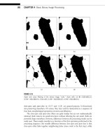
FIGURE 4.17
Close-open and open-close filtering of the binary image “cells.” Close-open with: (a)
B ϭ SQUARE(25); (b) B ϭ SQUARE(81); Open-close with: (c) B ϭ SQUARE(25); (d) B ϭ
SQUARE(81).
open-close often links neighboring objects together (since dilate is the first step). The
differences are usually somewhat subtle, yet often visible upon close inspection.
Figure 4.17 shows the result of applying the close-open and the open-close filters to
the ongoing binary image example. As can be seen, the results (for B fixed) are very
similar, although the close-open filtered results are somewhat cleaner, as expected. There
are also only small differences between the results obtained using the medium and larger
windows because of the intense smoothing that is occurring. To fully appreciate the
power of these smoothers, it is worth comparing to the original binarized image “cells”
in Fig. 4.13(a).

90 CHAPTER 4 Basic Binary Image Processing
The reader may wonder whether further sequencing of the filtered responses w i ll
produce different results. If the filters are properly alternated as in the construction
of the close-open and open-close filters, then the dual filters become increasingly similar.
However, the smoothing power can most easily be increased by simply taking the window
size to be larger.
Once again, the close-open and open-close filters are dual filters under compleme-
ntation.
We now return to the final binary smoothing filter, the majority filter. The majority
filter is also known as the binary median filter, since it may be regarded as a special case
(the binary case) of the gray level median filter (Chapter 12).
The majority filter has similar attributes as the close-open and open-close filters:
it removes too-small objects, holes, gaps, bays, and peninsulas (both ‘1’-valued and
‘0’-valued small features), and it also does not generally change the size of objects or
of background, as depicted in Fig. 4.18. It is less biased than any of the other morpho-
logical filters, since it does not have an initial erode or dilate operation to set the bias. In
fact, majority is its own dual under complementation, since
majority( f ,B) ϭ NOT{majority[NOT( f ),B]}. (4.29)
The majority filter is a powerful, unbiased shape smoother. However, for a given filter
size, it does not have the same degree of smoothing power as close-ope n or open-close.
Figure 4.19 shows the result of applying the majority or binary median filter to the
image “cell.” As can be seen, the results obtained are very smooth. Comparison with
the results of open-close and close-open are favorable, since the boundaries of the major
smoothed objects are much smoother in the case of the median filter, for both window
shapes used and for each size. The majority filter is quite commonly used for smoothing
noisy binary images of this type because of these nice properties. The more general gray
level median filter (Chapter 12) is also among the most used image processing filters.
4.4.4 Morphological Boundary Detection
The morphological filters are quite effective for smoothing binary images but they have
other important applications as well. One such application is boundary detection, which

is the binary case of the more general edge detectors studied in Chapters 19 and 20.
majority
FIGURE 4.18
Effect of majority filtering. The smallest holes, gaps, fingers, and extraneous objects are
eliminated.
4.4 Binary Image Morphology 91
(a) (b)
(c) (d)
FIGURE 4.19
Majority or median filtering of the binary image “cells.” Majority with: (a) B ϭ SQUARE(9); (b) B ϭ
SQUARE(25); Majority with (c) B ϭ SQUARE(81); (d) B ϭ CROSS(9).
At first glance, boundary detection may seem trivial, since the boundary points can
be simply defined as the transitions from ‘1’ to ‘0’ (and vice versa). However, when there
is noise present, boundary detection becomes quite sensitive to small noise artifacts,
leading to many useless detected edges. Another approach which allows for smoothing
of the object boundaries involves the use of mor phological operators.
The “difference” between a binary image and a dilated (or eroded) version of it is
one effective way of detecting the object boundaries. Usually it is best that the window B
that is used be small, so that the difference between image and dilation is not too large
(leading to thick, ambiguous detected edges). A simple and effective “difference” measure
92 CHAPTER 4 Basic Binary Image Processing
(a) (b)
FIGURE 4.20
Object boundary detection. Application of boundary(f , B) to (a) the image “cells”; (b) the majority-
filtered image in Fig. 4.19(c).
is the two-input exclusive-OR operator XOR. The XOR takes logical value ‘1’ only if its
two inputs are different. The boundary detector then becomes simply:
boundary( f ,B) ϭ XOR[f , dilate(f ,B)]. (4.30)
The result of this operation as applied to the binary image “cells” is shown in Fig. 4.20(a)
using B ϭ SQUARE(9). As can be seen, essentially all of the BLACK/WHITE transi-

tions are marked as boundary points. Often this is the desired result. However, in
other instances, it is desired to detect only the major object boundary points. This
can be accomplished by first smoothing the image with a close-ope n, open-close, or
majority filter. The result of this smoothed b oundary detection process is shown in
Fig. 4.20(b). In this case,the result is much cleaner, as only the major boundary points are
discovered.
4.5 BINARY IMAGE REPRESENTATION AND COMPRESSION
In several later chapters, methods for compressing gray level images are studied in
detail. Compressed images are representations that require less storage than the nomi-
nal storage. This is generally accomplished by coding of the data based on measured
statistics, rearrangement of the data to exploit patterns and redundancies in the data,
and (in the case of lossy compression) quantization of information. The goal is that
the image, when decompressed, either looks very much like the original despite a loss
4.5 Binary Image Representation and Compression 93
of some information (lossy compression), or is not different from the original (lossless
compression).
Methods for lossless compression of images are discussed in Chapter 16. Those
methods can generally be adapted to both gray level and binary images. Here, we will look
at two methods for lossless binary image representation that exploit an assumed struc-
ture for the images. In both methods the image data is represented in a new format that
exploits the structure. The first method is run-length coding, which is so-called because
it seeks to exploit the redundancy of long run-lengths or runs of constant value ‘1’ or ‘0’
in the binary data. It is thus appropriate for the coding/compression of binary images
containing large areas of constant value ‘1’ and ‘0.’ The second method, chain coding, is
appropriate for binary images containing binary contours, such as the boundary images
shown in Fig. 4.20. Chain coding achieves compression by exploiting this assumption.
The chain code is also an information-rich, highly manipulable representation that can
be used for shape analysis.
4.5.1 Run-Length Coding
The number of bits required to naively store a N ϫM binary image is NM. This can be

significantly reduced if it is known that the binary image is smooth in the sense that it is
composed primarily of large areas of constant ‘1’ and/or ‘0’ value.
The basic method of run-length coding is quite simple. Assume that the binary image
f is to be stored or transmitted on a row-by-row basis. Then for each image row numbered
m, the following algorithm steps are used:
1. Store the first pixel value (‘0’ or ‘1’) in row m in a 1-bit buffer as a reference;
2. Set the run counter c ϭ1;
3. For each pixel in the row:
– Examine the next pixel to the right;
– If it is the same as the current pixel, set c ϭc ϩ 1;
– If different from the current pixel, store c in a buffer of length b and
set c ϭ 1;
– Continue until end of row is reached.
Thus, each run-length is stored using b bits. This requires that an overall buffer with
segments of lengths b be reserved to store the run-lengths. Run-length coding yields
excellent lossless compressions, provided that the image contains lots of constant runs.
Caution is necessary, since if the image contains only very short runs, then run-length
coding can actually increase the required storage.
Figure 4.21 depicts two hypothetical image rows. In each case, the first symbol stored
in a 1-bit buffer will be logical ‘1.’ The run-length code for Fig. 4.21(a) would be ‘1,’ 7, 5,
8, 3, 1 with symbols after the ‘1’ stored using b bits. The first five runs in this sequence
94 CHAPTER 4 Basic Binary Image Processing
(a)
(b)
FIGURE 4.21
Example rows of a binary image, depicting (a) reasonable and (b) unreasonable scenarios for
run-length coding.
have average length 24/5ϭ 4.8, hence if b Յ4, then compression will occur. Of course,
the compression can be much higher, since there may be runs of lengths in the dozens or
hundreds, leading to very high compressions.

In Fig. 4.21(b), however, in this worst-case example, the storage actually increases
b-fold! Hence, care is needed when applying this method. The apparent rule, if it can
be applied a priori, is that the average run-length L of the image should satisfy L > b if
compression is to occur. In fact, the compression ratio will be approximately L/b.
Run-length coding is also used in other scenarios than binary image coding. It can
also be adapted to situations where there are run-lengths of any value. For example, in the
JPEG lossy image compression standard for gray level images (see Chapter 17), a form
of run-length coding is used to code runs of zero-valued frequency-domain coefficients.
This run-length coding is an important factor in the good compression performance of
JPEG. A more abstract form of run-length coding is also responsible for some of the
excellent compression performance of recently developed wavelet image compression
algorithms (Chapters 17 and 18).
4.5.2 Chain Coding
Chain coding is an efficient representation of binary images composed of contours. We
will refer to these as “contour images.” We assume that contour images are composed
only of single-pixel width, connected contours (straight or curved). These arise from
processes of edge detection or boundary detection, such as the morphological boundary
detection method just described above, or the results of some of the edge detectors
described in Chapters 19 and 20 when applied to grayscale images.
The basic idea of chain coding is to code contour directions instead of naïve bit-by-bit
binary image coding or even coordinate representations of the contours. Chain coding is
based on identifying and storing the directions from each pixel to its neighbor pixel on
each contour. Before defining this process, it is necessary to clarify the various ty pes of
neighbors that are associated with a given pixel in a binary image. Figure 4.22 depicts two
neighborhood systems around a pixel (shaded). To the left are depicted the 4-neighbors
of the pixel, which are connected along the horizontal and vertical directions. The set
of 4-neighbors of a pixel located at coordinate n will be denoted N
4
(n). To the r ight
4.5 Binary Image Representation and Compression 95

FIGURE 4.22
Depiction of the 4-neighbors and the 8-neighbors of a pixel (shaded).
Contour
Initial point
and directions
(a) (b)
0
1
2
3
4
5
6
7
FIGURE 4.23
Representation of a binary contour by direction codes. (a) A connected contour can be repre-
sented exactly by an initial point and the subsequent directions; (b) only 8 direction codes are
required.
are the 8-neighbors of the shaded pixel in the center of the grouping. These include the
pixels connected along the diagonal directions. The set of 8-neighbors of a pixel located
at coordinate n will be denoted N
8
(n).
If the initial coordinate n
0
of an 8-connected contour is known, then the rest of the
contour can be represented without loss of information by the directions along which the
contour propagates, as depicted in Fig. 4.23(a). The initial coordinate can be an endpoint,
if the contour is open, or an arbitrary point, if the contour is closed. The contour can be
reconstructed from the directions, if the initial coordinate is known. Since there are only

eight directions that are possible, then a simple 8-neighbor direction code may be used.
The integers {0, ,7}suffice for this, as shown in Fig. 4.23(b).
Of course, the direction codes 0,1, 2,3,4,5, 6, 7 can be represented by their 3-bit binary
equivalents: 000, 001,010,011,100,101,110, 111. Hence, each point on the contour after
the initial point can be coded by three bits. The initial point of each contour requires
log
2
(MN ) bits, where · denotes the ceiling function: x ϭ the smallest integer that
is greater than or equal to x. For long contours, storage of the initial coordinates is
incidental.
Figure 4.24 shows an example of chain coding of a short contour. After the initial
coordinate n
0
ϭ (n
0
,m
0
) is stored, the chain code for the remainder of the con-
tour is: 1,0,1,1,1, 1, 3, 3,3,4,4,5,4 in integer format, or 001,000,001,001,001,001, 011,
011,011,100,100,101,100 in binary format.
96 CHAPTER 4 Basic Binary Image Processing
m
0
5
Initial point
n
0
FIGURE 4.24
Depiction of chain coding.
Chain coding is an efficient representation. For example, if the image dimensions are

N ϭM ϭ 512, then representing the contour by storing the coordinates of each contour
point requires six times as much storage as the chain code.
CHAPTER
5
Basic Tools for Image
Fourier Analysis
Alan C. Bovik
The University of Texas at Austin
5.1 INTRODUCTION
In this third chapter on basic methods, the basic mathematical and algorithmic tools for
the frequency domain analysis of digital images are explained. Also, 2D discrete-space
convolution is introduced. Convolution is the basis for linear filtering, which plays
a central role in many places in this Guide. An understanding of frequency domain
and linear filtering concepts is essential to be able to comprehend such significant
topics as image and video enhancement, restoration, compression, segmentation, and
wavelet-based methods. Explor ing these ideas in a 2D setting has the advantage that
frequency domain concepts and transforms can be visualized as images, often enhancing
the accessibility of ideas.
5.2 DISCRETE-SPACE SINUSOIDS
Before defining any frequency-based transforms, first we shall explore the concept of
image frequency, or more generally, of 2D frequency. Many readers may have a basic
background in the frequency domain analysis of 1D signals and systems. The basic
theories in two dimensions are founded on the same principles. However, there are
some extensions. For example, a 2D frequency component, or sinusoidal function, is
characterized not only by its location (phase shift) and its frequency of oscillation but
also by its direction of oscillation.
Sinusoidal functions will play an essential role in all of the developments in this
chapter. A 2D discrete-space sinusoid is a function of the form
sin[2␲(Um ϩ Vn)]. (5.1)
Unlike a 1D sinusoid, the function (5.1) has two frequencies, U and V (with units of

cycles/pixel) which represent the frequency of oscillation along the vertical (m) and
97
98 CHAPTER 5 Basic Tools for Image Fourier Analysis
horizontal (n) spatial image dimensions. Generally, a 2D sinusoid oscillates (is non con-
stant) along every direction except for the direction orthogonal to the direction of fastest
oscillation. The frequency of this fastest oscillation is the radial frequency:
⍀ϭ

U
2
ϩ V
2
, (5.2)
which has the same units as U and V , and the direction of this fastest oscillation is the
angle:
␪ ϭ tan
Ϫ1

V
U

(5.3)
with units of radians. Associated with (5.1) is the complex exponential function
exp [j2␲(Um ϩ Vn)] ϭ cos[2␲(Um ϩ Vn)]ϩ jsin[2␲(Um ϩ Vn)], (5.4)
where j ϭ
√
Ϫ1 is the pure imaginary number.
In general, sinusoidal functions can be defined on discrete integer grids, hence (5.1)
and (5.4) hold for all integers — < m, n <. However, sinusoidal functions of infinite
duration are not encountered in practice, although they are useful for image modeling

and in certain image decompositions that we will explore.
In practice, discrete-space images are confined to finite M ϫ N sampling grids, and
we will also find it convenient to utilize finite-extent (M ϫ N ) 2D discrete-space sinusoids
which are defined only for integers
0 Յ m Յ M Ϫ 1, 0 Յ n Յ N Ϫ 1, (5.5)
and undefined elsewhere. A sinusoidal function that is confined to the domain (5.5) can
be contained within an image matrix of dimension M ϫ N ,and is thus easily manipulated
digitally.
In the case of finite sinusoids defined on finite grids (5.5) it will often be convenient
to use the scaled frequencies
(u,v) ϭ (MU ,NV ), (5.6)
which have the visually intuitive units of cycles/image. With this, the 2D sinusoid (5.1)
defined on finite grid (5.5) can be re-expressed as:
sin

2␲

u
M
m ϩ
v
N
n

(5.7)
with similar redefinition of the complex exponential (5.4).
Figure 5.1 depicts several discrete-space sinusoids of dimensions 256 ϫ 256 displayed
as intensity images after linear mapping the grayscale of each to the range 0Ϫ255. Because
of the nonlinear response of the eye, the functions in Fig. 5.1 look somewhat more
like square waves than smoothly-varying sinusoids, particularly at higher frequencies.

However, if any of the images in Fig. 5.1 is sampled along a straight line of arbitrary
orientation, the result is an ideal (sampled) sinusoid.
A peculiarity of discrete-space (or discrete-time) sinusoids is that they have a maxi-
mum possible physical frequency at which they can oscillate. Although the frequency
variables (u,v)or(U , V ) may be taken arbitrarily large, these large values do not
5.2 Discrete-Space Sinusoids 99
(c) (d)
(b)(a)
FIGURE 5.1
Examples of finite 2D discrete-space sinusoidal functions. The scaled frequencies (5.6)
measured in cycles/image are (a) u ϭ 1, v ϭ 4; (b) u ϭ 10, v ϭ 5; (c) u ϭ 15, v ϭ 35; and (d)
u ϭ 65, v ϭ 35.
correspond to arbitrarily large physical oscillation frequencies. The ramifications of
this are quite deep and significant and relate to the restrictions placed on sampling
of continuous-space images (the Sampling Theorem) and the Nyquist frequency.
As an example of this principle we will study a 1D example of a discrete sinusoid.
Consider the finite cosine function cos

2␲

u
M
m ϩ
v
N
n

ϭ cos

2␲

u
16
m

which results
by taking M ϭ N ϭ 16, and v ϭ 0. This is a cosine wave propagating in the m-direction
only (all columns are the same) at frequency u (cycles/image).
Figure 5.2 depicts the 1D cosine for various values of u. As can be seen, the physical
oscillation frequency increases until u ϭ 8; for incrementally larger values of u,however,
the physical frequency diminishes. In fact, the function is period-16 in the frequency
index u:
cos

2␲
u
16
m

ϭ cos

2␲
(
u ϩ 16k
)
16
m

(5.8)
100 CHAPTER 5 Basic Tools for Image Fourier Analysis
u 5 2 u 5 14or

u 5 4 u 5 12
or
1614121086420
0
1
m
1614121086420
21
0
1
m
u 5 1
u 5 15
or
1614121086420
21
0
1
m
1614121086420
21
0
1
m
21
u 5 8
FIGURE 5.2
Illustration of physical versus numerical frequencies of discrete-space sinusoids.
for all integers k. Indeed, the highest physical frequency of cos


2␲
u
M
m

occurs at u ϭ
M/2 ϩ kM (for M even) for all integers k. At these periodically-placed frequencies,
(5.8) is equal to (Ϫ1)
m
; the fastest discrete-index oscillation is the alternating signal.
This obser vation will be important next as we define the various frequency domain
image transforms.
5.3 DISCRETE-SPACE FOURIER TRANSFORM
The discrete-space Fourier transform (DSFT) of a given discrete-space image f is given by
F(U ,V ) ϭ
ϱ

mϭϪϱ
ϱ

nϭϪϱ
f (m,n)e
Ϫj2␲(UmϩVn)
(5.9)
with inverse discrete-space Fourier transform (IDSFT):
f (m,n) ϭ
0.5

Ϫ0.5
0.5


Ϫ0.5
F(U ,V )e
j2␲(UmϩVn)
dU dV . (5.10)
When (5.9) and (5.10) hold, we will often make the notation f

↔
F and say that f ,F form
a DSFT pair. The units of the frequencies (U, V )in(5.9) and (5.10) are cycles/pixel. It
5.3 Discrete-Space Fourier Transform 101
should be noted that, unlike continuous Fourier transforms, the DSFT is asymmetrical
in that the forward transform F is continuous in the frequency variables (U ,V ), while
the image or inverse transform is discrete. Thus, the DSFT is defined as a summation,
while the IDSFT is defined as an integral.
There are several ways of interpreting the DSFT (5.9) and (5.10). The most usual
mathematical interpretation of (5.10) is as a decomposition of f (m,n) into or thonormal
complex exponential basis functions e
j2␲(UmϩVn)
that satisfy
0.5

Ϫ0.5
0.5

Ϫ0.5
e
j2␲(UmϩVn)
e
Ϫj2␲(UpϩVq)

dU dV ϭ

1; m ϭ p and n ϭ q
0 ; else
. (5.11)
Another (somewhat less precise) interpretation is the engineering concept of the trans-
formation, without loss, of space domain image information into frequency domain
image information. Representing the image information in the frequency domain has
significant conceptual and algorithmic advantages, as will be seen. A third interpre-
tation is a physical one, where the image is viewed as the result of a sophisticated
constructive-destructive interference wave pattern. By assigning each of the infinite num-
ber of complex exponential wave functions e
j2␲(UmϩVn)
with the appropriate complex
weights F(U ,V ), the intricate structure of any discrete-space image can be recreated
exactly as an interference-sum.
The DSFT possesses a number of important properties that will be useful in defining
applications. In the following, assume that f

↔
F, g

↔
G, and h

↔
H.
5.3.1 Linearity of DSFT
Given images f ,g and arbitrary complex constants a,b, the following holds:
af ϩ bg


↔
aF ϩ bG. (5.12)
This property of linearity follows directly from (5.9), and can be extended to a weighted
sum of any countable number of images. It is fundamental to many of the properties of,
and operations involving, the DSFT.
5.3.2 Inversion of DSFT
The 2D function F(U , V ) uniquely satisfies the relationships (5.9) and (5.10). That the
inversion holds can be easily shown by substituting (5.9) into (5.10), reversing the order
of sum and integral, and then applying (5.11).
5.3.3 Magnitude and Phase of DSFT
The DSFT F of an image f is generally complex-valued. As such it can be written in the
form
F(U ,V ) ϭ R(U ,V ) ϩ jI (U , V ), (5.13)
102 CHAPTER 5 Basic Tools for Image Fourier Analysis
where
R(U ,V ) ϭ
ϱ

mϭϪϱ
ϱ

nϭϪϱ
f (m,n) cos[2␲(Um ϩ Vn)] (5.14)
and
I(U , V ) ϭϪ
ϱ

mϭϪϱ
ϱ


nϭϪϱ
f (m,n) sin[2␲(Um ϩ Vn)] (5.15)
are the real and imaginary parts of F(U ,V ), respectively.
The DSFT can also be written in the often-convenient phasor form
F(U ,V ) ϭ |F(U ,V )|e
j∠ F (U ,V )
, (5.16)
where the magnitude spectrum of image f is
|F(U ,V )|ϭ

R
2
(
U , V
)
ϩ I
2
(
U , V
)
(5.17)
ϭ

F
(
U , V
)
F
∗

(
U , V
)
, (5.18)
where ‘∗’ denotes the complex conjugation. The phase spectrum of image f is
∠F(U ,V ) ϭ tan
Ϫ1

I
(
U , V
)
R
(
U , V
)

. (5.19)
5.3.4 Symmetry of DSFT
If the image f is real, which is usually the case, then the DSFT is conjugate symmetric:
F(U ,V ) ϭ F
∗
(ϪU , ϪV ), (5.20)
which means that the DSFT is completely specified by its values over any half-plane.
Hence, if f is real, the DSFT is redundant. From (5.20), it follows that the magnitude
spectrum is even symmetric:
|F(U ,V )|ϭ |F(ϪU ,ϪV )|, (5.21)
while the phase spectrum is odd symmetric:
∠F(U ,V ) ϭϪ∠F(ϪU ,ϪV ). (5.22)
5.3.5 Translation of DSFT

Multiplying (or modulating) the discrete-space image f (m, n) by a 2D complex expo-
nential wave function exp[j2␲(U
0
m ϩ V
0
n)] results in a translation of the DSFT:
f (m,n) exp[j2␲(U
0
m ϩ V
0
n)]

↔
F(U–U
0
,V–V
0
). (5.23)
Likewise, translating the image f by amounts m
0
and n
0
produces a modulated DSFT:
f (m Ϫ m
0
,n Ϫ n
0
)

↔

F(U ,V )exp[Ϫj2␲(Um
0
ϩ Vn
0
)]. (5.24)
5.4 2D Discrete Fourier Transform (DFT) 103
5.3.6 Convolution and the DSFT
Given two images or 2D functions f and h, their 2D disc rete-space linear convolution is
given by
g (m,n) ϭ f (m,n) ∗h(m,n) ϭ h(m,n) ∗f (m,n) ϭ
ϱ

pϭϪϱ
ϱ

qϭϪϱ
f (p,q)h(m Ϫ p,n Ϫ q). (5.25)
The linear convolution expresses the result of passing an image signal f through a 2D
linear convolution system h (or vice versa). The commutativity of the convolution is
easily seen by making a substitution of variables in the double sum in (5.25).
If g , f , and h satisfy the spatial convolution relationship (5.25), then their DSFT’s
satisfy
G(U, V ) ϭ F (U , V )H(U ,V ), (5.26)
hence convolution in the space domain corresponds directly to multiplication in the
spatial frequency domain. This important property is significant both conceptually, as
a simple and direct means for effecting the frequency content of an image, and com-
putationally, since the linear convolution has such a simple expression in the frequency
domain.
The 2D DSFT is the basic mathematical tool for analyzing the frequency domain
content of 2D discrete-space images. However, it has a major drawback for digital

image processing applications: the DSFT F(U ,V ) of a discrete-space image f (m,n)
is continuous in the frequency coordinates (U , V ); there are an uncountably infinite
number of values to compute. As such, discrete (digital) processing or display in the
frequency domain is not possible using the DSFT unless it is modified in s ome way.
Fortunately, this is possible when the image f is of finite dimensions. In fact, by sampling
the DSFT in the frequency domain we are able to create a computable Fourier-domain
transform.
5.4 2D DISCRETE FOURIER TRANSFORM (DFT)
Now we restrict our attention to the practical case of discrete-space images that are
of finite extent. Hence assume that image f (m,n) can be expressed as a matrix f ϭ
[f (m,n),0Յ m Յ M Ϫ 1,0 Յ n Յ N Ϫ 1]. As we will show, a finite-extent image matrix
f can be represented exactly as a finite weighted sum of 2D frequency components,
instead of an infinite number. This leads to computable and numerically manipulable
frequency domain representations. Before showing how this is done, we shall introduce
a special notation for the complex exponential that w ill simplify much of the ensuing
development.
We will use
W
K
ϭ exp

Ϫj
2␲
K

(5.27)
104 CHAPTER 5 Basic Tools for Image Fourier Analysis
as a shorthand for the basic complex exponential, where K is the dimension along one
of the image axes (K ϭN or K ϭM ). The notation (5.27) makes it possible to index the
various elementary frequency components at arbitrary spatial and frequency coordinates

by simple exponentiation:
W
um
M
W
vn
N
ϭ cos

2␲

u
M
m ϩ
v
N
n

Ϫ j sin

2␲

u
M
m ϩ
v
N
n

. (5.28)

This process of space and frequency indexing by exponentiation greatly simplifies the
manipulation of frequency components and the definition of the discrete Fourier trans-
form (DFT). Indeed, it is possible to develop frequency domain concepts and frequency
transforms without the use of complex numbers (and in fact some of these, such as the
discrete cosine transform, or DCT, are widely used, especially in image compression—
See Chapters 16 and 17 of this Guide).
For the purpose of analysis and basic theory, it is much simpler to use W
um
M
and W
vn
N
to represent finite-extent (of dimensions M and N ) frequency components oscillating at
u (cycles/image) and v (cycles/image) in the m- and n-directions, respectively. Clearly,


W
um
M
W
vn
N


ϭ 1 (5.29)
and
∠W
um
M
W

vn
N
ϭϪ2␲

u
M
m ϩ
v
N
n

. (5.30)
Observe that the minimum physical frequency of W
um
M
periodically occurs at the indices
u ϭ kM for all integers k:
W
kMm
M
ϭ 1 (5.31)
for any integer m; the minimum oscillation is no oscillation. If M is even, the maximum
physical frequency periodically occurs at the indices u ϭ kM ϩ M /2:
W
(
kMϩM /2
)
m
M
ϭ 1 ·e

Ϫj␲m
ϭ (Ϫ1)
m
, (5.32)
which is the discrete period-2 (alternating) function, the highest possible discrete
oscillation frequency.
The 2D DFT of the finite-extent (M ϫ N ) image f is given by
˜
F
(
u,v
)
ϭ
MϪ1

mϭ0
N Ϫ1

nϭ0
f (m,n)W
um
M
W
vn
N
(5.33)
for integer frequencies 0ՅuՅM Ϫ1,0Յv ՅN Ϫ1. Hence the DFT is also of finite-extent
M ϫ N , and can be expressed as a (generally complex-valued) matrix
˜
F ϭ [

˜
F
(
u,v
)
;0Յ
u Յ M Ϫ 1,0 Յ v Յ N Ϫ 1]. It has a unique inverse discrete Fourier transform,orIDFT :
f (m,n) ϭ
1
MN
MϪ1

uϭ0
N Ϫ1

vϭ0
˜
F
(
u,v
)
W
Ϫum
M
W
Ϫvn
N
(5.34)
5.4 2D Discrete Fourier Transform (DFT) 105
for 0 Յ m Յ M Ϫ 1, 0 Յ n Յ N Ϫ 1. When (5.33) and (5.34) hold, it is often denoted

f
DFT
↔
˜
F and we say that f,
˜
F form a DFT pair.
A number of observations regarding the DFT and its relationship to the DSFT are
necessary. First, the DFT and IDFT are symmetrical, since both forward and inverse
transforms are defined as sums. In fact they have the same form, except for the polarity
of the exponents and a scaling factor. Secondly, both forward and inverse transforms are
finite sums; both
˜
F and f can be represented uniquely as finite weighted sums of finite-
extent complex exponentials with integer-indexed frequencies. Thus, for example, any
256 ϫ 256 digital image can be expressed as the weighted sum of 256
2
ϭ 65,536 complex
exponential (sinusoid) functions including those with real parts shown in Fig. 5.1. Note
that the frequencies (u,v) are scaled so that their units are in cycles/image, as in (5.6) and
Fig. 5.1.
Most importantly, the DFT has a direct relationship to the DSFT. In fact, the DFT of
an M ϫ N image f is a uniformly sampled version of the DSFT of f:
˜
F
(
u,v
)
ϭ F(U , V )





U ϭ
u
M
,V ϭ
v
N
(5.35)
for integer frequency indices 0 Յ u Յ M Ϫ 1,0 Յ v Յ N Ϫ 1. Since f is of finite extent,
and contains MN elements, the DFT
˜
F is conservative in that it also requires only MN
elements to contain complete information about f (to be exactly invertible). Also, since
˜
F is simply e venly-spaced samples of F, many of the properties of the DSFT translate
directly with little or no modification to the DFT.
5.4.1 Linearity and Invertibility of DFT
The DFT is linear in the sense of (5.12). It is uniquely invertible, as can be established by
substituting (5.33) into (5.34), reversing the order of summation, and using the fact that
the discrete complex exponentials are also orthogonal
MϪ1

uϭ0
N Ϫ1

vϭ0

W

um
M
W
Ϫup
M

W
vn
N
W
Ϫvq
N

ϭ

MN ; m ϭ p and n ϭ q
0 ; else
. (5.36)
The DFT matrix
˜
F is generally complex, hence it has an associated magnitude
spectrum matrix, denoted
|
˜
F| ϭ [|
˜
F
(
u,v
)

|;0Յ u Յ M Ϫ 1, 0 Յ v Յ N Ϫ 1] (5.37)
and phase spectrum matrix denoted
∠
˜
F ϭ [∠
˜
F
(
u,v
)
;0Յ u Յ M Ϫ 1, 0 Յ v Յ N Ϫ 1]. (5.38)
The elements of |
˜
F| and ∠
˜
F are computed in the same way as the DSFT magnitude and
phase (5.16)–(5.19).
106 CHAPTER 5 Basic Tools for Image Fourier Analysis
5.4.2 Symmetry of DFT
Like the DSFT, if f is real-valued, then the DFT matrix is conjugate symmetric, but in the
matrix sense:
˜
F
(
u,v
)
ϭ
˜
F
∗

(
M Ϫ u,N Ϫ v
)
(5.39)
for 0 Յ u Յ M Ϫ 1,0 Յ v Յ N Ϫ 1. This follows easily by substitution of the reversed and
translated frequency indices (M Ϫ u,N Ϫ v) into the forward DFT equation (5.33).An
apparent repercussion of (5.39) is that the DFT
˜
F matrix is redundant, and hence can
represent the M ϫ N image with only about MN/2 DFT coefficients. This mystery is
resolved by realizing that
˜
F is complex-valued, hence it requires twice the storage for real
and imaginar y components. If f is not real-valued, then (5.39) does not hold.
Of course, (5.39) implies symmetries of the magnitude and phase spectra:
|
˜
F
(
u,v
)
| ϭ |
˜
F
(
M Ϫ u,N Ϫ v
)
| (5.40)
and
∠

˜
F
(
u,v
)
ϭϪ∠
˜
F
(
M Ϫ u,N Ϫ v
)
(5.41)
for 0 Յ u Յ M Ϫ 1,0 Յ v Յ N Ϫ 1.
5.4.3 Periodicity of DFT
Another property of the DSFT that carries over to the DFT is frequency periodicity. Recall
that the DSFT F(U ,V ) has unit period in U and V . The DFT matrix
˜
F was defined to be
of finite-extent M ϫ N. However, the forward DFT equation (5.33) admits the possibility
of evaluating
˜
F
(
u,v
)
outside of the range 0 Յ u Յ M Ϫ 1,0 Յ v Յ N Ϫ 1. It turns out that
˜
F
(
u,v

)
is period-M and period-N along the u and v dimensions, respectively. For any
integers k,l:
˜
F
(
u ϩ kM ,v ϩ lN
)
ϭ
˜
F
(
u,v
)
(5.42)
for every 0 Յ u Յ M Ϫ 1, 0 Յ v Յ N Ϫ 1. This follows easily by substitution of the peri-
odically extended frequency indices (u ϩ kM, v ϩ lN ) into the forward DFT equation
(5.33). The interpretation (5.42) of the DFT is called the periodic extension of the DFT.
It is defined for all integer frequencies u,v.
Although many properties of the DFT are the same, or similar to those of the DSFT,
certain important properties are different. These effects arise from sampling the DSFT to
create the DFT.
5.4.4 Image Periodicity Implied by DFT
A seemingly innocuous, yet extremely important consequence of sampling the DSFT is
that the resulting DFT equations imply that the image f is itself periodic. In fact, the IDFT
equation (5.34) implies that for any integers k,l:
f (m ϩ kM,n ϩ lN) ϭ f (m, n) (5.43)
5.4 2D Discrete Fourier Transform (DFT) 107
for every 0 Յ m Յ M Ϫ 1,0 Յ n Յ N Ϫ 1. This follows easily by substitution of the peri-
odically extended space indices (m ϩ kM,n ϩ lN ) into the inverse DFT equation (5.34).

Clearly, finite-extent digital images arise from imaging the real world through finite
field of view (FOV) devices, such as cameras, and outside that FOV, the world does not
repeat itself periodically, ad infinitum. The implied periodicity of f is purely a synthetic
effect that derives from sampling the DSFT. Nevertheless, it is of paramount importance,
since any algorithm that is developed, and that uses the DFT, will operate as though
the DFT-transformed image were spatially periodic in the sense (5.43). One important
property and application of the DFT that is effected by this spatial periodicity is the
frequency-domain convolution property.
5.4.5 Cyclic Convolution Property of the DFT
One of the most significant properties of the DSFT is the linear convolution property
(5.25) and (5.26), which says that space domain convolution corresponds to frequency
domain multiplication:
f
∗
h

↔
FH. (5.44)
This useful property makes it possible to analyze and design linear convolution-based sys-
tems in the frequency domain. Unfortunately, property (5.44) does not hold for the DFT;
a product of DFT’s does not correspond (inverse transfor m) to the linear convolution
of the original DFT-transformed functions or images. However, it does correspond to
another type of convolution, variously known as cyclic convolution, circular convolution,
or wraparound convolution.
We will demonstrate the form of the cyclic convolution by deriving it. Consider the
two M ϫ N image functions f
DFT
↔
˜
F and h

DFT
↔
˜
H. Define the pointwise matrix product
1
˜
G ϭ
˜
F ⊗
˜
H (5.45)
according to
˜
G(u, v) ϭ
˜
F(u, v)
˜
H( u,v) (5.46)
for 0 Յ u Յ M Ϫ 1,0 Յ v Յ N Ϫ 1. Thus we are interested in the form of g.Foreach
0 Յ m Յ M Ϫ 1,0 Յ n Յ N Ϫ 1, we have
g (m,n) ϭ
1
MN
MϪ1

uϭ0
N Ϫ1

vϭ0
˜

G(u, v)W
Ϫum
M
W
Ϫvn
N
ϭ
1
MN
MϪ1

uϭ0
N Ϫ1

vϭ0
˜
F(u, v)
˜
H( u,v)W
Ϫum
M
W
Ϫvn
N
1
As opposed to the standard matrix product.
108 CHAPTER 5 Basic Tools for Image Fourier Analysis
ϭ
1
MN

MϪ1

uϭ0
N Ϫ1

vϭ0
⎧
⎨
⎩
MϪ1

pϭ0
N Ϫ1

qϭ0
f

p, q

W
up
M
W
vq
N
⎫
⎬
⎭
ϫ
⎧

⎨
⎩
MϪ1

rϭ0
N Ϫ1

sϭ0
h
(
r, s
)
W
ur
M
W
vs
N
⎫
⎬
⎭
W
Ϫum
M
W
Ϫvn
N
(5.47)
by substitution of the definitions of
˜

F(u,v) and
˜
H(u, v). Rearranging the order of the
summations to collect all of the complex exponentials inside the innermost summation
reveals that
g (m,n) ϭ
1
MN
MϪ1

pϭ0
N Ϫ1

qϭ0
f

p, q

MϪ1

rϭ0
N Ϫ1

sϭ0
h
(
r, s
)
MϪ1


uϭ0
N Ϫ1

vϭ0
W
u
(
pϩrϪm
)
M
W
v
(
qϩsϪn
)
N
. (5.48)
Now, from (5.36), the innermost summation
MϪ1

uϭ0
N Ϫ1

vϭ0
W
u
(
pϩrϪm
)
M

W
v
(
qϩsϪn
)
N
ϭ

MN ; r ϭ m Ϫ p and s ϭ n Ϫ q
0; else
(5.49)
hence
g (m,n) ϭ
MϪ1

pϭ0
N Ϫ1

qϭ0
f

p, q

h

m Ϫ p

M
,


n Ϫ q

N

(5.50)
ϭ f (m, n)  h(m, n) ϭ h(m, n)  f (m, n), (5.51)
where (x)
N
ϭ x mod N and the symbol ‘’ denotes the 2D cyclic convolution.
2
The final step of obtaining (5.50) from (5.49) follows since the argument of the
shifted and twice-reversed (along each axis) function h(m Ϫ p,n Ϫ q) finds no mean-
ing whenever (m Ϫ p)/∈{0, ,M Ϫ 1} or (n Ϫ q)/∈{0, ,N Ϫ 1}, since h is undefined
outside of those coordinates. However, because the DFT was used to compute g (m, n),
then the periodic extension of h(m Ϫ p,n Ϫ q) is implied, which can be expressed as
h

m Ϫ p

M
,

n Ϫ q

N

.Hence(5.50) follows. That‘’ is commutative and easily estab-
lished by a substitution of variables in (5.50). It can also be seen that cyclic convolution
is a form of linear convolution, but with one (either, but not both) of the two functions
being periodically extended. Hence

f (m,n)  h(m,n) ϭ f (m,n) ∗h[(m)
M
,(n)
N
] ϭ f [(m)
M
,(n)
N
]∗h(m,n). (5.52)
This cyclic convolution property of the DFT is unfortunate, since in the majority of
applications it is not desired to compute the cyclic convolution of two image functions.
Instead, what is frequently desired is the linear convolution of two functions, as in the
case of linear filtering. In both linear and cyclic convolution, the two functions are super-
imposed, with one function reversed along both axes and shifted to the point at which
2
Modular arithmetic is remaindering. Hence (x)
N
is the integer remainder of (x/N ).
5.4 2D Discrete Fourier Transform (DFT) 109
the convolution is being computed. The product of the functions is computed at every
point of overlap, with the sum of products being the convolution. In the case of the cyclic
convolution, one (not both) of the functions is periodically extended, hence the overlap
is much larger and wraps around the image boundaries. This produces a significant error
with respect to the correct linear convolution result. This error is called spat ial aliasing,
since the wraparound error contributes false information to the convolution sum.
Figure 5.3 depicts the linear and cyclic convolutions of two hypothetical M ϫ N
images f and h at a point (m
0
,n
0

). From the figure, it can be seen that the wraparound
Image f Image h
(m
0
, n
0
)
(m
0
, n
0
)
(m
0
, n
0
)
(0, 0)
(0, 0)
(0, 0)
(0, 0)
(a)
(b)
(c)
FIGURE 5.3
Convolution of two images. (a) Images f and h; (b) linear convolution result at (m
0
,n
0
) is computed

as the sum of products where f and h overlap; (c) cyclic convolution result at (m
0
,n
0
) is computed
as the sum of products where f and the periodically extended h overlap.
110 CHAPTER 5 Basic Tools for Image Fourier Analysis
error can overwhelm the linear convolution contribution. Note in Fig. 5.3(b) that
although the linear convolution sum (5.25) extends over the indices 0 Յ m Յ M Ϫ 1
and 0 Յ n Յ N Ϫ 1, the overlap is restricted to the indices.
5.4.6 Linear Convolution Using the DFT
Fortunately, it turns out that it is possible to compute the linear convolution of two
arbitr ary finite-extent 2D discrete-space functions or images using the DFT. The process
requires modifying the functions to be convolved prior to taking the product of their
DFT’s. The modification acts to cancel the effects of spatial aliasing.
Suppose more generally that f and h are two arbitrary finite-extent images of
dimensions M ϫ N and P ϫ Q, respectively. We are interested in computing the lin-
ear convolution g ϭ f
∗
h using the DFT. We assume the general case where the images
f , h do not have the same dimensions, since in most applications an image is convolved
with a filter function of different (usually much smaller) extent.
Clearly,
g (m,n) ϭ f (m,n)
∗
h(m,n) ϭ
MϪ1

pϭ0
N Ϫ1


qϭ0
f (p,q)h(m Ϫ p,n Ϫ q). (5.53)
Inverting the pointwise products of the DFT’s
˜
F ⊗
˜
H will not lead to (5.53), since
wraparound error will occur. To cancel the wraparound error, the functions f and h
are modified by increasing their size by zero-padding them. Zero-padding means that
the arrays f and h are expanded into larger arrays, denoted
ˆ
f and
ˆ
h, by filling the empty
spaces with zeroes. To compute the linear convolution, the pointwise product
˜
ˆ
G =
˜
ˆ
F ⊗
˜
ˆ
H
of the DFTs of the zero-padded functions
ˆ
f and
ˆ
h is computed. The inverse DFT ˆg of

˜
ˆ
G
then contains the correct linear convolution result.
The question remains as to how many zeroes are used to pad the functions f and
h. The answer to this lies in understanding how zero-padding works and how large the
linear convolution result should be. Zero-padding acts to cancel the spatial aliasing error
(wraparound) of the DFT by supplying zeroes where the wraparound products occur.
Hence the wraparound products are all zero and contribute nothing to the convolution
sum. This leaves only the linear convolution contribution to the result. To understand
how many zeroes are needed, it must be realized that the resulting product DFT
˜
ˆ
G
corresponds to a periodic function ˆg. If the horizontal/vertical periods are too small
(not enough zero-padding), the periodic replicas will overlap (spatial aliasing). If the
periods are just large enough, then the periodic replicas will be contiguous instead of
overlapping, hence spatial aliasing will be canceled. Padding with more zeroes than this
results in excess computation. Figure 5.4 depicts the successful result of zero-padding to
eliminate wraparound error.
The correct period lengths are equal to the lengths of the correct linear convolution
result. The linear convolution result of two arbitrary M ϫ N and P ϫ Q image functions
will generally be (M ϩ P Ϫ 1) ϫ (N ϩ Q Ϫ 1), hence we would like the DFT
˜
ˆ
G to have
5.4 2D Discrete Fourier Transform (DFT) 111
0
0
(a)

(b)
Zero-padded
image f
ˆˆ
Zero-padded
image h
(m
0
, n
0
)
FIGURE 5.4
Linear convolution of the same two images as Fig. 5.2 by zero-padding and cyclic convolution
(via the DFT). (a) Zero-padded images
ˆ
f and
ˆ
h; (b) cyclic convolution at (m
0
, n
0
) computed as
the sum of products where
ˆ
f and the periodically extended
ˆ
h overlap. These products are zero
except over the range 0 Յ p Յ m
0
and 0 Յ q Յ n

0
.
these dimensions. Therefore, the M ϫ N function f and the P ϫ Q function h must
both be zero-padded to size (M ϩ P Ϫ 1) ϫ (N ϩ Q Ϫ 1). This yields the correct linear
convolution result:
ˆg ϭ
ˆ
f 
ˆ
h ϭ f
∗
h. (5.54)
In most cases, linear convolution is performed between an image and a filter function
much smaller than the image: M >> P and N >> Q. In such cases the result is not much
larger than the image, and often only the M ϫ N portion indexed 0 Յ m Յ M Ϫ 1,0 Յ
n Յ N Ϫ 1 is retained. The reason behind this is, firstly, it may be desirable to retain
images of size MN only, and secondly, the linear convolution result beyond the borders
112 CHAPTER 5 Basic Tools for Image Fourier Analysis
of the original image may be of little interest, since the original image was zero there
anyway.
5.4.7 Computation of the DFT
Inspection of the DFT relation (5.33) reveals that computation of each of the MN DFT
coefficients requires on the order of MN complex multiplies/additions. Hence, on the
order of M
2
N
2
complex,multiplies and additions are needed to compute the overall DFT
of an M ϫ N image f. For example,if M ϭ N ϭ512, then on the order of 2
36

ϭ 6.9 ϫ 10
10
complex multiplies/additions are needed, which is a very large number. Of course, these
numbers assume a naïve implementation without any optimization. Fortunately, fast
algorithms for DFT computation, collectively referred to a s fast fourier transform (FFT)
algorithms, have been intensively studied for many years. We will not delve into the
design of these, since it goes beyond what we want to accomplish in this Guide and also
since they are available in any image processing programming library or development
environment and most math library programs.
The FFT offers a computational complexity of order not exceeding MN log
2
(MN ),
which represents a considerable speedup. For example, if M ϭ N ϭ 512, then the com-
plexity is on the order of 9 ϫ 2
19
ϭ 4.7 ϫ 10
6
. This represents a very common speedup
of more than 14,500:1 !
Analysis of the complexity of cyclic convolution is similar. If two images of the same
size M ϫ N are convolved, then again, the naïve complexity is on the order of M
2
N
2
complex multiplies and additions. If the DFT of each image is computed, the resulting
DFTs pointwise multiplied, and the inverse DFT of this product calculated, then the
overall complexity is on the order of MN log
2
(2M
3

N
3
). For the common case M ϭ
N ϭ 512, the speedup still exceeds 4700:1.
If linear convolution is computed via the DFT, the computation is increased somewhat
since the images are increased in size by zero-padding. Hence the speedup of DFT-based
linear convolution is somewhat reduced (although in a fixed hardware realization, the
known existence of these zeroes can be used to effect a speedup). However,if the functions
being linearly convolved are both not small, then the DFT approach will always be faster.
If one of the functions is very small, say covering fewer than 32 samples (such as a small
linear filter template), then it is possible that direct space domain computation of the
linear convolution may be faster than DFT-based computation. However,there is no strict
rule of thumb to determine this lower cutoff size, since it depends on the filter shape, the
algorithms used to compute DFTs and convolutions, any special-purpose hardware, and
so on.
5.4.8 Displaying the DFT
It is often of interest to visualize the DFT of an image. This is possible since the DFT is a
sampled function of finite (periodic) extent. Displaying one period of the DFT of image
f reveals a picture of the frequency content of the image. Since the DFT is complex, one
can display either the magnitude spectrum |
˜
F| or the phase spectrum ∠
˜
F as a single 2D
intensity image.