The Essential Guide to Image Processing- P8 pptx

210 CHAPTER 9 Capturing Visual Image Properties with Probabilistic Models
by the conditional density of the observed (noisy) image, y, given the original (clean)
image x:
P(y|x) ϰ exp(Ϫ||y Ϫ x||
2
/2␴
2
n
),
where ␴
2
n
is the variance of the noise. Using Bayes’ rule, we can reverse the conditioning
by multiplying by the prior probability density on x:
P(x|y) ϰ exp(Ϫ||y Ϫ x||
2
/2␴
2
n
) ·P(x).
An estimate ˆx for x may now be obtained from this posterior density. One can, for
example, choose the x that maximizes the probability (the maximum a posteriori or MAP
estimate), or the mean of the density (the minimum mean squared error (MMSE) or Bayes
Least Squares (BLS estimate). If we assume that the prior density is Gaussian, then the
posterior density will also be Gaussian, and the maximum and the mean will then be
identical:
ˆx(y) ϭ C
x
(C
x
ϩ I␴

2
n
)
Ϫ1
y,
where I is an identity matrix. Note that this solution is linear in the observed (noisy)
image y.
This linear estimator is particularly simple when both the noise and signal covariance
matrices are diagonalized. As mentioned previously, under the spectral model , the signal
covariance matrix may be diagonlized by tr ansforming to the Fourier domain, where the
estimator may be written as:
ˆ
F( ␻) ϭ
A/|␻|
␥
A|␻|
␥
ϩ ␴
2
n
·G( ␻),
where
ˆ
F( ␻) and G(␻) are the Fourier transforms of ˆx(y) and y, respectively. Thus, the
estimate may be computed by linearly rescaling each Fourier coefficient individually.
In order to apply this denoising method, one must be given (or must estimate) the
parameters A, ␥, and ␴
n
(see Chapter 11 for further examples and development of the
denoising problem).

Despite the simplicity and tractability of the Gaussian model, it is easy to see that
the model provides a rather weak description of images. In particular, while the model
strongly constrains the amplitudes of the Fourier coefficients, it places no constraint on
their phases. When one randomizes the phases of an image, the appearance is completely
destroyed [13].
As a direct test, one can draw sample images from the distribution by simply gener-
ating white noise in the Fourier domain, weighting each sample appropriately by 1/|␻|
␥
,
and then inverting the transform to generate an image. The fact that this experiment
invariably produces images of clouds (an example is shown in Fig. 9.3) implies that
a Gaussian model is insufficient to capture the structure of features that are found in
photographic images.
9.2 The Wavelet Marginal Model 211
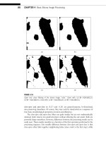
FIGURE 9.3
Example image randomly drawn from the Gaussian spectral model, with ␥ ϭ 2.0.
9.2 THE WAVELET MARGINAL MODEL
For decades, the inadequacy of the Gaussian model was apparent. But direct improve-
ment, through introduction of constraints on the Fourier phases, turned out to be
quite difficult. Relationships between phase components are not easily measured, in
part because of the difficulty of working with joint statistics of circular var iables, and in
part because the dependencies between phases of different frequencies do not seem to
be well captured by a model that is localized in frequency. A breakthrough occurred in
the 1980s, when a number of authors began to describe more direct indications of non-
Gaussian behaviors in images. Specifically, a multidimensional Gaussian statistical model
has the property that all conditional or marginal densities must also be Gaussian. But
these authors noted that histograms of bandpass-filtered natural images were highly non-
Gaussian [8, 14–17]. Specifically, their marginals tend to be much more sharply peaked
at zero, with more extensive tails, when compared with a Gaussian of the same variance.
As an example, Fig. 9.4 shows histograms of three images, filtered with a Gabor function

(a Gaussian-windowed sinuosoidal grating). The intuitive reason for this behavior is that
images typically contain smooth regions, punctuated by localized“features”such as lines,
edges, or corners. The smooth regions lead to small filter responses that genera te the
sharp peak at zero, and the localized features produce large-amplitude responses that
generate the extensive tails.
This basic behavior holds for essentially any zero-mean local filter, whether it i s
nondirectional (center-surround), or oriented, but some filters lead to responses that are
212 CHAPTER 9 Capturing Visual Image Properties with Probabilistic Models
Coefficient value
log (Porobability)
p 5 0.46
DH/H 5 0.0031
Coefficient value
log (Probability)
p 5 0.48
DH/H 5 0.0014
Coefficient value
log (Probability)
p 5 0.58
DH/H 5 0.0011
Coefficient value
log (Probability)
p 5 0.59
DH/H 5 0.0012
FIGURE 9.4
Log histograms of bandpass (Gabor) filter responses for four example images (see Fig. 9.1 for
image description). For each histogram, tails are truncated so as to show 99.8% of the distribution.
Also shown (dashed lines) are fitted generalized Gaussian densities, as specified by Eq. (9.3).
Text indicates the maximum-likelihood value of p of the fitted model density, and the relative
entropy (Kullback-Leibler divergence) of the model and histogram, as a fraction of the total

entropy of the histogram.
more non-Gaussian than others. By the mid-1990s, a number of authors had developed
methods of optimizing a basis of filters in order to maximize the non-Gaussianity of
the responses [e.g., 18, 19]. Often these methods operate by optimizing a higher-order
statistic such as kurtosis (the fourth moment divided by the squared variance). The
resulting basis sets contain oriented filters of different sizes with frequency bandwidths
of roughly one octave. Figure 9.5 shows an example basis set, obtained by optimiz-
ing kurtosis of the marginal responses to an ensemble of 12 ϫ 12 pixel blocks drawn
from a large ensemble of natural images. In parallel with these statistical developments,
authors from a variety of communities were developing multiscale orthonormal bases
for signal and image analysis, now generically known as “wavelets” (see Chapter 6 in this
Guide). These provide a good approximation to optimized bases such as that shown in
Fig. 9.5.
Once we have transformed the image to a multiscale representation, what statistical
model can we use to characterize the coefficients? The statistical motivation for the
choice of basis came from the shape of the marginals, and thus it would seem natural to
assume thatthe coefficients within asubband are independent and identicallydistributed.
With this assumption, the model is completely determined by the marginal statistics of
the coefficients, which can be examined empir ically as in the examples of Fig. 9.4.For
natural images, these histograms are surprisingly well described by a two-parameter
9.2 The Wavelet Marginal Model 213
FIGURE 9.5
Example basis functions derived by optimizing a marginal kurtosis criterion [see 22].
generalized Gaussian (also known as a stretched,orgeneralized exponential) distribution
[e.g., 16, 20, 21]:
P
c
(c;s,p) ϭ
exp(Ϫ|c/s|
p

)
Z(s,p)
, (9.3)
where the normalization constant is Z(s,p) ϭ 2
s
p
⌫

1
p

. An exponent of p ϭ 2corre-
sponds to a Gaussian density, and p ϭ 1 corresponds to the Laplacian density. In general,
smaller values of p lead to a density that is both more concentrated at zero and has
more expansive tails. Each of the histograms in Fig. 9.4 is plotted with a dashed curve
corresponding to the best fitting instance of this density function, with the parame-
ters {s,p} estimated by maximizing the probability of the data under the model. The
density model fits the histograms remarkably well, as indicated numerically by the rel-
ative entropy measures given below each plot. We have observed that values of the
exponent p t ypically lie in the range [0.4,0.8]. The factor s varies monotonically with
the scale of the basis functions, with correspondingly higher variance for coarser-scale
components.
This wavelet marginal model is significantly more powerful thanthe classicalGaussian
(spectral) model. For example, when applied to the problem of compression, the entropy
of the distributions described above is significantly less than that of a Gaussian with the
same variance, and this leads directly to gains in coding efficiency. In denoising, the use
of this model as a prior density for images yields to significant improvements over the
Gaussian model [e.g., 20, 21, 23–25]. Consider again the problem of removing additive
Gaussian white noise from an image. If the wavelet transform is orthogonal, then the
214 CHAPTER 9 Capturing Visual Image Properties with Probabilistic Models

noise remains white in the wavelet domain. The degradation process may be described
in the wavelet domain as:
P(d|c) ϰ ex p(Ϫ(d Ϫ c)
2
/2␴
2
n
),
where d is a wavelet coefficient of the observed (noisy) image, c is the corresponding
wavelet coefficient of the original (clean) image, and ␴
2
n
is the variance of the noise.
Again, using Bayes’ rule, we can reverse the conditioning:
P(c|d) ϰ ex p(Ϫ(d Ϫ c)
2
/2␴
2
n
) ·P(c),
where the prior on c is given by Eq. (9.3). Here, the MAP and BLS solutions cannot, in
general, be written in closed form, and they are unlikely to be the same. But numerical
solutions are fairly easy to compute, resulting in nonlinear estimators, in which small-
amplitude coefficients are suppressed and large-amplitude coefficients preserved. These
estimates show substantial improvement over the linear estimates associated with the
Gaussian model of the previous section.
Despite these successes, it is again easy to see that important attributes of images are
not capturedby wavelet marginal models.When thewavelet transform is orthonormal,we
can easily draw statistical samples from the model. Figure 9.6 shows the result of drawing
the coefficients of a wavelet representation independently from generalized Gaussian

densities. The density parameters for each subband were chosen as those that best fit an
example photographic image. Although it has more structure than an image of white
noise, and perhaps more than the image drawn from the spect ral model (Fig. 9.3), the
result still does not look very much like a photographic image!
FIGURE 9.6
A sample image drawn from the wavelet marginal model, with subband density parameters
chosen to fit the image of Fig. 9.7.
9.3 Wavelet Local Contextual Models 215
The wavelet marginal model may be improved by extending it to an overcomplete
wavelet basis. In particular, Zhu et al. have shown that large numbers of marginals
are sufficient to uniquely constrain a high-dimensional probability density [26] (this
is a variant of the Fourier projection-slice theorem used for tomographic reconstruc-
tion). Marginal models have been shown to produce better denoising results when the
multiscale representation is overcomplete [20, 27–30]. Similar benefits have been
obtained for texture representation and synthesis [26, 31]. The drawback of these models
is that the joint statistical properties are defined implicitly through the marginal statistics.
They are thus difficultto study directly,or to utilize in deriving optimalsolutions forimage
processing applications. In the next section, we consider the more direct development of
joint statistical descriptions.
9.3 WAVELET LOCAL CONTEXTUAL MODELS
The primary reason for the poor appearance of the image in Fig. 9.6 is that the coefficients
of the wavelet transform are not independent. Empirically, the coefficients of orthonor-
mal wavelet decompositions of visual images are found to bemoderately well decorrelated
(i.e., their covariance is near zero). But this is only a statement about their second-order
dependence, and one can easily see that there are important higher order dependencies.
Figure 9.7 shows the amplitudes (absolute values) of coefficients in a four-level separa-
ble orthonormal wavelet decomposition. First, we can see that individual subbands are
not homogeneous: Some regions have large-amplitude coefficients, while other regions
are relatively low in amplitude. The variability of the local amplitude is characteristic
of most photographic images: the large-magnitude coefficients tend to occur near each

other within subbands, and also occur at the same relative spatial locations in subbands
at adjacent scales and orientations.
The intuitive reason for the clustering of large-amplitude coefficients is that typical
localized and isolated image features are represented in the wavelet domain via the super-
position of a group of basis functions at different positions, orientations, and scales. The
signs and relative magnitudes of the coefficients associated with these basis functions
will depend on the precise location, orientation, and scale of the underlying feature. The
magnitudes will also scale with the contrast of the structure. Thus, measurement of a
large coefficient at one scale means that large coefficients at adjacent scales are more
likely.
This clustering property was exploited in a heuristic but highly effective manner in
the Embedded Zerotree Wavelet (EZW) image coder [32], and has been used in some
fashion in nearly all image compression systems since. A more explicit description had
been first developed for denoising, when Lee [33] suggested a two-step procedure, in
which the local signal variance is first estimated from a neighborhood of observed pixels,
after which the pixels in the neighborhood are denoised using a standard linear least
squares method. Although it was done in the pixel domain, this chapter introduced the
idea that variance is a local property that should be estimated adaptively, as compared
216 CHAPTER 9 Capturing Visual Image Properties with Probabilistic Models
FIGURE 9.7
Amplitudes of multiscale wavelet coefficients for an image of Albert Einstein. Each subimage
shows coefficient amplitudes of a subband obtained by convolution with a filter of a different
scale and orientation, and subsampled by an appropriate factor. Coefficients that are spatially
near each other within a band tend to have similar amplitudes. In addition, coefficients at different
orientations or scales but in nearby (relative) spatial positions tend to have similar amplitudes.
with the classical Gaussian model in which one assumes a fixed global variance. It was
not until the 1990s that a number of authors began to apply this concept to denoising in
the wavelet domain, estimating the variance of clusters of wavelet coefficients at nearby
positions, scales, and/or orientations, and then using these estimated variances in order
to denoise the cluster [20, 34–39].

The locally-adaptive variance principle is powerful, but does not constitute a full
probability model. As in the previous sections, we can develop a more explicit model by
directly examining the statistics of the coefficients. The top row of Fig. 9.8 shows joint
histograms of several different pairs of wavelet coefficients. As with the marginals, we
assume homogeneity in order to consider the joint histogram of this pair of coefficients,
gathered over the spatial extent of the image, as representative of the underlying density.
Coefficients that come from adjacent basis functions are seen to produce contours that
are nearly circular, whereas the others are clearly extended along the axes.
The joint histograms shown in the first row of Fig. 9.8 do not make explicit the issue
of whether the coefficients are independent. In order to make this more explicit, the
bottom row shows conditional histograms of the same data. Let x
2
correspond to the
9.3 Wavelet Local Contextual Models 217
Adjacent Near Far
2100 0 100
2150
2100
250
0
50
100
150
2100 0 100
2150
2100
250
0
50
100

150
2100 0 100
2150
2100
250
0
50
100
150
Other scale
Other ori
2500 0 500
2150
2100
250
0
50
100
150
2100 0 100
2150
2100
250
0
50
100
150
2100 0 100
2150
2100

250
0
50
100
150
2100 0 100
2150
2100
250
0
50
100
150
2100 0 100
2150
2100
250
0
50
100
150
2500 0 500
2150
2100
250
0
50
100
150
2100 0 100

2150
2100
250
0
50
100
150
FIGURE 9.8
Empirical joint distributions of wavelet coefficients associated with different pairs of basis func-
tions, for a single image of a New York City street scene (see Fig. 9.1 for image description).
The top row shows joint distributions as contour plots, with lines drawn at equal intervals of
log probability. The three leftmost examples correspond to pairs of basis functions at the same
scale and orientation, but separated by different spatial offsets. The next corresponds to a pair
at adjacent scales (but the same orientation, and nearly the same position), and the rightmost
corresponds to a pair at orthogonal orientations (but the same scale and nearly the same posi-
tion). The bottom row shows corresponding conditional distributions: brightness corresponds to
frequency of occurance, except that each column has been independently rescaled to fill the
full range of intensities.
density coefficient (vertical axis), and x
1
the conditioning coefficient (horizontal axis).
The histograms illustrate several important aspects of the relationship between the two
coefficients. First, the expected value of x
2
is approximately zero for all values of x
1
,
indicating that they are nearly decorrelated (to second order). Second, the variance of
the conditional histogram of x
2

clearly depends on the value of x
1
, and the strength of
this dependency depends on the particular pair of coefficients being considered. Thus,
although x
2
and x
1
are uncorrelated, they still exhibit statistical dependence!
The form of the histograms shown in Fig. 9.8 is surprisingly robust across a wide
range of images. Furthermore, the qualitative form of these statistical relationships also
holds for pairs of coefficients at adjacent spatial locations and adjacent orientations. As
one considers coefficients that are more distant (either in spatial position or in scale), the
dependency becomes weaker,suggesting that aMarkov assumption might be appropriate.
Essentially all of the statistical properties we have described thus far—the circular (or
elliptical) contours, the dependency between local coefficient amplitudes, as well as the
heavy-tailed marginals—can be modeled using a random field with a spatially fluctuat-
ing variance. These kinds of models have been found useful in the speech-processing
community [40]. A related set of models, known as autoregressive conditional het-
eroskedastic (ARCH) models [e.g., 41], have proven useful for many real signals that
suffer from abrupt fluctuations, followed by relative “calm” periods (stock mar ket prices,
for example). Finally, physicists studying properties of turbulence have noted similar
behaviors [e.g., 42].
218 CHAPTER 9 Capturing Visual Image Properties with Probabilistic Models
An example of a local density with fluctuating variance, one that has found particular
use in modeling local clusters (neighborhoods) of multiscale image coefficients, is the
product of a Gaussian vector and a hidden scalar multiplier. More formally, this model,
known as a Gaussian scale mixture [43] (GSM), expresses a random vector x as the
product of a zero-mean Gaussian vector u and an independent positive scalar r andom
variable

√
z:
x ∼
√
z u, (9.4)
where ∼indicates equality in distribution. The variable z is known as the multiplier .The
vector x is thus an infinite mixture of Gaussian vectors, whose density is determined by
the covariance matrix C
u
of v ector u and the mixing density, p
z
(z):
p
x
(x) ϭ

p(x|z) p
z
(z)dz
ϭ

exp

Ϫx
T
(zC
u
)
Ϫ1
x/2


(2␲)
N /2
|zC
u
|
1/2
p
z
(z)dz, (9.5)
where N is the dimensionalit y of x and u (in our case, the size of the neighborhood).
Notice thatsince thelevel surfaces (contours of constant probability) for P
u
(u) are ellipses
determined by the covariance matrix C
u
, and the density of x is constructed as a mixture
of scaled versions of the density of u, then P
x
(x) will also exhibit the same elliptical level
surfaces. In particular, if u is spherically symmetric (C
u
is a multiple of the identity),
then x will also be spherically symmetric. Figure 9.9 demonst rates that this model can
capture the strongly kurtotic behavior of the marginal densities of natural image wavelet
coefficients, as well as the correlation in their local amplitudes.
A number of recent image models describe the wavelet coefficients within each local
neighborhood using a Gaussian mixture model [e.g., 37, 38, 44–48]. Sampling from
these models is difficult, since the local description is typically used for overlapping
neighborhoods, and thus one cannot simply draw independent samples from the model

(see [48] for an example). The underlying Gaussian structure of the model allows it to
be adapted for problems such as denoising. The resulting estimator is more complex
than that described for the Gaussian or wavelet marginal models, but performance is
significantly better.
As with the models of the previous two sections, there are indications that the GSM
model is insufficientto fully capture the structure of typical visual images.Todemonstrate
this, we note that normalizing each coefficient by (the square root of) its estimated
variance should produce a field of Gaussian white noise [4, 49]. Figure 9.10 illustrates
this process, showing an example wavelet subband, the estimated variance field, and the
normalized coefficients. But note that there are two important types of structure that
remain. First, although the normalized coefficients are certainly closer to a homogeneous
field, the signs of the coefficients still exhibit important structure. Second, the variance
field itself is far from homogeneous, with most of the significant values concentrated on
one-dimensional contours. Some of these attributes can be captured by measuring joint
statistics of phase and amplitude, as has been demonstrated in texture modeling [50].
9.3 Wavelet Local Contextual Models 219
Ϫ
50
0
50
10
0
10
5
10
0
10
5
Ϫ
50

0
50
(a) Observed (b) Simulated
(c) Observed
(d) Simulated
FIGURE 9.9
Comparison of statistics of coefficients from an example image subband (left panels) with those
generated by simulation of a local GSM model (right panels). Model parameters (covariance
matrix and the multiplier prior density) are estimated by maximizing the likelihood of the subband
coefficients (see [47]). (a,b) Log of marginal histograms. (c,d) Conditional histograms of two
spatially adjacent coefficients. Pixel intensity corresponds to frequency of occurance, except
that each column has been independently rescaled to fill the full range of intensities.
Original coefficients Estimated Œ„z field Normalized coefficients
FIGURE 9.10
Example wavelet subband, square root of the variance field, and normalized subband.
220 CHAPTER 9 Capturing Visual Image Properties with Probabilistic Models
9.4 DISCUSSION
After nearly 50 years of Fourier/Gaussian modeling, the late 1980s and 1990s saw sud-
den and remarkable shift in viewpoint, arising from the confluence of (a) multiscale
image decompositions, (b) non-Gaussian statistical observations and descriptions, and
(c) locally-adaptive statistical models based on fluctuating variance. The improvements
in image processing applications arising from these ideas have been steady and substan-
tial. But the complete synthesis of these ideas and development of further refinements
are still under way.
Variants of the contextual models described in the previous section seem to represent
the current state-of-the-art,both interms of characterizing the density of coefficients,and
in terms of the quality of results in image processing applications. There are several issues
that seem to be of primary importance in trying to extend such models. First,a number of
authors are developing models that can capture the regularities in the local variance, such
as spatialrandom fields [48, 51–53], and multiscale tree-structured models[38, 45]. Much

of the structure in the var iance field may be attributed to discontinuous features such
as edges, lines, or corners. There is substantial literature in computer vision describing
such structures, but it has proven difficult to establish models that are both explicit about
these features and yet flexible. Finally, there have been several recent studies investigat-
ing geometric regularities that arise from the continuity of contours and boundaries
[54–58]. These and other image regularities will surely be incorporated into future
statistical models, leading to further improvements in image processing applications.
REFERENCES
[1] G. Buchsbaum and A. Gottschalk. Trichromacy, opponent color coding, and optimum colour
information transmission in the retina. Proc. R. Soc. Lond., B, Biol. Sci., 220:89–113, 1983.
[2] D. L. Ruderman, T. W. Cronin, and C C. Chiao. Statistics of cone responses to natural images:
implications for visual coding. J. Opt. Soc. Am. A, 15(8):2036–2045, 1998.
[3] D. W. Dong and J. J. Atick. Statistics of natural time-varying images. Network Comp. Neural,
6:345–358, 1995.
[4] D. L. Ruderman. The statistics of natural images. Network Comp. Neural, 5:517–548, 1996.
[5] E. T. Jaynes. Where do we stand on maximum entropy? In R. D. Levine and M. Tribus, editors, The
Maximal Entropy Formalism. MIT Press, Cambridge, MA, 1978.
[6] G. Strang. Linear Algebra and its Applications. Academic Press, Orlando, FL, 1980.
[7] N. G. Deriugin. The power spectrum and the correlation function of the television signal.
Telecomm., 1(7):1–12, 1956.
[8] D. J. Field. Relations between the statistics of natural images and the response properties of cortical
cells. J. Opt. Soc. Am. A, 4(12):2379–2394, 1987.
[9] D. J. Tolhurst, Y. Tadmor, and T. Chao. Amplitude spect ra of natural images. Ophthalmic Physiol.
Opt., 12:229–232, 1992.
References 221
[10] D. L. Ruderman and W. Bialek. Statistics of natural images: scaling in the woods. Phys.Rev.Lett.,
73(6):814–817, 1994.
[11] A. van der Schaaf and J. H. van Hateren. Modelling the power spectra of natural images: statistics
and information. Vision Res., 28(17):2759–2770, 1996.
[12] A. Turiel and N. Parga. The multi-fractal structure of contrast changes in natural images: from

sharp edges to textures. Neural. Comput., 12:763–793, 2000.
[13] A. V. Oppenheim and J. S. Lim. The importance of phase in signals. Proc. IEEE, 69:529–541, 1981.
[14] P. J. Burt and E. H. Adelson. The Laplacian pyramid as a compact image code. IEEE Trans. Comm.,
COM-31(4):532–540, 1983.
[15] J. G. Daugman. Complete discrete 2-D Gabor transforms by neural networks for image analysis
and compression. IEEE Trans. Acoust., 36(7):1169–1179, 1988.
[16] S. G. Mallat. A theory for multiresolution signal decomposition: the wavelet representation. IEEE
Trans. Pattern Anal. Mach. Intell., 11:674–693, 1989.
[17] C. Zetzsche and E. Barth. Fundamental limits of linear filters in the visual processing of two-
dimensional signals. Vision Res., 30:1111–1117, 1990.
[18] B. A. Olshausen and D. J. Field. Sparse coding with an overcomplete basis set: a strategy employed
by V1? Vision Res., 37:3311–3325, 1997.
[19] A. J. Bell and T. J. Sejnowski. The independent components of natural scenes are edge filters. Vision
Res., 37(23):3327–3338, 1997.
[20] E. P. Simoncelli. Bayesian denoising of visual images in the wavelet domain. In P. Müller and
B. Vidakovic, editors, Bayesian Inference in Wavelet Based Models, Vol. 141, 291–308. Springer-
Verlag, New York, Lecture Notes in Statistics, 1999.
[21] P. Moulin and J. Liu. Analysis of multiresolution image denoising schemes using a generalized
Gaussian and complexity priors. IEEE Trans. Inf. Theory, 45:909–919, 1999.
[22] B. A. Olshausen and D. J. Field. Emergence of simple-cell receptive field properties by learning a
sparse code for natural images. Nature, 381:607–609, 1996.
[23] E. P. Simoncelli and E. H. Adelson. Noise removal v ia Bayesian wavelet coring. In Proc. 3rd IEEE
Int. Conf. on Image Process., Vol. I, 379–382, IEEE Signal Processing Society, Lausanne, September
16–19, 1996.
[24] H. A. Chipman, E. D. Kolaczyk, and R. M. McCulloch. Adaptive Bayesian wavelet shrinkage. JAm.
Stat. Assoc., 92(440):1413–1421, 1997.
[25] F. Abramovich, T. Sapatinas, and B. W. Silverman. Wavelet thresholding via a Bayesian approach.
J. Roy. Stat. Soc. B, 60:725–749, 1998.
[26] S. C. Zhu, Y. N. Wu, and D. Mumford. FRAME: filters, random fields and maximum entropy –
towards a unified theory for texture modeling. Int. J. Comput. Vis., 27(2):1–20, 1998.

[27] R. R. Coifman and D. L. Donoho. Translationinvariant de-noising. In A. Antoniadis and G.
Oppenheim, editors, Wavelets and Statistics, Springer-Verlag, Lecture notes, San Diego, CA, 1995.
[28] F. Abramovich,T. Sapatinas, and B. W. Silverman. Stochastic expansions in anovercomplete wavelet
dictionary. Probab. Theory Rel., 117:133–144, 2000.
[29] X. Li and M. T. Orchard. Spatially adaptive image denoising under overcomplete expansion. In
IEEE Int. Conf. on Image Process., Vancouver, September 2000.
[30] M. Raphan and E. P. Simoncelli. Optimal denoising in redundant representations. IEEE Trans.
Image Process., 17(8):1342–1352, 2008.
222 CHAPTER 9 Capturing Visual Image Properties with Probabilistic Models
[31] D. Heeger and J. Bergen. Pyramid-based texture analysis/synthesis. In Proc. ACM SIGGRAPH,
229–238. Association for Computing Machinery, August 1995.
[32] J. Shapiro. Embedded image coding using zerotrees of wavelet coefficients. IEEE Trans. Signal
Process., 41(12):3445–3462, 1993.
[33] J. S. Lee. Digital image enhancement and noise filtering by use of local statistics. IEEE T. Pattern
Anal., PAMI-2:165–168, 1980.
[34] M. Malfait and D. Roose. Wavelet-based image denoising using a Markov random field a priori
model. IEEE Trans. Image Process., 6:549–565, 1997.
[35] E. P. Simoncelli. Statistical models for images: compression, restoration and synthesis. In Proc. 31st
Asilomar Conf. on Signals, Systems and Computers, Vol. 1, 673–678, IEEE Computer Society, Pacific
Grove, CA, November 2–5, 1997.
[36] S. G. Chang, B. Yu, and M. Vetterli. Spatially adaptive wavelet thresholding with context modeling
for image denoising. In Fifth IEEE Int. Conf. on Image Process., IEEE Computer Society, Chicago,
October 1998.
[37] M. K. Mihçak, I. Kozintsev, K. Ramchandran, and P. Moulin. Low-complexity image denoising
based on statistical modeling of wavelet coefficients. IEEE Signal Process. Lett., 6(12):300–303,
1999.
[38] M. J. Wainwright, E. P. Simoncelli, and A. S. Willsky. Random cascadeson wavelet trees and theiruse
in modeling and analyzing natural imagery. Appl. Comput. Harmonic Anal., 11(1):89–123, 2001.
[39] F. Abramovich, T. Besbeas, and T. Sapatinas. Empirical Bayes approach to block wavelet function
estimation. Comput. Stat. Data. Anal., 39:435–451, 2002.

[40] H. Brehm and W. Stammler. Description and generation of spherically invariant speech-model
signals. Signal Processing, 12:119–141, 1987.
[41] T. Bollersley, K. Engle, and D. Nelson. ARCH models. In B. Engle and D. McFadden, editors,
Handbook of Econometrics IV, North Holland, Amsterdam, 1994.
[42] A. Turiel, G. Mato, N. Parga, and J. P. Nadal. The self-similarity properties of natural images
resemble those of turbulent flows. Phys.Rev.Lett., 80:1098–1101, 1998.
[43] D. Andrews and C. Mallows. Scale mixtures of normal distributions. J. Roy. Stat. Soc., 36:99–102,
1974.
[44] M. S. Crouse, R. D. Nowak, and R. G. Baraniuk. Wavelet-based statistical signal processing using
hidden Markov models. IEEE Trans. Signal Process., 46:886–902, 1998.
[45] J. Romberg, H. Choi, and R. Baraniuk. Bayesian wavelet domain image modeling using hidden
Markov trees. In Proc. IEEE Int. Conf. on Image Process., Kobe, Japan, October 1999.
[46] S. M. LoPresto, K. Ramchandran, and M. T. Orchard. Wavelet image coding based on a new
generalized Gaussian mixture model. In Data Compression Conf., Snowbird, Utah, March 1997.
[47] J. Portilla, V. Strela, M. J. Wainwright, and E. P. Simoncelli. Image denoising using a scale mixture
of Gaussians in the wavelet domain. IEEE Trans. Image Process., 12(11):1338–1351, 2003.
[48] S. Lyu and E. P. Simoncelli. Modeling multiscale subbands of photographic images with fields of
Gaussian scale mixtures. IEEE Trans. Pattern Anal. Mach. Intell., 2008. Accepted for publication,
4/08.
[49] M. J. Wainwright and E. P. Simoncelli. Scale mixtures of Gaussians and the statistics of natural
images. In S. A. Solla, T. K. Leen, and K R. Müller,editors,Advances in Neural Information Processing
Systems (NIPS*99), Vol. 12, 855–861. MIT Press, Cambridge, MA, 2000.
References 223
[50] J. Portilla and E. P. Simoncelli. A parametric texture model based on joint statistics of complex
wavelet coefficients. Int. J. Comput. Vis., 40(1):49–71, 2000.
[51] A. Hyvärinen and P. Hoyer. Emergence of topography and complex cell properties from natural
images using extensions of ICA. In S. A. Solla, T. K. Leen, and K R. Müller, editors, Advances in
Neural Information Processing Systems, Vol. 12, 827–833. MIT Press, Cambridge, MA, 2000.
[52] Y. Karklin and M. S. Lewicki. Learning higher-order structures in natural images. Network, 14:483–
499, 2003.

[53] A. Hyvärinen, J. Hurri, and J. Väyrynen. Bubbles: a unifying framework for low-level statistical
properties of natural image sequences. J. Opt. Soc. Am. A, 20(7):2003.
[54] M. Sigman, G. A. Cecchi, C. D. Gilbert, and M. O. Magnasco. On a common circle: natural scenes
and Gestalt rules. Proc. Natl. Acad. Sci., 98(4):1935–1940, 2001.
[55] J. H. Elder and R. M. Goldberg. Ecological statistics of gestalt laws for the perceptual organization
of contours. J. Vis., 2(4):324–353, 2002. DOI 10:1167/2.4.5.
[56] W. S. Geisler, J. S. Perry, B. J. Super, and D. P. Gallogly. Edge co-occurance in natural images predicts
contour grouping performance. Vision Res., 41(6):711–724, 2001.
[57] P. Hoyer and A. Hyvärinen. A multi-layer sparse coding network learns contour coding from natural
images. Vision Res., 42(12):1593–1605, 2002.
[58] S C. Zhu. Statistical modeling and conceptualization of visual patterns. IEEE Trans. Pattern Anal.
Mach. Intell., 25(6):691–712, 2003.
CHAPTER
10
Basic Linear Filtering with
Application to Image
Enhancement
Alan C. Bovik
1
and Scott T. Acton
2
1
The University of Texas at Austin;
2
University of Virginia
10.1 INTRODUCTION
Linear system theory and linear filtering play a central role in digital image processing.
Many potent techniques for modifying, improving, or representing digital visual data
are expressed in terms of linear systems concepts. Linear filters are used for generic
tasks such as image/video contrast improvement, denoising, and sharpening, as well

as for more object- or feature-specific tasks such as target matching and feature
enhancement.
Much of this Guide deals with the application of linear filters to image and video
enhancement, restoration, reconstruction, detection, segmentation, compression, and
transmission. The goal of this chapter is to introduce some of the basic supporting
ideas of linear systems theory as they apply to digital image filtering, and to out-
line some of the applications. Special emphasis is given to the topic of linear image
enhancement.
We will require some basic concepts and definitions in order to proceed. The basic
2D discrete-space signal is the 2D impulse function, defined by
␦(m Ϫ p, n Ϫ q) ϭ

1; m ϭ p and n ϭ q
0; else
. (10.1)
Thus, (10.1) takes unit value at coordinate (p, q) and is everywhere else zero. The function
in (10.1) is often termed the Kronecker delta function or the unit sample sequence [1].It
plays the same role and has the same significance as the so-called Dirac delta function of
continuous system theory. Specifically, the response of linear systems to (10.1) will be
used to characterize the general responses of such systems.
225
226 CHAPTER 10 Basic Linear Filtering with Application to Image Enhancement
Any discrete-space image f may be expressed in terms of the impulse function (10.1):
f (m, n) ϭ
ϱ

pϭϪϱ
ϱ

qϭϪϱ

f (m Ϫ p,n Ϫ q) ␦(p,q) ϭ
ϱ

pϭϪϱ
ϱ

qϭϪϱ
f (p,q) ␦(m Ϫ p,n Ϫ q). (10.2)
The expression (10.2),called the sifting property, has two meaningful interpretations here.
First, any discrete-space image can be written as a sum of weighted, shifted unit impulses.
Each weighted impulse comprises one of the pixels of the image. Second, the sum in
(10.2) is in fact a discrete-space linear convolution. As is apparent, the linear convolution
of any image f w ith the impulse function ␦ returns the function unchanged.
The impulse function effectively describes certain systems known as linear space-
invariant (LSI ) systems. We explain these terms next.
A2DsystemL is a process of image transformation, as shown in Fig. 10.1:
We can write
g (m,n) ϭ L[f (m, n)]. (10.3)
The system L is linear if and only if for any two constants a, b and for any f
1
(m,n),
f
2
(m,n) such that
g
1
(m,n) ϭ L[f
1
(m,n)] and g
2

(m,n) ϭ L[f
2
(m,n)], (10.4)
then
a ·g
1
(m,n) ϩ b ·g
2
(m,n) ϭ L[a ·f
1
(m,n) ϩ b ·f
2
(m,n)] (10.5)
for every (m, n). This is often called the superposition property of linear systems.
The system L is shift-invariant if for every f(m, n) such that (10.3) holds, then also
g (m Ϫ p,n Ϫ q) ϭ L[f (m Ϫ p, n Ϫ q)] (10.6)
for any (p, q). Thus, a spatial shift in the input to L produces no change in the output,
except for an identical shift.
The rest of this chapter will be devoted to studying systems that are linear and shift-
invariant (LSI). In this and other chapters, it will b e found that LSI systems can be
used for many powerful image and video processing tasks. In yet other chapters, nonlin-
earity and/or space-variance will be shown to afford certain advantages, particularly in
surmounting the inherent limitations of LSI systems.
f
(m, n)
g(m, n)
L
FIGURE 10.1
Two-dimensional input-output system.
10.2 Impulse Response, Linear Convolution, and Frequency Response 227

10.2 IMPULSE RESPONSE, LINEAR CONVOLUTION,
AND FREQUENCY RESPONSE
The unit impulse response of a 2D input-output system L is
L [␦(m Ϫ p,n Ϫ q)] ϭ h(m,n ; p, q). (10.7)
This is the response of system L, at spatial position (m,n), to an impulse located at
spatial position (p,q). Generally, the impulse response is a function of these four spatial
variables. However, if the system L is space-invariant, then if
L [␦( m,n)] ϭ h(m,n) (10.8)
is the response to an impulse applied at the spatial origin, then also
L [␦( m Ϫ p, n Ϫ q)] ϭ h(m Ϫ p, n Ϫ q), (10.9)
which means that the response to an impulse applied at any spatial position can be found
from the impulse response (10.8).
As already mentioned, the discrete-space impulse response h(m, n) completely char-
acterizes the input-output response of LSI input-output systems. This means that if the
impulse response is known, then an expression can be found for the response to any
input. The form of the expression is 2D discrete-space linear convolution.
Consider the generic system L shown in Fig. 10.1, with input f (m, n) and output
g (m, n). Assume that the response is due to the input f only (the system would be at rest
without the input). Then from (10.2):
g (m,n) ϭ L[f (m, n)] ϭ L
⎡
⎣
ϱ

pϭϪϱ
ϱ

qϭϪϱ
f (p,q)␦(m Ϫ p,n Ϫ q)
⎤

⎦
. (10.10)
If the system is known to be linear, then
g (m,n) ϭ
ϱ

pϭϪϱ
ϱ

qϭϪϱ
f (p,q)L[␦(m Ϫ p,n Ϫ q)] (10.11)
ϭ
ϱ

pϭϪϱ
ϱ

qϭϪϱ
f (p,q)h(m, n;p,q), (10.12)
which is all that generally can be said without further knowledge of the system and the
input. If it is known that the system is space-invariant (hence LSI), then (10.12) becomes
g (m,n) ϭ
ϱ

pϭϪϱ
ϱ

qϭϪϱ
f (p,q)h(m Ϫ p, n Ϫ q) (10.13)
ϭ f (m, n)

∗
h(m, n), (10.14)
which is the 2D discrete-space linear convolution of input f with impulse response h.
The linearconvolution expresses theoutput of awide variety of electrical andmechan-
ical systems. In continuous systems, the convolution is expressed as an integral. For
example, with lumped electrical circuits, the convolution integral is computed in terms
228 CHAPTER 10 Basic Linear Filtering with Application to Image Enhancement
of the passive circuit elements (resistors, inductors, capacitors). In optical systems, the
integral utilizes the point spread functions of the optics. The operations occur effectively
instantaneously, with the computational speed limited only by the speed of the electrons
or photons through the system elements.
However, in discrete signal and image processing systems, the discrete convolutions
are calculated sums of products. This convolution can be directly evaluated at each
coordinate (m,n) by a digital processor, or, as discussed in Chapter 5, it can be compu-
ted using the DFT using an FFT algorithm. Of course, if the exact linear convolution is
desired, this means that the involved functions must be appropriately zero-padded prior
to using the DFT, as discussed in Chapter 5. The DFT/FFT approach is usually, but not
always faster. If an image is being convolved with a very small spatial filter, then direct
computation of (10.14) can be faster.
Suppose that the input to a discrete LSI system with impulse response h(m,n) is a
complex exponential function:
f (m, n) ϭ e
2␲j(UmϩVn)
ϭ cos[2␲(Um ϩ Vn)]ϩ j sin[2␲(Um ϩ Vn)]. (10.15)
Then the system response is the linear convolution:
g (m,n) ϭ
ϱ

pϭϪϱ
ϱ


qϭϪ ϱ
h(p, q)f (m Ϫ p,n Ϫ q) ϭ
ϱ

pϭϪϱ
ϱ

qϭϪϱ
h(p, q)e
2␲j[U(mϪp)ϩV (nϪq)]
(10.16)
ϭ e
2␲j(UmϩVn)
ϱ

pϭϪϱ
ϱ

qϭϪϱ
h(p, q)e
Ϫ2␲j(UpϩVq)
, (10.17)
which is exactly the input f (m,n) ϭ e
2␲j(UmϩVn)
multiplied by a function of (U , V )
only:
H(U ,V ) ϭ
ϱ


pϭϪϱ
ϱ

qϭϪϱ
h(p, q)e
Ϫ2␲j(UpϩVq)
ϭ |H (U , V )|·e
j∠H(U ,V )
. (10.18)
The function H(U , V ), which is immediately identified as the discrete-space Fourier
transform (or DSFT, discussed extensively in Chapter 5) of the system impulse response,
is called the frequency response of the system.
From (10.17) it may be seen that the response to any complex exponential sinusoid
function, with frequencies (U, V ), is the same sinusoid, but with its amplitude scaled by
the system magnitude response


H(U, V )


evaluated at (U, V ) and with a shift equal to
the system phase response ∠H (U, V )at(U ,V ). The complex sinusoids are the unique
functions that have this invariance property in LSI systems.
As mentioned, the impulse response h(m, n) of a LSI system is sufficient to express
the response of the system to any input.
1
The frequency response H (U,V ) is uniquely
1
Strictly speaking, for any bounded input, and provided that the system is stable. In practical image
processing systems, the inputs are invariably bounded. Also, almost all image processing filters do not

involve feedback, and hence are naturally stable.
10.2 Impulse Response, Linear Convolution, and Frequency Response 229
obtainable from the impulse response (and v ice versa), and so contains sufficient
information to compute the response to any input that has a DSFT. In fact, the out-
put can be expressed in terms of the frequency response via G(U ,V )ϭF(U,V )H(U ,V )
and via the DFT/FFT with appropriate zero-padding. In fact, throughout this chapter
and elsewhere, it may be assumed that whenever a DFT is being used to compute linear
convolution, the appropriate zero-padding has been applied to avoid the wraparound
effect of the cyclic convolution.
Usually, linear image processing filters are characterized in terms of their frequency
responses, specifically by their spectrum shaping properties. Coarse descriptions that
apply to many 2D image processing filters include lowpass, bandpass,or highpass. In such
cases, the frequency response is primarily a function of radial frequency, and may even
be circularly symmetric, viz., a function of U
2
ϩ V
2
only. In other cases, the filter may
be strongly directional or oriented, with response strongly depending on the frequency
angle of the input. Of course, the terms lowpass, bandpass, highpass, and oriented are
only rough qualitative descriptions of a system frequency response. Each broad class of
filters has some generalized applications. For example, lowpass filters strongly attenuate
all but the “lower” radial image frequencies (as determined by some bandwidth or cutoff
frequency), and so are primarily smoothing filters. They are commonly used to reduce
high-frequency noise, or to eliminate all but coarse image features, or to reduce the
bandwidth of an image prior to transmission through a low-bandwidth communication
channel or before subsampling the image.
A (ra dial frequency) bandpass filter attenuates all but an intermediate range of “mid-
dle” radial frequencies. This is commonly used for the enhancement of certain image
features, such as edges (sudden transitions in intensity) or the ridges in a fingerprint.

A highpass filter attenuates all but the “higher” radial frequencies, or commonly, signifi-
cantly amplifies high frequencies without attenuating lower frequencies. This approach
is often used for correcting images that are blurred—see Chapter 14.
Oriented filters tend to be more specialized. Such filters attenuate frequencies falling
outside of a narrow range of orientations or amplify a narrow range of angular frequen-
cies. For example, it may be desirable to enhance vertical image features as a prelude to
detecting vertical structures, such as buildings.
Of course, filters may be a combination of types, such as bandpass and oriented. In
fact, such filters are the most common types of basis functions used in the powerful
wavelet image decompositions (Chapters 6, 11, 17, 18).
In the remainder of this chapter, we introduce the simple but important application
of linear filtering for linear image enhanceme nt, which specifically means attempting to
smooth image noise while not disturbing the original image structure.
2
2
The term “image enhancement” has been widely used in the past to describe any operation that
improves image quality by some criteria. However, in recent years, the meaning of the term has evolved
to denote image-preserving noise smoothing. This primarily serves to distinguish it from similar-
sounding terms, such as “image restoration” and “image reconstruction,” which also have taken specific
meanings.
230 CHAPTER 10 Basic Linear Filtering with Application to Image Enhancement
10.3 LINEAR IMAGE ENHANCEMENT
The term “enhancement” implies a process whereby the visual quality of the image is
improved. However, the term “image enhancement” has come to specifically mean a
process of smoothing irregularities or noise that has somehow corru pted the image,
while modifying the original image information as little as possible. The noise is usually
modeled as an additive noise or as a multiplicative noise. We will consider additive noise
now. As noted in Chapter 7, multiplicative noise, which is the other common type, can
be converted into additive noise in a homomorphic filtering approach.
Before considering methods for image enhancement, we will make a simple model

for additive noise. Chapter 7 of this Guide greatly elaborates image noise models, which
prove particularly useful for studying image enhancement filters that are nonlinear.
We will make the practical assumption that an observed noisy image is of finite
extent M ϫ N : f ϭ [f (m, n);0Յ m Յ M Ϫ 1, 0 Յ n Յ N Ϫ 1].Wemodelf asasum
of an original image o and a noise image q:
f ϭ o ϩ q, (10.19)
where n ϭ (m,n). The additive noise image q models an undesirable, unpredictable
corruption of o. The process q is called a 2D random process or a random field. Random
additive noise can occur as thermal circuit noise, communication channel noise, sensor
noise, and so on. Quite commonly, the noise is present in the image signal before it is
sampled, so the noise is also sampled coincident with the image.
In (10.19), both the original image and noise image are unknown. The goal of
enhancement is to recover an image g that resembles o as closely as possible by reducing q.
If there is an adequate model for the noise, then the problem of finding g can be posed as
an image estimation problem, where g is found as the solution to a statistical optimiza-
tion problem. Basic methods for image estimation are also discussed in Chapter 7, and
in some of the following chapters on image enhancement using nonlinear filters.
With the tools of Fourier analysis and linear convolution in hand, we will now outline
the basic approach of image enhancement by linear filtering. More often than not, the
detailed statistics of the noise process q are unknown. In such cases, a simple linear filter
approach can yield acceptable results, if the noise satisfies cer tain simple assumptions.
We will assume a zero-mean additive white noise model. The zero-mean model is used
in Chapter 3, in the context of frame averaging. The process q is zero-mean if the average
or sample mean of R arbitrary noise samples

1
R

R


rϭ1
q(m
r
,n
r
) → 0 (10.20)
as R grows large (provided that the noise process is mean-ergodic, which means that the
sample mean approaches the statistical mean for large samples).
The term white nois e is an idealized model for noise that has, on the average, a broad
spectrum. It is a simplified model for wideband noise . More precisely, if Q(U, V ) is the
DSFT of the noise process q, then Q is also a random process. It is called the energy
10.3 Linear Image Enhancement 231
spectrum of the random process q. If the noise process is white, then the average squared
magnitude of Q( U ,V ) takes constant over all frequencies in the range [Ϫ␲, ␲]. In the
ensemble sense, this means that the sample average of the magnitude spectra of R noise
images generated from the same source becomes constant for large R:

1
R

R

rϭ1
|Q
r
(U ,V )|→␩ (10.21)
for all (U , V ) as R grows large. The square ␩
2
of the constant level is called the noise power.
Since q has finite-extent M ϫ N ,ithasaDFT

˜
Q ϭ [
˜
Q(u, v) :0Յ u Յ M Ϫ 1,0 Յ v Յ
N Ϫ 1]. On average, the magnitude of the noise DFT
˜
Q will also be flat. Of course, it is
highly unlikely that a given noise DSFT or DFT will actually have a flat magnitude spec-
trum. However,it is an effective simplified model for unknown, unpredictable broadband
noise.
Images are also generally thought of as relatively broadband signals. Significant visual
information may reside at mid-to-high spatial frequencies,since visually significantimage
details such as edges, lines, and textures typically contain higher frequencies. However,
the magnitude spectrum of the image at higher image frequencies is usually relatively
low; most of the image power resides in the low frequencies contributed by the dominant
luminance effects. Nevertheless, the higher image frequencies are visually significant.
The basic approach to linear image enhancement is lowpass filtering. There are differ-
ent types of lowpass filters that can be used; several will be studied in the following. For
a given filter type, different degrees of smoothing can be obtained by adjusting the filter
bandwidth. A narrower bandwidth lowpass filter will reject more of the high-frequency
content of white or broadband noise, but it may also degrade the image content by
attenuating important high-frequency image details. This is a tradeoff that is difficult to
balance.
Next we describe and compare several smoothing lowpass filters that are commonly
used for linear image enhancement.
10.3.1 Moving Average Filter
The moving average filter can be described in several equivalent ways. First, using the
notion of window ing introduced in Chapter 4, the moving average can be defined as an
algebraic operation performed on local image neighborhoods according to a geometric
rule defined by the window. Given an image f to be filtered and a window B that collects

gray level pixels according to a geometric rule (defined by the window shape), then the
moving average-filtered image g is g iven by
g (n) ϭ AV E [Bf (n)], (10.22)
where the operation AVE computes the sample average of its. Thus, the local average is
computed over each local neighborhood of the image, producing a powerful smoothing
effect. The windows are usually selected to be symmetric, as with those used for binary
morphological image filtering (Chapter 4).
232 CHAPTER 10 Basic Linear Filtering with Application to Image Enhancement
Since the average is a linear operation, it is also true that
g (n) ϭ AV E [Bo(n)]ϩ AVE [Bq(n)]. (10.23)
Because the noise process q is assumed to be zero-mean in the sense of (10.20), then
the last term in (10.23) will tend to zero as the filter window is increased. Thus, the
moving average filter has the desirable effect of reducing zero-mean image noise toward
zero. However, the filter also effects the original image information. It is desirable that
AVE [Bo(n)]≈o(n) at each n, but this will not be the case everywhere in the image if the
filter window is too large. The moving average filter, which is lowpass, will blur the image,
especially as the window span is increased. Balancing this t radeoff is often a difficult task.
The moving average filter operation (10.22) is actually a linear convolution. In fact,
the impulse response of the filter is defined as having value 1/R over the span covered by
the window when centered at the spatial origin (0, 0), and zero elsewhere, where R is the
number of elements in the window.
For example, if the window is SQUARE [(2P ϩ 1)
2
], which is the most common
configuration (it is defined in Chapter 4), then the average filter impulse response is
given by
h(m, n) ϭ

1/
(

2P ϩ 1
)
2
; ϪP Յ m,n Յ P
0 ; else
. (10.24)
The frequency response of the moving average filter (10.24) is:
H(U ,V ) ϭ
sin
[
(
2P ϩ 1
)
␲U
]
(
2P ϩ 1
)
sin
(
␲U
)
·
sin
[
(
2P ϩ 1
)
␲V
]

(
2P ϩ 1
)
sin
(
␲V
)
. (10.25)
The half-peak bandwidth is often used for image processing filters. The half-peak (or
3 dB) cutoff frequencies occur on the locus of points (U, V )where|H (U ,V )| falls to
1/2. For the filter (10.25), this locus intersects the U -axis and V -axis at the cutoffs
U
half-peak
,V
half-peak
≈ 0.6/(2P ϩ 1) cycles/pixel.
As depicted in Fig. 10.2, the magnitude response |H (U ,V )| of the filter (10.25)
exhibits considerable sidelobes. In fact, the number of sidelobes in the range [0, ␲]is P.As
P is increased, the filter bandwidth naturally decreases (more high-frequency attenuation
or smoothing), but the overall sidelobe energy does not. The sidelobes are in fact a
significant drawback, since there is considerable noise leakage at high noise frequencies.
These residual noise frequencies remain to degrade the image. Nevertheless, the moving
average filter has been commonly used because of its genera l effectiveness in the sense of
(10.21) and because of its simplicity (ease of programming).
The moving average filter can be implemented either as a direct 2D convolution in
the space domain, or using DFTs to compute the linear convolution (see Chapter 5).
Since application of the moving average filter balances a tradeoff between noise
smoothing and image smoothing, the filter span is usually taken to be an intermedi-
ate value. For images of the most common sizes, e.g., 256 ϫ 256 or 512 ϫ 512, typical
(SQUARE) average filter sizes range from 3 ϫ 3to15ϫ 15. The upper end provides sig-

nificant (and probably excessive) smoothing, since 225 image samples are being averaged
10.3 Linear Image Enhancement 233
|H(U, 0)|
P5 1
P5 2
P 5 3
P 5 4
0
0.2
0.4
0.6
0.8
1
21/2 0.0 1/2
U
FIGURE 10.2
Plots of |H(U ,V )| given in (10.25) along V ϭ 0, for P ϭ 1,2,3, 4. As the filter span is increased,
the bandwidth decreases. The number of sidelobes in the range [0, ␲]isP.
to produce each new image value. Of course, if an image suffers from severe noise, then
a larger window might be used. A large window might also be acceptable if it is known
that the original image is very smooth everywhere.
Figure 10.3 depicts the application of the moving average filter to an image that has
had zero-mean white Gaussian noise added to it. In the current context, the distribution
(Gaussian) of the noise is not relevant, althoug h the meaning can be found in Chapter 7.
The original image is included for comparison. The image was filtered with SQUARE-
shaped moving average filters of window sizes 5 ϫ 5 and 9 ϫ 9, producing images with
significantly different appearances from each other as well as the noisy image. With
the 5 ϫ 5 filter, the noise is inadequately smoothed, yet the image has been blurred
noticeably. The result of the 9 ϫ 9 moving average filter is much smoother, although the
noise influence is still visible, with some higher noise frequency components managing

to leak through the filter, resulting in a mottled appearance.
10.3.2 Ideal Lowpass Filter
As an alternative to the average filter, a filter may be designed explicitly with no side-
lobes by forcing the frequency response to be zero outside of a given radial cutoff
frequency ⍀
c
:
H(U ,V ) ϭ

1;
√
U
2
ϩ V
2
Յ⍀
c
0; else
(10.26)
234 CHAPTER 10 Basic Linear Filtering with Application to Image Enhancement
(a)
(c)
(b)
(d)
FIGURE 10.3
Example of application of moving average filter. (a) Original image “eggs”; (b) image with additive
Gaussian white noise; moving average-filtered image using; (c) SQUARE(25) window (5 ϫ 5); and
(d) SQUARE(81) window (9 ϫ 9).
or outside of a rectangle defined by cutoff frequencies along the U - and V -axes:
H(U ,V ) ϭ


1; |U | Յ U
c
and |V | Յ V
c
0; else
. (10.27)
Such a filter is called an ideal lowpass filter (ideal LPF) because of its idealized character-
istic. We will study (10.27) rather than (10.26) since it is easier to describe the impulse
response of the filter. If the region of frequencies passed by (10.26) is square, then there
is little practical difference in the two filters if U
c
ϭ V
c
ϭ⍀
c
.
The impulse response of the ideal lowpass filter (10.26) is given explicitly by
h(m, n) ϭ U
c
V
c
sinc
(
2␲U
c
m
)
·sinc
(

2␲V
c
n
)
, (10.28)
10.3 Linear Image Enhancement 235
where sinc(x) ϭ
sin x
x
. Despite the seemingly “ideal” nature of this filter, it has some
major drawbacks. First, it cannot be implemented exactly as a linear convolution, since
the impulse response (10.28) is infinite in extent (it never decays to zero). Therefore,
it must be approximated. One way is to simply truncate the impulse response, which
in image processing applications is often satisfactory. However, this has the effect of
introducing ripple near the frequency discontinuity, producing unwanted noise leakage.
The introduced ripple is a manifestation of the well-known Gibbs phenomena studied
in standard signal processing texts [1]. The ripple can be reduced by using a tapered
truncation of the impulse response,e.g., by multiplying (10.28) with a Hamming window
[1]. If the response is truncated to image size M ϫ N, then the ripple will be restricted
to the vicinit y of the locus of cutoff frequencies, which may make little difference in
the filter performance. Alternately, the ideal LPF can be approximated by a Butterworth
filter or other ideal LPF approximating function. The Butterworth filter has frequency
response [2]
H(U ,V ) ϭ
1
1 ϩ

√
U
2

ϩV
2
⍀
c

2K
(10.29)
and, in principle, can be made to agree with the ideal LPF with arbitrary precision by tak-
ing the filter order K large enough. However, (10.29) also has an infinite-extent impulse
response with no known closed-form solution. Hence, to be implemented it must also
be spatially truncated (approximated), which reduces the approximation effectiveness of
the filter [2].
It should be noted that if a filter impulse response is truncated, then it should also be
slightly modified by adding a constant level to each coefficient. The constant should be
selected such that the filter coefficients sum to unity. This is commonly done since it is
generally desirable that the response of the filter to the (0, 0) spatial frequency be unity,
and since for any filter
H(0, 0) ϭ
ϱ

pϭϪϱ
ϱ

qϭϪϱ
h(p, q). (10.30)
The second major drawback of the ideal LPF is the phenomena known as ringing.
This term arises from the characteristic response of the ideal LPF to highly concentrated
bright spots in an image. Such spots are impulse-like, and so the local response has the
appearance of the impulse response of the filter. For the circularly-symmetric ideal LPF in
(10.26), the response consists of a blurred version of the impulse surrounded by sinc-like

spatial sidelobes, which have the appearances of rings surrounding the main lobe.
In practical application, the ringing phenomena create more of a problem because
of the edge response of the ideal LPF. In the simplistic case, the image consists of a single
one-dimensional step edge: s(m,n) ϭ s(n) ϭ 1 for n Ն 0 and s(n) ϭ 0, otherwise.
Figure 10.4 depicts the response of the ideal LPF with impulse response (10.28) to the
step edge. The step response of the ideal LPF oscillates (rings) because the sinc function
oscillates about the zero level. In the convolution sum, the impulse response alternately