The Essential Guide to Image Processing- P11 pps

304 CHAPTER 13 Morphological Filtering
Image & marker
(a) (b) (c) (d)
10 iters 40 iters Reconstruction opening
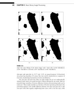
FIGURE 13.4
(a) Original binary image (192 ϫ 228 pixels) and a square marker within the largest component.
The next three images show iterations of the conditional dilation of the marker with a 3 ϫ 3-
pixel square structuring element; (b) 10 iterations; (c) 40 iterations; (d) reconstruction opening,
reached after 128 iterations.
Replacing the binary with gray-level images, the set dilation with function dilation,
and ∩with ∧yields the gray-level reconstruction opening of a gray-level image f from a
marker image m:
␳
Ϫ
B
(m|f ) ϭ lim
k→ϱ
g
k
, g
k
ϭ ␦
B
( g
kϪ1
) ∧f , g
0
ϭ m Յ f . (13.30)
This reconstructs the bright components of the reference image f that contains the
marker m. For example, as shown in Fig. 13.2, the results of any prior image smoothing,
like the radial opening of Fig. 13.2(b), can be treated as a marker which is subsequently

reconstructed under the original image as reference to recover exactly those bright image
components whose parts have remained after the first operation.
There is a large variety of reconstruction openings depending on the choice of the
marker. Two useful cases are (i) size-based markers chosen as the Minkowski erosion
m ϭ f rB of the reference image f by a disk of radius r and (ii) contrast-based markers
chosen as the difference m(x) ϭ f (x) Ϫ h of a constant h > 0 from the image. In the
first case, the reconstruction opening retains only objects whose horizontal size (i.e.,
diameter of inscribable disk) is not smaller than r. In the second case, only objects whose
contrast (i.e., height difference from neighbors) exceeds h will leave a remnant after the
reconstruction. In both cases, the marker is a function of the reference signal.
Reconstruction of the dark image components hit by some marker is accomplished
by the dual filter, the reconstr uction closing,
␳
ϩ
B
(m|f ) ϭ lim
k→ϱ
g
k
, g
k
ϭ ␧
B
( g
kϪ1
) ∨f , g
0
ϭ m Ն f . (13.31)
Examples of gray-level reconstruction filters are shown in Fig. 13.5.
Despite their many applications, reconstruction openings and closings ␺ have as a

disadvantage the property that they are not self-dual operators; hence, they t reat the
image and its background asymmetrically. A newer operator type that unifies both
of them and possesses self-duality is the leveling [14]. Levelings are nonlinear object-
oriented filters that simplify a reference image f through a simultaneous use of locally
13.3 Morphological Filters for Image Enhancement 305
(a) (b) (c)
0 0.2 0.4 0.6 0.8 0.9
Ϫ1
0
0.5
1
Reference, Marker & Rec.opening
Ϫ0.5
0
0.5
1
1 0 0.2 0.4 0.6 0.8 0.9 1
Ϫ1
Ϫ0.5
0
0.5
1
Reference, Marker & Rec.closing
0 0.2 0.4 0.6 0.8 0.9 1
Ϫ1
Ϫ0.5
0
0.5
1
Reference, Marker & Leveling

FIGURE 13.5
Reconstruction filters for 1D images. Each figure shows reference signals f (dash), markers (thin
solid), and reconstructions (thick solid). (a) Reconstruction opening from marker ϭ (f B) Ϫ const;
(b) Reconstruction closing from marker ϭ (f ⊕B) ϩ const; (c) Leveling (self-dual reconstruction) from
an arbitrary marker.
expanding and shrinking an initial seed image, called the marker m, and global con-
straining of the marker evolution by the reference image. Specifically, iterations of the
image operator ␭(m|f ) ϭ ( ␦
B
(m) ∧f ) ∨ ␧
B
(m),where ␦
B
(·) (respectively ␧
B
(·))isa
dilation (respectively erosion) by the unit-radius discrete disk B of the grid, yield in the
limit the leveling of f w.r.t. m:
⌳
B
(m|f ) ϭ lim
k→ϱ
g
k
, g
k
ϭ

␦
B

( g
kϪ1
) ∧f

∨ ␧
B
( g
kϪ1
), g
0
ϭ m. (13.32)
In contrast to the reconstruction opening (closing) where the marker m is smaller
(greater) than f , the marker for a general leveling may have an arbitrary ordering w.r.t.
the reference signal (see Fig. 13.5(c)). The leveling reduces to being a reconstruction
opening (closing) over regions where the marker is smaller ( greater) than the reference
image.
If the marker is self-dual, then the leveling is a self-dual filter and hence treats sym-
metrically the brig ht and dark objects in the image. Thus, the leveling may be called a
self-dual reconstruction filter. It simplifies both the original image and its backg round by
completely eliminating smaller objects inside which the marker cannot fit. The reference
image plays the role of a global constraint.
In general, levelings have many interesting multiscale properties [14]. For example,
they preserve the coupling and sense of variation in neighbor image values and do not
create any new regional maxima or minima. Also, they are increasing and idempotent
filters. They have proven to be very useful for image simplification toward segmentation
because they can suppress small-scale noise or small features and keep only large-scale
objects with exact preservation of their boundaries.
13.3.3 Contrast Enhancement
Imagine a gray-level image f that has resulted from blurring an original image g by
linearly convolving it with a Gaussian function of variance 2t . This Gaussian blurring

306 CHAPTER 13 Morphological Filtering
can be modeled by running the classic heat diffusion differential equation for the time
interval [0,t ]starting from the initial condition g at t ϭ 0. If we can reverse in time this
diffusion process, then we can deblur and sharpen the blurred image. By approximating
the spatio-temporal derivatives of the heat equation with differences, we can derive a
linear discrete filter that can enhance the contrast of the blurred image f by subtracting
from f a discretized version of its Laplacian ٌ
2
f ϭ Ѩ
2
f /Ѩx
2
ϩ Ѩ
2
f /Ѩy
2
. This is a simple
linear deblurring scheme, called unsharp constrast enhancement. A conceptually similar
procedure is the following nonlinear filtering scheme.
Consider a gray-level image f [x] and a small-size symmetric disk-like structuring
element B containing the origin. The following discrete nonlinear filter [15] can enhance
the local contrast of f by sharpening its edges:
␺( f )[x]ϭ
⎧
⎨
⎩
( f ⊕B)[x] if f [x]Ն (( f ⊕B)[x]ϩ ( f B)[x])/2
( f B)[x] if f [x]<((f ⊕B)[x]ϩ ( f B)[x])/2.
(13.33)
At each pixel x, the output value of this filter toggles between the value of the dilation of

f by B (i.e., the maximum of f inside the moving window B centered) at x and the value
of its erosion by B (i.e., the minimum of f within the same window) according to which
is closer to the input value f [x]. The toggle filter is usually applied not only once but
is iterated. The more iterations, the more contrast enhancement. Further, the iterations
converge to a limit (fixed point) [15] reached after a finite number of iterations. Examples
are shown in Figs. 13.6 and 13.7.
(a) Original and Gauss–blurred signal
Sam
p
le index
0 200 400 600 800 1000
21
20.5
0
0.5
1
(b)
Toggle filter iterations
Sam
p
le index
0 200 400 600 800 1000
21
20.5
0
0.5
1
FIGURE 13.6
(a) Original signal (dashed line) f [x]ϭ sign(cos(4␲x)), x ∈[0,1], and its blurring (solid line) via
convolution with a truncated sampled Gaussian function of ␴ ϭ 40; (b) Filtered versions (dashed

lines) of the blurred signal in (a) produced by iterating the 1D toggle filter (with B ϭ {Ϫ1,0,1})
until convergence to the limit signal (thick solid line) reached at 66 iterations; the displayed
filtered signals correspond to iteration indexes that are multiples of 20.
13.4 Morphological Operators for Template Matching 307
(a) (b) (c) (d)
FIGURE 13.7
(a) Original image f ; (b) Blurred image g obtained by an out-of-focus camera digitizing f ; (c) Out-
put of the 2D toggle filter acting on g (B was a small symmetric disk-like set); (d) Limit of iterations
of the toggle filter on g (reached at 150 iterations).
13.4 MORPHOLOGICAL OPERATORS FOR TEMPLATE MATCHING
13.4.1 Morphological Correlation
Consider two real-valued discrete image signals f [x] and g[x]. Assume that g is a signal
pattern to be found in f . To find which shifted version of g “best” matches f , a standard
approach has been to search for the shift lag y that minimizes the mean-squared error,
E
2
[y]ϭ

x∈W
( f [x ϩ y]Ϫ g [x])
2
, over some subset W of Z
2
. Under certain assump-
tions, this matching criterion is equivalent to maximizing the linear cross-correlation
L
fg
[y] 

x∈W

f [x ϩ y]g[x]between f and g .
Although less mathematically tractable than the mean squared error criterion, a statis-
tically more robust criterion is to minimize the mean absolute error,
E
1
[y]ϭ

x∈W
|f [x ϩ y]Ϫ g [x]|.
This mean absolute error criterion corresponds to a nonlinear signal correlation used
for signal matching; see [6] for a review. Specifically, since |a Ϫ b| ϭ a ϩ b Ϫ 2min(a,b),
under certain assumptions (e.g., if the error norm and the correlation is normalized by
dividing it with the average area under the signals f and g ),minimizing E
1
[y]is equivalent
to maximizing the morphological cross-correlation:
M
fg
[y] 

x∈W
min( f [x ϩ y],g[x]). (13.34)
It can be shown experimentally and theoretically that the detection of g in f is indicated
by a sharper matching peak in M
fg
[y]than in L
fg
[y]. In addition, the morphological (sum
of minima) correlation is faster than the linear (sum of products) correlation. These two
advantages of the morphological correlation coupled with the relative robustness of the

mean absolute error criterion make it promising for general signal matching.
308 CHAPTER 13 Morphological Filtering
13.4.2 Binary Object Detection and Rank Filtering
Let us approach the problem of binary image object detection in the presence of noise
from the viewpoint of statistical hypothesis testing and rank filtering. Assume that the
observed discrete binary image f [x] within a mask W has been generated under one of
the following two probabilistic hypotheses:
H
0
: f [x]ϭ e[x], x ∈ W ,
H
1
: f [x]ϭ |g[x Ϫ y]Ϫ e[x]|, x ∈W .
Hypothesis H
1
(H
0
) stands for “object present” (“object not present”) at pixel location y.
The object g[x] is a deterministic binary template. The noise e[x] is a stationary binary
random field which is a 2D sequence of i.i.d. random variables taking value 1 with
probability p and 0 with probability 1 Ϫ p, where 0 < p < 0.5. The mask W ϭ G
ϩy
is a
finite set of pixels equal to the reg i on G of support of g shifted to location y at which the
decision is taken. (For notational simplicity, G is assumed to be symmetric, i.e., G ϭ G
s
.)
The absolute-difference superposition between g and e under H
1
forces f to always have

values 0 or 1. Intuitively, such a signal/noise superposition means that the noise e toggles
the value of g from 1 to 0 and from 0 to 1 with probability p at each pixel. This noise
model can be viewed either as the common binary symmetric channel noise in signal
transmission or as a binary version of the salt-and-pepper noise. To decide whether the
object g occurs at y, we use a Bayes decision rule that minimizes the total probability of
error and hence leads to the likelihood ratio test :
Pr(f /H
1
)
Pr(f /H
0
)
H
1
>
<
H
0
Pr(H
0
)
Pr(H
1
)
, (13.35)
where Pr( f /H
i
) are the likelihoods of H
i
with respect to the observed image f , and

Pr(H
i
) are the a pr iori probabilities. This is equivalent to
M
fg
[y]ϭ

x∈W
min( f [x],g[x Ϫ y])
H
1
>
<
H
0
␪ ϭ
1
2

log [Pr (H
0
)/Pr(H
1
)]
log [(1 Ϫ p)/p]
ϩ card(G)

. (13.36)
Thus, the selected statistical criterion and noise model lead to computing the morpho-
logical (or equivalently linear) binary correlation between a noisy image and a known

image object and comparing it to a threshold for deciding whether the object is present.
Thus, optimum detection in a binary image f of the presence of a binary object g
requires comparing the binary correlation between f and g to a threshold ␪. This is
equivalent
4
to performing a r-th rank filtering on f byasetG equal to the support of
4
An alternative implementation and view of binary rank filtering is via thresholded convolutions, where a
binary image is linearly convolved with the indicator function of a set G with n ϭ card( G) pixels, and then
the result is thresholded at an integer level r between 1 and n; this yields the output of the r-th rank filter
by G acting on the input image.
13.5 Morphological Operators for Feature Detection 309
g , where 1 Յ r Յ card( G) and r is related to ␪. Thus, the rank r reflects the area portion
of (or a probabilistic confidence score for) the shifted template existing around pixel y.
For example, if Pr(H
0
) ϭ Pr(H
1
), then r ϭ ␪ ϭ card(G)/2, and hence the binary median
filter by G becomes the optimum detector.
13.4.3 Hit-Miss Filter
The set erosion (13.3) can also be viewed as Boolean template matching since it gives
the center points at which the shifted structuring element fits inside the image object.
If we now consider a set A probing the image object X and another set B probing the
background X
c
, the set of points at which the shifted pair (A,B) fits inside the image X
is the hit-miss transformat ion of X by (A, B):
X ⊗(A,B)  {x : A
ϩx

⊆ X, B
ϩx
⊆ X
c
}. (13.37)
In the discrete case, this can be represented by a Boolean product function whose uncom-
plemented (complemented) variables correspond to points of A (B). It has been used
extensively for binary feature detection [2]. It can actually model all binary template
matching schemes in binary pattern recognition that use a pair of a positive and a
negative template [3].
In the presence of noise, the hit-miss filter can be made more robust by replacing the
erosions in its definitions with rank filters that do not require an exact fitting of the whole
template pair (A,B) inside the image but only a part of it.
13.5 MORPHOLOGICAL OPERATORS FOR FEATURE DETECTION
13.5.1 Edge Detection
By image edges we define abrupt intensity changes of an image. Intensity changes usually
correspond to physical changes in some property of the imaged 3D objects’ surfaces (e.g.,
changes in reflectance, texture, depth or orientation discontinuities, object boundaries)
or changes in their illumination. Thus, edge detection is very important for subsequent
higher level vision tasks and can lead to some inference about physical properties of the
3D world. Edge types may be classified into three types by approximating their shape
with three idealized patterns: lines, steps, and roofs, which correspond, respectively, to
the existence of a Dirac impulse in the derivative of order 0, 1, and 2. Next we focus
mainly on step edges. The problem of edge detection can be separated into three main
subproblems:
1. Smoothing: image intensities are smoothed via filtering or approximated by
smooth analytic functions. The main motivations are to suppress noise and
decompose edges at multiple scales.
2. Differentiation: amplifies the edges and creates more easily detectable simple
geometric patterns.

310 CHAPTER 13 Morphological Filtering
3. Decision: edges are detected as peaks in the magnitude of the first-order derivatives
or zero-crossings in the second-order derivatives, both compared with some
threshold.
Smoothing and differentiation can be either linear or nonlinear. Further, the dif-
ferentiation can be either directional or isotropic. Next, after a brief synopsis of the
main linear approaches for edge detection, we describe some fully nonlinear ones using
morphological gradient-type residuals.
13.5.1.1 Linear Edge Operators
In linear edge detection, both smoothing and differentiation are done via linear convolu-
tions. These two stages of smoothing and differentiation can be done in a single stage of
convolution with the derivative of the smoothing kernel. Three well-known approaches
for edge detection using linear operators in the main stages are the following:
■ Convolution with edge templates: Historically, the first approach for edge detec-
tion, which lasted for about three decades (1950s–1970s), was to use discrete
approximations to the image linear partial derivatives, f
x
ϭ Ѩf /Ѩx and f
y
ϭ Ѩf /Ѩy,
by convolving the digital image f with very small e dge-enhancing kernels. Exam-
ples include the Prewitt, Sobel and Kirsch edge convolution masks reviewed in
[3, 16]. Then these approximations to f
x
,f
y
were combined nonlinearly to give a
gradient magnitude ||ٌf || using the 
1
, 

2
,or
ϱ
norm. Finally, peaks in this edge
gradient magnitude were detected, via thresholding, for a binary edge decision.
Alternatively, edges were identified as zero-crossings in second-order derivatives
which were approximated by small convolution masks acting as digital Laplacians.
All these above approaches do not perform well because the resulting convolution
masks act as poor digital highpass filters that amplify high-frequency noise and do
not provide a scale localization/selection.
■ Zero-crossings of Laplacian-of-Gaussian convolution: Marr and Hildreth [17]
developed a theory of edge detection based on evidence from biological vision sys-
tems and ideas from signal theory. For image smoothing, they chose linear convolu-
tions with isotropic Gaussian functions G
␴
(x,y) ϭ exp[Ϫ(x
2
ϩ y
2
)/2␴
2
]/(2␲␴
2
)
to optimally localize edges both in the space and frequency domains. For differ-
entiation, the y chose the Laplacian operator ٌ
2
since it is the only isotropic linear
second-order differential operator. The combination of Gaussian smoothing and
Laplacian can be done using a sing le convolution with a Laplacian-of-Gaussian

(LoG) kernel, which is an approximate bandpass filter that isolates from the origi-
nal image a scale band on which edges are detected. The scale is determined by ␴.
Thus, the image edges are defined as the zero-crossings of the image convolution
with a LoG kernel. In practice, one does not accept all zero-crossings in the LoG
output as edge points but tests whether the slope of the LoG output exceeds a
certain threshold.
■ Zero-crossings of directional derivatives of smoothed image: For detecting edges
in 1D signals corrupted by noise, Canny [18] developed an optimal approach where
13.5 Morphological Operators for Feature Detection 311
edges were detected as maxima in the output of a linear convolution of the signal
with a finite-extent impulse response h. By maximizing the following figures of
merit, (i) good detection in terms of robustness to noise, (ii) good edge localization,
and (iii) uniqueness of the result in the vicinity of the edge, he found an optimum
filter with an impulse response h(x) which can be closely approximated by the
derivative of a Gaussian. For 2D images, the Canny edge detector consists of three
steps: (1) smooth the image f (x,y) with an isotropic 2D Gaussian G
␴
, (2) find
the zero-crossings of the second-order directional derivative Ѩ
2
f /Ѩ␩
2
of the image
in the direction of the gr adient ␩ ϭٌf /||ٌf ||, (3) keep only those zero-crossings
and declare them as edge pixels if they belong to connected arcs whose points
possess edge strengths that pass a double-threshold hysteresis criterion. Closely
related to Canny’s edge detector was Haralick’s previous work (reviewed in [16])
to regularize the 2D discrete image function by fitting to it bicubic interpolating
polynomials, compute the image derivatives from the interpolating polynomial,
and find the edges as the zero-crossings of the second directional derivative in the

gradient direction. The Haralick-Canny edge detector yields different and usually
better edges than the Marr-Hildreth detector.
13.5.1.2 Morphological Edge Detection
The boundary of a set X ⊆ R
m
, m ϭ 1,2, ,isgivenby
ѨX  X \
◦
X
ϭ
X ∩(
◦
X
)
c
, (13.38)
where X and
◦
X
denote the closure and interior of X.Now,if||x|| is the Euclidean norm
of x ∈R
m
, B is the unit ball, and rB ϭ {x ∈ R
m
: ||x||Յ r} is the ball of radius r, then it
can be shown that
ѨX ϭ

r>0
(X ⊕rB) \(X rB). (13.39)

Hence, the set difference between erosion and dilation can provide the “edge,” i.e., the
boundar y of a set X.
These ideas can also be extended to signals. Specifically, let us define morphological
sup-derivative M( f ) of a function f : R
m
→ R at a point x as
M( f )(x)  lim
r↓0
( f ⊕rB)(x) Ϫ f (x)
r
ϭ lim
r↓0

||y||Յr
f (x ϩ y) Ϫ f (x)
r
. (13.40)
By applying M to Ϫf and using the duality between dilation and erosion, we obtain
the inf-derivative of f . Suppose now that f is differentiable at x ϭ (x
1
, ,x
m
) and let its
gradient be ٌf ϭ

Ѩf
Ѩx
1
, ,
Ѩf

Ѩx
m

. Then it can be shown that
M( f )(x) ϭ ||ٌf (x)||. (13.41)
Next, if we take the difference between sup-derivative and inf-derivative when the scale
goes to zero, we arrive at an isotropic second-order morphological derivative:
M
2
( f )(x)  lim
r↓0
[( f ⊕rB)(x) Ϫ f (x)]Ϫ [f (x) Ϫ (f rB)(x)]
r
2
. (13.42)
312 CHAPTER 13 Morphological Filtering
The peak in the first-order morphological derivative or the zero-crossing in the
second-order morphological derivative can detect the location of an edge, in a similar
way as the traditional linear derivatives can detect an edge.
By approximating the morphological derivatives with differences, various simple and
effective schemes can be developed for extracting edges in digital images. For example, for
a binary discrete image represented as a set X in Z
2
, the set difference (X ⊕B) \(X B)
gives the boundary of X.HereB equals the 5-pixel rhombus or 9-pixel square depending
on whether we desire 8- or 4-connected image boundaries. An asymmetric treatment
between the image foreground and background results if the dilation difference (X ⊕
B) \X or the erosion difference X \(X B) is applied, because they yield a boundary
belonging only to X
c

or to X , respectively.
Similar ideas apply to gray-level images. Both the dilation residual and the erosion
residual,
edge
⊕
( f )  (f ⊕B) Ϫ f , edge

( f )  f Ϫ (f B), (13.43)
enhance the edges of a gray-level image f . Adding these two operators yields the discrete
morphological gradient,
edge( f )  (f ⊕B) Ϫ (f B) ϭ edge
⊕
( f ) ϩ edge

( f ), (13.44)
that treats more symmetr ically the image and its background (see Fig. 13.8).
Threshold analysis can be used to understand the action of the above edge operators.
Let the nonnegative discrete-valued image signal f (x) have L ϩ 1 possible integer inten-
sity values: i ϭ 0,1, , L. By thresholding f at all levels, we obtain the threshold binary
images f
i
from which we can resynthesize f via threshold-sum sig nal superposition:
f (x) ϭ
L

iϭ1
f
i
(x), f
i

(x) ϭ

1, if f (x) Ն i
0, if f (x)<i·
(13.45)
Since the flat dilation and erosion by a finite B commute with thresholding and f is
nonnegative, they obey threshold-sum superposition. Therefore, the dilation-erosion
difference oper ator also obeys threshold-sum superposition:
edge( f ) ϭ
L

iϭ1
edge( f
i
) ϭ
m

iϭ1
f
i
⊕B Ϫ f
i
B. (13.46)
This implies that the output of the edge oper ator acting on the gray-level image f is
equal to the sum of the binary signals that are the boundaries of the binary images f (see
Fig. 13.8). At each pixel x, the larger the gradient of f , the larger the number of threshold
levels i such that edge(f
i
)(x) ϭ 1, and hence the larger the value of the gray-level signal
edge( f )(x). Finally, a binarized edge image can be obtained by thresholding edge( f ) or

detecting its peaks.
The morphological digital edge operators have been extensively applied to image
processing by many researchers. By combining the erosion and dilation differences, var-
ious other effective edge operators have also been developed. Examples include 1) the
13.5 Morphological Operators for Feature Detection 313
(a) (b)
(c) (d)
FIGURE 13.8
(a) Original image f with range in [0, 255]; (b) f ⊕B Ϫ f B, where B is a 3 ϫ 3-pixel square;
(c) Level set X ϭ X
i
( f ) of f at level i ϭ 100; (d) X ⊕B \X B; (In (c) and (d), black areas
represent the sets, while white areas are the complements.)
asymme tric morphological edge-strength operators by Lee et al. [19],
min[edge

( f ), edge
⊕
( f )], max[edge

( f ), edge
⊕
( f )], (13.47)
and 2) the edge operator edge
⊕
( f ) Ϫ edge

( f ) by Vliet et al. [20], which behaves as a
discrete “nonlinear Laplacian,”
NL( f ) ϭ (f ⊕B) ϩ (f B) Ϫ 2f , (13.48)

314 CHAPTER 13 Morphological Filtering
and at its zero-crossings can yield edge locations. Actually, for a 1D twice differentiable
function f (x), it can be shown that if df (x)/dx ϭ 0 then M
2
( f )(x) ϭ d
2
f (x)/dx
2
.
For robustness in the presence of noise, these morphological edge operators should
be applied after the input image has been smoothed fi rst via either linear or nonlinear
filtering. For example, in [19], a small local averaging is used on f before applying the
morphological edge-strength operator, resulting in the so-called min-blur edge detection
operator,
min[f
av
Ϫ f
av
B,f
av
⊕B Ϫ f
av
], (13.49)
with f
av
being the local average of f , whereas in [21] an opening and closing is used
instead of linear preaveraging:
min[f ◦B Ϫ f B,f ⊕B Ϫ f •B]. (13.50)
Combinations of such smoothings and morphological first or second derivatives have
performed better in detecting edges of noisy images. See Fig. 13.9 for an experimental

comparison of the LoG and the morphological second derivative in detecting edges.
13.5.2 Peak / Valley Blob Detection
Residuals between opening s or closings and the original image offer an intuitively simple
and mathematically formal way for peak or valley detection. The general principle for
peak detection is to subtract from a signal an opening of it. If the latter is a standard
Minkowski opening by a flat compact convex set B, then this yields the peaks of the
signal whose base cannot contain B. The morphological peak/valley detectors are simple,
efficient, and have some advantages over curvature-based approaches. Their applicability
in situations where the peaks or valleys are not clearly separated from their surroundings
is further strengthened by generalizing them in the following way. The conventional
Minkowski opening in peak detection is replaced by a general lattice opening, usually
of the reconstruction type. This generalization allows a more effective estimation of the
image background surroundings around the peak and hence a better detection of the
peak. Next we discuss peak detectors based on both the standard Minkowski openings
as well as on generalized lattice openings like contrast-based reconstructions which can
control the peak height.
13.5.2.1 Top-Hat Transformation
Subtracting from a signal f its Minkowski opening by a compact convex set B yields an
output consisting of the signal peaks whose supports cannot contain B. This is Meyer’s
top-hat transformation [22], implemented by the opening residual,
peak( f )  f Ϫ (f ◦B), (13.51)
13.5 Morphological Operators for Feature Detection 315
Original image N2 = Gauss noise 20 dB N1 = Gauss noise 6 dB
Ideal edges
LoG edges (N2)
LoG edges (N1)
Ideal edges
MLG edges (N2) MLG edges (N1)
FIGURE 13.9
Top: Test image and two noisy versions with additive Gaussian noise at SNR 20 dB and 6 dB.

Middle: Ideal edges and edges from zero-crossings of Laplacian-of-Gaussian of the two noisy
images. Bottom:Ideal edges and edges fromzero-crossings of 2D morphological secondderivative
(nonlinear Laplacian) of the twonoisy images aftersome Gaussian presmoothing.In both methods,
the edge pixels were the subset of the zero-crossings where the edge strength exceeded some
threshold. By using as figure-of-merit the average of the probability of detecting an edge given
that it is true and the probability of a true edge given than it is detected, the morphological method
scored better by yielding detection probabilities of 0.84 and 0.63 at the noise levels of 20 and 6
dB, respectively, whereas the corresponding probabilities of the LoG method were 0.81 and 0.52.
and henceforth called the peak operator. The output peak(f ) is always a nonnegative
signal, which guarantees that it contains only peaks. Obviously the set B is a very impor-
tant parameter of the peak operator, because the shape and size of the peak’s support
obtained by (13.51) are controlled by the shape and size of B. Similarly, to extract the
valleys of a signal f , we can apply the closing residual,
valley( f )  ( f •B) Ϫ f , (13.52)
henceforth called the valley operator.
316 CHAPTER 13 Morphological Filtering
If f is an intensity image, then the opening (or closing) residual is a very useful
operator for detecting blobs, defined as regions with significantly brighter (or darker)
intensities relative to the surroundings. Examples are shown in Fig. 13.10.
If the sig nal f (x) assumes only the values 0,1, ,L and we consider its threshold
binary signals f
i
(x) definedin (13.45), then since theopening by f ◦B obeys the threshold-
sum superposition,
peak( f ) ϭ
L

iϭ1
peak( f
i

). (13.53)
Thus the peak operator obeys threshold-sum superposition. Hence, its output when
operating on a gray-level signal f is the sum of its binary outputs when it operates on all
the threshold binary versions of f . Note that, for each binary signal f
i
, the binar y output
peak (f
i
) contains only those nonzero parts of f
i
inside which no translation of B fits.
The morphological peak and valley operators, in addition to being simple and
efficient, avoid several shortcomings of the curvature-based approaches to peak/valley
extraction that can be found in earlier computer vision literature. A differential geometry
interpretation of the morphological feature detectors was given by Noble [23], who also
developed and analyzed simple operators based on residuals from openings and closings
to detect corners and junctions.
13.5.2.2 Dome/Basin Extraction with Reconstruction Opening
Extracting the peaks of a signal via the simple top-hat operator (13.51) does not constrain
the height of the resulting peaks. Specifically, the threshold-sum superposition of the
opening difference in (13.53) implies that the peak heig ht at each point is the sum of all
binary peak signals at this point. In several applications, however, it is desirable to extract
from a signal f peaks that have a maximum height h > 0. Such peaks are called domes
and are defined as follows. Subtracting a contrast height constant h from f (x) yields the
smaller signal g(x) ϭ f (x) Ϫ h < f (x). Enlarging the maximum peak value of g below
(a) (b) (c) (d)
FIGURE 13.10
Facial image feature extraction. (a) Original image f ; (b) Morphological gradient f ⊕B Ϫ f B;
(c) Peaks: f Ϫ (f
◦3B); (d) Valleys: (f •3B) Ϫ f (B is 21-pixel octagon).

13.6 Design Approaches for Morphological Filters 317
a peak of f by locally dilating g with a symmetric compact and convex set of an e ver-
increasing diameter and always restricting these dilations to never produce a signal larger
than f under this specific peak produces in the limit a signal which consists of valleys
interleaved with flat plateaus. This signal is the reconstruction opening of g under f ,
denoted as ␳
Ϫ
( g |f ); namely, f is the reference signal and g is the marker. Subtracting the
reconstruction opening from f yields the domes of f , defined in [24] as the generalized
top-hat:
dome( f )  f Ϫ ␳
Ϫ
( f Ϫ h|f ). (13.54)
For discrete-domain signals f , the above reconstruction opening can be implemented
by iterating the conditional dilation as in (13.30). This is a simple but computationally
expensive algorithm. More efficient algorithms can be found in [24, 25]. The dome
operator extracts peaks whose height cannot exceed h but their supports can be arbitrarily
wide. In contrast, the peak operator (using the opening residual) extracts peaks whose
supports cannot exceed a set B but their heights are unconstrained.
Similarly, an operator can be defined that extracts signal valleys whose depth cannot
exceed a desired maximum h. Such valleys are called basins and are defined as the domes
of the negated signal. By using the duality between morphological operations, it can be
shown that basins of height h can be extracted by subtracting the original image f (x)
from its reconstruction closing obtained using as marker the signal f (x) ϩ h:
basin( f )  dome(Ϫf ) ϭ ␳
ϩ
( f ϩ h|f ) Ϫ f . (13.55)
Domes and basins have found numerous applications as region-based image features and
as markers in image segmentation tasks. Several successful paradigms are discussed in
[24–26].

The following example, adapted from [24], illustrates that domes perform better
than the classic top-hat in extracting small isolated peaks that indicate pathology points
in biomedical images, e.g., detect microaneurisms in eye angiograms without confusing
them with the large vessels in the eye image (see Fig. 13.11).
13.6 DESIGN APPROACHES FOR MORPHOLOGICAL FILTERS
Morphological and rank/stack filters are useful for image enhancement and are closely
related since they can all be represented as maxima of morphological erosions [5]. Despite
the wide application of these nonlinear filters,very few ideas exist for their optimal design.
The current four main approaches are as follows: (a) designing morphological filters as
a finite union of erosions [27] based on the morphological basis representation the-
ory (outlined in Section 13.2.3); (b) designing stack filters via threshold decomposition
and linear programming [9]; (c) designing morphological networks using either voting
logic and rank tracing learning or simulated annealing [28]; (d) designing morphologi-
cal/rank filters via a g radient-based adaptive optimization [29]. Approach (a) is limited
to binary increasing filters. Approach (b) is limited to increasing filters processing non-
negative quantized signals. Approach (c) needs a long time to train and convergence is
318 CHAPTER 13 Morphological Filtering
Original image = F
Reconstruction opening (F – h| F)
Reconstr. opening (rad.open|F)
Top hat: Peaks
New top hat: Domes
Final top hat
Threshold peaks
Threshold domes
Threshold final top hat
FIGURE 13.11
Top row: Original image F of eye angiogram with microaneurisms, its top hat F Ϫ F◦B, where
B is a disk of radius 5, and level set of top hat at height h/2. Middle row: Reconstruction
opening ␳

Ϫ
(F Ϫ h|F), domes F Ϫ ␳
Ϫ
(F Ϫ h|F), level set of domes at height h/2. Bottom row:
New reconstruction opening of F using the radial opening of Fig. 13.2(b) as marker, new domes,
and level set detecting microaneurisms.
complex. In contrast, approach (d) is more general since it applies to both increasing and
non-increasing filters and to both binary and real-valued signals. The major difficulty
involved is that rank functions are not differentiable, which imposes a deadlock on how
to adapt the coefficients of morphological/rank filters using a gradient-based algorithm.
References 319
The methodology described in this section is an extension and improvement to the
design methodolog y (d), leading to a new approach that is simpler, more intuitive, and
numerically more robust.
For various signal processing applications, it is sometimes useful to mix in the same
system both nonlinear and linear filtering strategies. Thus, hybrid systems, composed
of linear and nonlinear (rank-type) sub-systems, have frequently been proposed in the
research literature. A typical example is the class of L-filters that are linear combinations
of rank filters. Several adaptive algorithms have also been developed for their design,
which illustrated the potential of adaptive hybrid filters for image processing applications,
especially in the presence of non-Gaussian noise.
Another example of hybrid systems are the morphological/rank/linear (MRL) filters
[30], which contain as special cases morphological, rank, and linear filters. These MRL
filters consist of a linear combination between a morphological/rank filter and a linear
finite impulse response filter. Their nonlinear component is based on a rank function,
from which the basic morphological operators of erosion and dilation can be obtained
as special cases. An efficient method for their adaptive optimal design can be found
in [30].
13.7 CONCLUSIONS
In this chapter, we have briefly presented the application of both the standard and some

advanced morphological filters to several problems of image enhancement and feature
detection. There are several motivations for using morphological filters for such prob-
lems. First, it is of paramount importance to preserve, uncover, or detect the geometric
structure of image objects. Thus,morphological filters which are more suitablethan linear
filters for shape analysis, play a major role for geometry-based enhancement and detec-
tion. Further, they offer efficient solutions to other nonlinear tasks such as non-Gaussian
noise suppression. Although this denoising task can also be accomplished (with similar
improvements over linear filters) by the closely related class of median-type and stack
filters, the morphological operators provide the additional feature of geometric intuition.
Finally, the elementary morphological operators are the building blocks for large classes
of nonlinear image processing systems, which include rank and stack filters.
Three important broad research directions in morphological filtering are (1) their
optimal design for various advanced image analysis and vision tasks, (2) their scale-space
formulation using geometric partial differential equations (PDEs), and (3) their isotropic
implementation using numerical algorithms that solve these PDEs. A survey of the last
two topics can be found in [31].
REFERENCES
[1] G. Matheron. Random Sets and Integral Geometry. John Wiley and Sons, NY, 1975.
[2] J. Serra. Image Analysis and Mathematical Morphology. Academic Press, Burlington, MA, 1982.
320 CHAPTER 13 Morphological Filtering
[3] A. Rosenfeld and A. C. Kak. Digital Picture Processing, Vols. 1 & 2. Academic Press, Boston, MA,
1982.
[4] K. Preston, Jr. and M. J. B. Duff. Modern Cellular Automata. Plenum Press, NY, 1984.
[5] P. Maragos and R. W. Schafer. Morphological filters. Part I: their set-theoretic analysis and relations
to linear shift-invariant filters. Part II: their relations to median, order-statistic, and stack filters.
IEEE Trans. Acoust., 35:1153–1184, 1987; ibid, 37:597, 1989.
[6] P. Maragos and R. W. Schafer. Morphological systems for multidimensional signal processing. Proc.
IEEE, 78:690–710, 1990.
[7] J. Serra, editor. Image Analysis and Mathematical Morphology,Vol. 2: Theoretical Advances. Academic
Press, Burlington, MA, 1988.

[8] H. J. A. M. Heijmans. Morphological Image Operators. Academic Press, Boston, MA, 1994.
[9] E. J. Coyle and J. H. Lin. Stack filters and the mean absolute error criterion. IEEE Trans. Acoust.,
36:1244–1254, 1988.
[10] N. D. Sidiropoulos, J. S. Baras, and C. A. Berenstein. Optimal filtering of digital binary images
corrupted by union/intersection noise. IEEE Trans. Image Process., 3:382–403, 1994.
[11] D. Schonfeld and J. Goutsias. Optimal morphological pattern restoration from noisy binary images.
IEEE Trans. Pattern Anal. Mach. Intell., 13:14–29, 1991.
[12] J. Serra and P. Salembier. Connected operators and pyramids. In Proc. SPIE Vol. 2030, Image Algebra
and Mathematical Morphology, 65–76, 1993.
[13] P. Salembier and J. Serra. Flat zones filtering, connected operators, and filters by reconstruction.
IEEE Trans. Image Process., 4:1153–1160, 1995.
[14] F. Meyer and P. Maragos. Nonlinear scale-space representation with morphological levelings.
J. Visual Commun. Image Representation, 11:245–265, 2000.
[15] H. P. Kramer and J. B. Bruckner. Iterations of a nonlinear transformation for enhancement of
digital images. Pattern Recognit., 7:53–58, 1975.
[16] R. M. Haralick and L. G. Shapiro. Computer and Robot Vision, Vol. I. Addison-Wesley, Boston, MA,
1992.
[17] D. Marr and E. Hildreth. Theory of edge detection. Proc. R. Soc. Lond., B, Biol. Sci., 207:187–217,
1980.
[18] J. Canny. A computational approach to edge detection. IEEE Trans. Pattern Anal. Mach. Intell.,
PAMI-8:679–698, 1986.
[19] J. S. J. Lee, R. M. Haralick, and L. G. Shapiro. Morphologic edge detection. IEEE Trans. Rob. Autom.,
RA-3:142–156, 1987.
[20] L. J. van Vliet, I. T. Young, and G. L. Beckers. A nonlinear Laplace operator as edge detector in noisy
images. Comput. Vis., Graphics, and Image Process., 45:167–195, 1989.
[21] R. J. Feehs and G. R. Arce. Multidimensional morphological edge detection. In Proc. SPIE Vol. 845:
Visual Communications and Image Processing II, 285–292, 1987.
[22] F. Meyer. Contrast feature extraction. In Proc. 1977 European Symp. on Quantitative Analysis of
Microstructures in Materials Science, Biology and Medicine, France. Published in: Special Issues of
Practical Metallography, J. L. Chermant, editor, Riederer-Verlag, Stuttgart, 374–380, 1978.

[23] J. A. Noble. Morphological feature detection. In Proc. Int. Conf. Comput. Vis., Tarpon-Springs, FL,
1988.
References 321
[24] L. Vincent. Morphological g rayscale reconstruction in image analysis: applications and efficient
algorithms. IEEE Trans. Image Process., 2:176–201, 1993.
[25] P. Salembier. Region-based filtering of images and video sequences: a morphological view-point.
In S. K. Mitra and G. L. Sicuranza, editors, Nonlinear Image Processing, Academic Press,Burlington,
MA, 2001.
[26] A. Banerji and J. Goutsias. A morphological approach to automatic mine detection problems. IEEE
Trans. Aerosp. Electron Syst., 34:1085–1096, 1998.
[27] R. P. Loce and E. R. Doughert y. Facilitation of optimal binary morphological filter design via
structuring element libraries and design constraints. Opt. Eng., 31:1008–1025, 1992.
[28] S. S. Wilson. Training structuring elements in morphological networks. In E. R. Dougherty, editor,
Mathematical Morphology in Image Processing, Marcel Dekker, NY, 1993.
[29] P. Salembier. Adaptive rank order based filters. Signal Processing, 27:1–25, 1992.
[30] L. F. C. Pessoa and P. Maragos. MRL-filters: a general class of nonlinear systems and their optimal
design for image processing. IEEE Trans. Image Process., 7:966–978, 1998.
[31] P. Maragos. Partial differential equations for morphological scale-spaces and Eikonal applications.
In A. C. Bovik, editor, The Image and Video Processing Handbook, 2nd ed., 587–612. Elsevier
Academic Press, Burlington, MA, 2005.
CHAPTER
14
Basic Methods for Image
Restoration and
Identification
Reginald L. Lagendijk and Jan Biemond
Delft University of Technology, The Netherlands
14.1 INTRODUCTION
Images are produced to record or display useful information. Due to imperfections in
the imaging and capturing process, however, the recorded image invariably represents

a degraded version of the original scene. The undoing of these imperfections is cru-
cial to many of the subsequent image processing tasks. There exists a wide range of
different degradations that need to be taken into account, covering for instance noise,
geometrical degradations (pin cushion distortion), illumination and color imperfections
(under/overexposure, saturation), and blur. This chapter concentrates on basic methods
for removing blur from recorded sampled (spatially discrete) images. There are many
excellent overview articles, journal papers, and textbooks on the subject of image restora-
tion and identification. Readers interested in more details than given in this chapter are
referred to [1–5].
Blurring is a form of bandwidth reduction of an ideal image owing to the imperfect
image formation process. It can be caused by relative motion between the camera and the
original scene, or by an optical system that is out of focus. When aerial photographs are
produced for remote sensing purposes, blurs are introduced by atmospheric turbulence,
aberrations in the optical system, andrelative motionbetween the camera and the ground.
Such blurring is not confined to optical images; for example, electron micrographs are
corrupted by spherical aberrations of the electron lenses, and CT scans suffer from X-ray
scatter.
In addition to these blurring effects, noise always corrupts any recorded image. Noise
may be introduced by the medium through which the image is created (random absorp-
tion or scatter effects), by the recording medium (sensor noise), by measurement errors
due to the limited accuracy of the recording system, and by quantization of the data for
digital storage.
323
324 CHAPTER 14 Basic Methods for Image Restoration and Identification
The field of image restoration (sometimes referred to as image deblurring or image
deconvolution) is concerned with the reconstruction or estimation of the uncorrupted
image from a blurred and noisy one. Essentially, it tries to perform an operation on
the image that is the inverse of the imperfections in the image formation system. In
the use of image restoration methods, the characteristics of the deg rading system and the
noise are assumed to be known a priori. In practical situations, however, one may not be

able to obtain this information directly from the image formation process. The goal of
blur identification is to estimate the attributes of the imperfect imaging system from the
observed degraded image itself prior to the restoration process. Thecombination of image
restoration and blur identification is often referred to as blind image deconvolution [4].
Image restoration algorithms distinguish themselves from image enhancement meth-
ods in that they are based on m odels for the degrading process and for the ideal image.
For those cases where a fairly accurate blur model is available, powerful restoration
algorithms can be arrived at. Unfortunately, in numerous practical cases of interest, the
modeling of the blur is unfeasible, rendering restoration impossible. The limited validity
of blur models is often a factor of disappointment, but one should realize that if none
of the blur models described in this chapter are applicable, the corrupted image may
well be beyond restoration. Therefore, no matter how powerful blur identification and
restoration algorithms are, the objective when capturing an image undeniably is to avoid
the need for restoring the image.
The image restoration methods that are described in this chapter fall under the class
of linear spatially invariant restoration filters. We assume that the blurring function acts
as a convolution kernel or point-spread function d(n
1
,n
2
) that does not vary spatially.
It is also assumed that the statistical propert ies (mean and correlation function) of the
image and noise do not change spatially. Under these conditions the restoration process
can be carried out by means of a linear filter of which the point-spread function (PSF) is
spatially invariant, i.e., is constant throughout the image. These modeling assumptions
can be mathematically formulated as follows. If we denote by f (n
1
,n
2
) the desired ideal

spatially discrete image that does not contain any blur or noise, then the recorded image
g (n
1
,n
2
) is modeled as (see also Fig. 14.1(a)) [6]:
g (n
1
,n
2
) ϭ d(n
1
,n
2
) ∗f (n
1
,n
2
) ϩ w(n
1
,n
2
)
ϭ
N Ϫ1

k
1
ϭ0
MϪ1


k
2
ϭ0
d(k
1
,k
2
)f (n
1
Ϫ k
1
,n
2
Ϫ k
2
) ϩ w(n
1
,n
2
). (14.1)
Here w(n
1
,n
2
) is the noise that corrupts the blurred image. Clearly the objective of
image restoration is to make an estimate f (n
1
,n
2

) of the ideal image, given only the
degraded image g (n
1
,n
2
), the blurring function d(n
1
,n
2
), and some information about
the statistical properties of the ideal image and the noise.
An alternative way of describing (14.1) is through its spectral equivalence. By applying
discrete Fourier transforms to (14.1), we obtain the following representation (see also
Fig. 14.1(b)):
G(u,v) ϭ D(u , v)F(u, v) ϩ W (u,v), (14.2)
14.1 Introduction 325
G (u, v)
W (u, v)
F (u, v)
f (n
1
, n
2
)
g (n
1
, n
2
)
1

w (n
1
, n
2
)
1
Convolve with
d (n
1
, n
2
)
Multiply with
D (u, v)
(b)
(a)
FIGURE 14.1
(a) Image formation model in the spatial domain; (b) Image formation model in the Fourier
domain.
where (u,v) are the spatial frequency coordinates and capitals represent Fourier
transforms. Either (14.1) or (14.2) can be used for developing restoration algorithms.
In practice the spectral representation is more often used since it leads to efficient
implementations of restoration filters in the (discrete) Fourier domain.
In (14.1) and (14.2), the noise w(n
1
,n
2
) is modeled as an additive term. Typically
the noise is considered to have a zero-mean and to be white, i.e., spatially uncorrelated.
In statistical terms this can be expressed as follows [7]:

E
[
w(n
1
,n
2
)
]
≈
1
NM
N Ϫ1

k
1
ϭ0
MϪ1

k
2
ϭ0
w(k
1
,k
2
) ϭ 0 (14.3a)
R
w
(k
1

,k
2
) ϭ E
[
w(n
1
,n
2
)w(n
1
Ϫ k
1
,n
2
Ϫ k
2
)
]
≈
1
NM
N Ϫ1

n
1
ϭ0
MϪ1

n
2

ϭ0
w(n
1
,n
2
)w(n
1
Ϫ k
1
,n
2
Ϫ k
2
) ϭ

␴
2
w
if k
1
ϭ k
2
ϭ 0
0 elsewhere
. (14.3b)
Here ␴
2
w
is the variance or power of the noise and E[] refers to the expected value
operator. The approximate equality indicates that on the average Eq. (14.3) should hold,

but that for a given image Eq. (14.3) holds only approximately as a result of replacing the
expectation by a pixelwise summation over the image. Sometimes the noise is assumed
to have a Gaussian probability density function, but this is not a necessary condition for
the restoration algorithms described in this chapter.
In general the noise w(n
1
,n
2
) may not be independent of the ideal image f (n
1
,n
2
).
This may happen for instance if the image formation process contains nonlinear compo-
nents, or if the noise is multiplicative instead of additive. Unfortunately, this dependency
is often difficult to model or to estimate. Therefore, noise and ideal image are usually
assumed to be orthogonal, which is—in this case—equivalent to being uncorrelated
326 CHAPTER 14 Basic Methods for Image Restoration and Identification
because the noise has zero-mean. Expressed in statistical terms, the following condition
holds:
R
fw
(k
1
,k
2
) ϭ E[f (n
1
,n
2

)w(n
1
Ϫ k
1
,n
2
Ϫ k
2
)]
≈
1
NM
N Ϫ1

n
1
ϭ0
MϪ1

n
2
ϭ0
f (n
1
,n
2
)w(n
1
Ϫ k
1

,n
2
Ϫ k
2
) ϭ 0. (14.4)
The above models (14.1)–(14.4) form the foundations for the class of linear spatially
invariant image restoration and accompanying blur identification algorithms. In partic-
ular these models apply to monochromatic images. For color images, two approaches
can be taken. One approach is to extend Eqs. (14.1)–(14.4) to incorporate multiple color
components. In many practical cases of interest this is indeed the proper way of modeling
the problem of color image restoration since the degradations of the different color com-
ponents (such as the tri-stimulus signals red-green-blue, luminance-hue-saturation, or
luminance-chrominance) are not independent. This leads to a class of algorithms known
as “multiframe filters”[3, 8]. A second, more pragmatic, way of dealing with color images
is to assume that the noises and blurs in each of the color components are independent.
The restoration of the color components can then be carried out independently as well,
meaning that each color component is simply regarded as a monochromatic image by
itself, forgetting the other color components. Though obviously this model might be in
error, acceptable results have been achieved in this way.
The outline of this chapter is as follows. In Section 14.2, we first describe several
important models for linear blurs, namely motion blur, out-of-focus blur, and blur
due to atmospheric turbulence. In Section 14.3, three classes of restoration algorithms
are introduced and described in detail, namely the inverse filter, the Wiener and con-
strained least-squares filter, and the iterative restoration filters. In Section 14.4, two basic
approaches to blur identification will be described briefly.
14.2 BLUR MODELS
The blurring of images is modeled in (14.1) as the convolution of an ideal image with a
2D PSF d(n
1
,n

2
). The interpretation of (14.1) is that if the ideal image f (n
1
,n
2
) would
consist of a single intensity point or point source, this point would be recorded as a
spread-out intensity pattern
1
d(n
1
,n
2
), hence the name point-spread function.
It is worth noticing that PSFs in this chapter are not a function of the spatial location
under consideration, i.e., they are spatially invariant. Essentially this means that the
image is blurred in exactly the same way at every spatial location. Point-spread functions
that do not follow this assumption are, for instance, due to rotational blurs (turning
wheels) or local blurs (a person out of focus while the background is in focus). The
1
Ignoring the noise for a moment.
14.2 Blur Models 327
modeling, restoration, and identification of images degraded by spatially varying blurs is
outside the scope of this chapter, and is actually still a largely unsolved problem.
In most cases the blurring of images is a spatially continuous process. Since identifica-
tion and restoration algorithms are always based on spatially discrete images, we present
the blur models in their continuous forms, followed by their discrete (sampled) counter-
parts. We assume that the sampling rate of the images has been chosen high enough to
minimize the (aliasing) errors involved in going from the continuous to discrete models.
The spatially continuous PSF d(x,y) of any blur satisfies three constraints, namely:

■ d(x,y) takes on nonnegative values only, because of the physics of the underlying
image formation process;
■ when dealing with real-valued images the PSF d(x,y) is also real-valued;
■ the imperfections in the image formation process are modeled as passive operations
on the data, i.e., no “energy” is absorbed or generated. Consequently, for spatially
continuous blurs the PSF is constrained to satisfy
ϱ

Ϫϱ
ϱ

Ϫϱ
d(x,y)dx dy ϭ 1, (14.5a)
and for spatially discrete blurs:
N Ϫ1

n
1
ϭ0
MϪ1

n
2
ϭ0
d(n
1
,n
2
) ϭ 1. (14.5b)
In the following we will present four common PSFs, which are encountered

regularly in practical situations of interest.
14.2.1 No Blur
In case the recorded image is imaged perfectly, no blur will be apparent in the discrete
image. The spatially continuous PSF can then be modeled as a Dirac delta function:
d(x,y) ϭ ␦(x,y) (14.6a)
and the spatially discrete PSF as a unit pulse:
d(n
1
,n
2
) ϭ ␦(n
1
,n
2
) ϭ

1ifn
1
ϭ n
2
ϭ 0
0 elsewhere
. (14.6b)
Theoretically (14.6a) can never be satisfied. However, as long as the amount of “spread-
ing” in the continuous image is smaller than the sampling grid applied to obtain the
discrete image, Eq. (14.6b) will be arrived at.
14.2.2 Linear Motion Blur
Many types of motion blur can be distinguished all of which are due to relative motion
between the recording device and the scene. This can be in the form of a translation,
328 CHAPTER 14 Basic Methods for Image Restoration and Identification

a rotation, a sudden change of scale, or some combination of these. Here only the
important case of a global translation will be considered.
When the scene to be recorded translates relative to the camera at a constant velocity
v
relative
under an angle of ␾ radians with the horizontal axis during the exposure inter-
val [0,t
exposure
], the distortion is one-dimensional. Defining the “length of motion” by
L ϭ v
relative
t
exposure
, the PSF is given by
d

x,y;L, ␾

ϭ
⎧
⎨
⎩
1
L
if

x
2
ϩ y
2

Յ
L
2
and
x
y
ϭϪtan␾
0 elsewhere
. (14.7a)
The discrete version of (14.7a) is not easily captured in a closed for m expression in
general. For the special case that ␾ ϭ 0, an appropriate approximation is
d
(
n
1
,n
2
;L
)
ϭ
⎧
⎪
⎪
⎪
⎪
⎪
⎨
⎪
⎪
⎪

⎪
⎪
⎩
1
L
if n
1
ϭ 0,|n
2
|Յ

L Ϫ 1
2

1
2L

(
L Ϫ 1
)
Ϫ 2

L Ϫ 1
2

if n
1
ϭ 0,|n
2
| ϭ


L Ϫ 1
2

0 elsewhere
. (14.7b)
Figure 14.2(a) shows the modulus of the Fourier transform of the PSF of motion blur
with L ϭ 7.5 and ␾ ϭ 0. This figure illustrates that the blur is effectively a horizontal
lowpass filtering operation and that the blur has spectral zeros along characteristic lines.
The interline spacing of these characteristic zero-patterns is (for the case that N ϭ M)
approximately equal to N /L. Figure 14.2(b) shows the modulus of the Fourier transform
for the case of L ϭ 7.5 and ␾ ϭ ␲/4.
|D(u,v)|
u
␲/2
␲/2
v
(a) (b)
u
|D(u,v)|
␲/2
␲/2
v
FIGURE 14.2
PSF of motion blur in the Fourier domain, showing |D(u,v)|, for (a) L ϭ 7.5 and ␾ ϭ 0;
(b) L ϭ 7.5 and ␾ ϭ ␲/4.
14.2 Blur Models 329
14.2.3 Uniform Out-of-Focus Blur
When a camera images a 3D scene onto a 2D imaging plane, some parts of the scene are
in focus while other parts are not. If the aperture of the camera is circular, the image of

any point source is a small disk, known as the circle of confusion (COC). The degree of
defocus (diameter of the COC) depends on the focal length and the aperture number
of the lens and the distance between camera and object. An accurate model not only
describes the diameter of the COC but also the intensity distribution within the COC.
However, if the degree of defocusing is large relative to the wavelengths considered, a
geometrical approach can be followed resulting in a uniform intensity distribution within
the COC. The spatially continuous PSF of this uniform out-of-focus blur with radius R
is given by
d(x,y;R) ϭ
⎧
⎨
⎩
1
␲R
2
if

x
2
ϩ y
2
Յ R
2
0 elsewhere
. (14.8a)
Also for this PSF, the discrete version d(n
1
,n
2
) is not easily arrived at. A coarse approxi-

mation is the following spatially discrete PSF:
d(n
1
,n
2
;R) ϭ
⎧
⎨
⎩
1
C
if

n
2
1
ϩ n
2
2
Յ R
2
0 elsewhere
, (14.8b)
where C is a constant that must be chosen so that (14.5b) is satisfied. The approximation
(14.8b) isincorrect for thefringe elements of the PSF.A more accurate model forthe fringe
elements would involve the integration of the area covered by the spatially continuous
PSF, as illustrated in Fig. 14.3. Figure 14.3(a) shows the fringe elements that need to be
Fringe element
(a)
|

D(u,v)
|
(b)
R
u
v
␲
/2
␲
/2
FIGURE 14.3
(a) Fringe elements of discrete out-of-focus blur that are calculated by integration; (b) PSF in
the Fourier domain, showing |D(u, v)|, for R ϭ 2.5.