The Essential Guide to Image Processing- P16 ppt

17.11 Performance and Extensions 457
If the segmentation symbol is not decoded properly, the data in the corresponding bit
plane and of the subsequent bit planes in the code-block should be discarded. Finally,
resynchronization markers, including the numbering of packets, are also inserted in front
of each packet in a tile.
17.11 PERFORMANCE AND EXTENSIONS
The performance of JPEG2000 when compared with the JPEG baseline algorithm is
briefly discussed in this section. The extensions included in Part 2 of the JPEG2000
standard are also listed.
17.11.1 Comparison of Performance
The efficiency of the JPEG2000 lossy coding algorithm in comparison with the JPEG
baseline compression standard has been extensively studied and key results are sum-
marized in [7, 9, 24]. The superior RD and error resilience performance, together with
features such as progressive coding by resolution, scalability,and region of interest, clearly
demonstrate the advantages of JPEG2000 over the baseline JPEG (with optimum Huff-
man codes). For coding common test images such as Foreman and Lena in the range
of 0.125-1.25 bits/pixel, an improvement in the peak signal-to-noise ratio (PSNR) for
JPEG2000 is consistently demonstrated at each compression ratio. For example, for the
Foreman image,an improvement of 1.5 to 4 dB is observed as thebits per pixel are reduced
from 1.2 to 0.12 [7].
17.11.2 Part 2 Extensions
Most of the technologies that have not been included in Part 1 due to their complexity
or because of intellectual property rights (IPR) issues have been included in Part 2 [14].
These extensions concern the use of the following:
■ different offset values for the different image components;
■ different deadzone sizes for the different subbands;
■ TCQ [23];
■
visual masking based on the application of a nonlinearity to the wavelet coefficients
[44, 45];
■ arbitrary wavelet decomposition for each tile component;

■ arbitrary wavelet filters;
■ single sample tile overlap;
■ arbitrary scaling of the ROI coefficients with the necessity to code and transmit the
ROI mask to the decoder;
458 CHAPTER 17 JPEG and JPEG2000
■ nonlinear transformations of component samples and transformations to
decorrelate multiple component data;
■ extensions to the JP2 file format.
17.12 ADDITIONAL INFORMATION
Some sources and links for further information on the standards are provided here.
17.12.1 Useful Information and Links for the JPEG Standard
A key source of information on theJPEG compression standard is the book by Pennebaker
and Mitchell [28]. This book also contains the entire text of the official committee draft
international standard ISO DIS 10918-1 and ISO DIS 10918-2. The official standards
document [11] contains information on JPEG Part 3.
The JPEG committee maintains an official website , which con-
tains general information about the committee and its activities, announcements, and
other useful links related to the different JPEG standards. The JPEG FAQ is located at
/>Free, portable C code for JPEG compression is available from the Independent JPEG
Group (IJG). Source code, documentation, and test files are included. Version 6b is
available from
ftp.uu.net:/graphics/jpeg/jpegsrc.v6b.tar.gz
and in ZIP archive format at
ftp.simtel.net:/pub/simtelnet/msdos/graphics/jpegsr6b.zip.
The IJG code includes a reusable JPEG compression/decompression library, plus sample
applications for compression, decompression, transcoding, and file format conversion.
The package is highly portable and has been used successfully on many machines ranging
from personal computers to super computers. The IJG code is free for both noncommer-
cial and commercial use; only an acknowledgement in your documentation is required to
use it in a product. A different free JPEG implementation, written by the PVRG group at

Stanford,is available from :/pub/jpeg/JPEGv1.2.1.tar.Z.
The PVRG code is designed for research and experimentation rather than production
use; it is slower, harder to use, and less portable than the IJG code, but the PVRG code is
easier to understand.
17.12.2 Useful Information and Links for the JPEG2000 Standard
Useful sources of information on the JPEG2000 compression standard include two books
published on thetopic [1,36]. Further information on the different parts of the JPEG2000
standard can be found on the JPEG website This
website provide links to sites from which various official standards and other documents
References 459
can be downloaded. It also provides links to sites from which software implementations
of the standard can be downloaded. Some software implementations are available at the
following addresses:
■ JJ2000 software that can be accessed at fl.ch. The JJ2000
software is a Java implementation of JPEG2000 Part 1.
■ Kakadu software that can be accessed at />kakadu. The Kakadu software is a C++ implementation of JPEG2000 Part 1.
The Kakadu software is provided with the book [36].
■ Jasper software that can be accessed at />Jasper is a C implementation of JPEG2000 that is free for commercial use.
REFERENCES
[1] T. Acharya and P S. Tsai. JPEG2000 Standard for Image Compression. John Wiley & Sons, New
Jersey, 2005.
[2] N.Ahmed,T. Natrajan, and K. R. Rao. Discrete cosine tr ansform. IEEE Trans. Comput.,C-23:90–93,
1974.
[3] A. J. Ahumada and H. A. Peterson. Luminance model based DCT quantization for color image
compression. Human Vision, Visual Processing, and Digital Display III, Proc. SPIE, 1666:365–374,
1992.
[4] A. Antonini, M. Barlaud, P. Mathieu, and I. Daubechies. Image coding using the wavelet transform.
IEEE Trans. Image Process., 1(2):205–220, 1992.
[5] E. Atsumi and N. Farvardin. Lossy/lossless region-of-interestimage coding based on set partitioning
in hier archical trees. In Proc. IEEE Int. Conf. Image Process., 1(4–7):87–91, October 1998.

[6] A. Bilgin, P. J. Sementilli, and M. W. Marcellin. Progressive image coding using trellis coded
quantization. IEEE Trans. Image Process., 8(11):1638–1643, 1999.
[7] D. Chai and A. Bouzerdoum. JPEG2000 image compression: an overview. Australian and New
Zealand Intelligent Information Systems Conference (ANZIIS’2001), Perth, Australia, 237–241,
November 2001.
[8] C. Christopoulos, J. Askelof, and M. Larsson. Efficient methods for encoding regions of interest
in the upcoming JPEG2000 still image coding standard. IEEE Signal Process. Lett., 7(9):247–249,
2000.
[9] C. Christopoulos, A. Skodras, and T. Ebrahimi. The JPEG 2000 still image coding system: an over-
view. IEEE Trans. Consum. Electron., 46(4):1103–1127, 2000.
[10] K. W. Chun, K. W. Lim, H. D. Cho, and J. B. Ra. An adaptive perceptual quantization algorithm for
video coding. IEEE Trans. Consum. Electron., 39(3):555–558, 1993.
[11] ISO/IEC JTC 1/SC 29/WG 1 N 993. Information technology—digital compression and coding of
continuous-tone still images. Recommendation T.84 ISO/IEC CD 10918-3. 1994.
[12] ISO/IEC International standard 14492 and ITU recommendation T.88. JBIG2 Bi-Level Image
Compression Standard. 2000.
[13] ISO/IEC International standard 15444-1 and ITU recommendation T.800. Information
Technology—JPEG2000 Image Coding System. 2000.
460 CHAPTER 17 JPEG and JPEG2000
[14] ISO/IEC International standard 15444-2 and ITU recommendation T.801. Information
Technology—JPEG2000 Image Coding System: Part 2, Extensions. 2001.
[15] ISO/IEC International standard 15444-3 and ITU recommendation T.802. Information
Technology—JPEG2000 Image Coding System: Part 3, Motion JPEG2000. 2001.
[16] ISO/IEC International standard 15444-4 and ITU recommendation T.803. Information
Technology—JPEG2000 Image Coding System: Part 4, Compliance Testing. 2001.
[17] ISO/IEC International standard 15444-5 and ITU recommendation T.804. Information
Technology—JPEG2000 Image Coding System: Part 5, Reference Software. 2001.
[18] N. Jayant, R. Safranek, and J. Johnston. Signal compression based on models of human perception.
Proc. IEEE, 83:1385–1422, 1993.
[19] JPEG2000. />[20] L. Karam. Lossless Image Compression, Chapter 15, The Essential Guide to Image Processing. Elsevier

Academic Press, Burlington, MA, 2008.
[21] K. Konstantinides and D. Tretter. A method for variable quantization in JPEG for improved text
quality in compound documents. In Proc. IEEE Int. Conf. Image Process., Chicago,IL, October 1998.
[22] D. Le Gall and A. Tabatabai. Subband coding of digital images using symmetric short kernel
filters and arithmetic coding techniques. In Proc. Intl. Conf. on Acoust., Speech and Signal Process.,
ICASSP’88, 761–764, April 1988.
[23] M. W. Marcellin and T. R. Fisher. Trellis coded quantization of memoryless and Gauss-Markov
sources. IEEE Trans. Commun., 38(1):82–93, 1990.
[24] M. W. Marcellin, M. J. Gormish, A. Bilgin, and M. P. Boliek. An overview of JPEG2000. In Proc. of
IEEE Data Compression Conference, 523–541, 2000.
[25] N. Memon, C. Guillemot, and R. Ansari. The JPEG Lossless Compression Standards. Chapter 5.6,
Handbook of Image and Video Processing. Elsevier Academic Press, Burlington, MA, 2005.
[26] P. Moulin. Multiscale Image Decomposition and Wavelets, Chapter 6, The Essential Guide to Image
Processing. Elsevier Academic Press, Burlington, MA, 2008.
[27] W. B. Pennebaker, J. L. Mitchell, G. G. Langdon, and R. B. Arps. An overview of the basic principles
of the q-coder adaptive binary arithmetic coder. IBM J. Res. Dev., 32(6):717–726, 1988.
[28] W. B. Pennebaker and J. L. Mitchell. JPEG Still Image Data Compression Standard. Van Nostrand
Reinhold, New York, 1993.
[29] M. Rabbani and R. Joshi. An overview of the JPEG2000 still image compression standard. Elsevier
J. Sig nal Process., 17:3–48, 2002.
[30] V. Ratnakar and M. Livny. RD-OPT: an efficient algorithm for optimizing DCT quantization tables.
IEEE Proc. Data Compression Conference (DCC), Snowbird, UT, 332–341, 1995.
[31] K. R. Rao and P. Yip. Discrete Cosine Transform—Algorithms, Advantages, Applications. Academic
Press, San Diego, CA, 1990.
[32] P. J. Sementilli, A. Bilgin, J. H. Kasner, and M. W. Marcellin. Wavelet tcq: submission to JPEG2000.
In Proc. SPIE, Applications of Digital Processing, 2–12, July 1998.
[33] A. Skodras, C. Christopoulos, and T. Ebrahimi. The JPEG 2000 still image compression standard.
IEEE Sig nal Process. Mag., 18(5):36–58, 2001.
[34] B. J. Sullivan, R. Ansari, M. L. Giger, and H. MacMohan. Relative effects of resolution and quanti-
zation on the quality of compressed medical images. In Proc. IEEE Int. Conf. Image Process., Austin,

TX, 987–991, November 1994.
References 461
[35] D. Taubman. High performance scalable image compression with ebcot. IEEE Trans. Image Process.,
9(7):1158–1170, 1999.
[36] D. Taubman and M.W. Marcellin. JPEG2000: Image Compression Fundamentals: Standards and
Practice. Kluwer Academic Publishers, New York, 2002.
[37] R. VanderKam and P. Wong. Customized JPEG compression for grayscale printing. In Proc. Data
Compression Conference (DCC), Snowbird, UT, 156–165, 1994.
[38] M. Vetterli and J. Kovacevic. Wavelet and Subband Coding. Prentice-Hall, Englewood Cliffs, NJ,
1995.
[39] G. K. Wallace. The JPEG still picture compression standard. Commun. ACM, 34(4):31–44, 1991.
[40] P. W. Wang. Image Quantization, Halftoning, and Printing. Chapter 8.1, Handbook of Image and
Video Processing. Elsevier Academic Press, Burlington, MA, 2005.
[41] A. B. Watson. Visually optimal DCT quantization matrices for individual images. In Proc. IEEE
Data Compression Conference (DCC), Snowbird, UT, 178–187, 1993.
[42] I. H. Witten, R. M. Neal, and J. G. Cleary. Arithmetic coding for data compression. Commun. ACM,
30(6):520–540, 1987.
[43] World Wide Web Consortium (W3C). Extensible Markup Language (XML) 1.0, 3rd ed., T. Bray,
J. Paoli, C. M. Sperberg-McQueen, E. Maler, F. Yergeau, editors, />2004.
[44] W. Zeng, S. Daly, and S. Lei. Point-wise extended visual masking for JPEG2000 image compression.
In Proc. IEEE Int. Conf. Image Process., Vancouver, BC, Canada, vol. 1, 657–660, September 2000.
[45] W. Zeng , S. Daly, and S. Lei. Visual optimization tools in JPEG2000. In Proc. IEEE Int. Conf. Image
Process., Vancouver, BC, Canada, vol. 2, 37–40, September 2000.
CHAPTER
18
Wavelet Image Compression
Zixiang Xiong
1
and Kannan Ramchandran
2

1
Texas A&M University;
2
University of California
18.1 WHAT ARE WAVELETS: WHY ARE THEY GOOD
FOR IMAGE CODING?
During the past 15 years, wavelets have made quite a splash in the field of image
compression. The FBI adopted a wavelet-based standard for fingerprint image com-
pression. The JPEG2000 image compression standard [1], which is a much more efficient
alternative to the old JPEG standard (see Chapter 17), is also based on wavelets. A natural
question to ask then is why wavelets have made such an impact on image compression.
This chapter will answer this question, providing both high-level intuition and illustra-
tive details based on state-of-the-art wavelet-based coding algorithms. Visually appealing
time-frequency-based analysis tools are sprinkled in generously to aid in our task.
Wavelets are tools for decomposing signals, such as images,into a hierarchy of increas-
ing resolutions: as we consider more and more resolution layers, we get a more and more
detailed look at the image. Figure 18.1 shows a three-level hierarchy wavelet decom-
position of the popular test image Lena from coarse to fine resolutions (for a detailed
treatment on wavelets and multiresolution decompositions, also see Chapter 6). Wavelets
can be regarded as “mathematical microscopes” that permit one to “zoom in” and“zoom
out” of images at multiple resolutions. The remarkable thing about the wavelet decom-
position is that it enables this zooming feature at absolutely no cost in terms of excess
redundancy: for an M ϫ N image, there are exactly MN wavelet coefficients—exactly the
same as the number of original image pixels (see Fig. 18.2).
As a basic tool for decomposing signals, wavelets can be considered as duals to the
more traditional Fourier-based analysis methods that we encounter in traditional under-
graduate engineering curricula. Fourier analysis associates the very intuitive engineering
concept of “spectrum” or “frequency content” of the signal. Wavelet analysis, in con-
trast, associates the equally intuitive concept of “resolution” or “scale” of the signal. At
a functional level, Fourier analysis is to wavelet analysis as spectrum analyzers are to

microscopes.
As wavelets and multiresolution decompositions have been described in greater depth
in Chapter 6, our focus here will be more on the image compression application. Our
goal is to provide a self-contained treatment of wavelets within the scope of their role
463
464 CHAPTER 18 Wavelet Image Compression
Level 0
Level 1
Level 2
Level 3
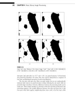
FIGURE 18.1
A three-level hierarchy wavelet decomposition of the 512 ϫ 512 color Lena image. Level 1
(512 ϫ 512) is the one-level wavelet representation of the original Lena at Level 0; Level 2
(256 ϫ 256) shows the one-level wavelet representation of the lowpass image at Level 1; and
Level 3 (128 ϫ 128) gives the one-level wavelet representation of the lowpass image at Level 2.
18.1 What Are Wavelets: Why Are They Good for Image Coding? 465
FIGURE 18.2
A three-level wavelet representation of the Lena image generated from the top view of the three-
level hierarchy wavelet decomposition in Fig. 18.1. It has exactly the same number of samples
as in the image domain.
in image compression. More importantly, our goal is to provide a high-level explanation
for why they are well suited for image compression. Indeed, wavelets have superior
properties vis-a-vis the more traditional Fourier-based method in the form of the discrete
cosine transform (DCT) that is deployed in the old JPEG image compression standard
(see Chapter 17). We will also cover powerful generalizations of wavelets, known as
wavelet packets, that have already made an impact in the standardization world: the FBI
fingerprint compression standard is based on wavelet packets.
Although this chapter is about image coding,
1
which involves two-dimensional (2D)

signals or images, it is much easier to understand the role of wavelets in image coding
using a one-dimensional (1D) framework, as the conceptual extension to 2D is straight-
forward. In the interests of clarity, we will therefore consider a 1D treatment here. The
story begins with what is known as the time-frequency analysis of the 1D signal. As
mentioned, wavelets are a tool for chang ing the coordinate system in which we represent
the signal: we transform the signal into another domain that is much better suited for
processing, e.g., compression. What makes for a good transform or analysis tool? At the
basic level, the goal is to be able to represent all the useful signal features and impor tant
phenomena in as compact a manner as possible. It is important to be able to compact the
bulk of the signal energy into the fewest number of transform coefficients: this way, we
can discard the bulk of the transform domain data without losing too much information.
For example, if the signal is a time impulse, then the best thing is to do no transforms at
1
We use the terms image compression and image coding interchangeably in this chapter.
466 CHAPTER 18 Wavelet Image Compression
all! Keep the signal information in its original and sparse time-domain representation,
as that will maximize the temporal energy concentration or time resolution. However,
what if the signal has a critical frequency component (e.g., a low-frequency background
sinusoid) that lasts for a long t ime duration? In this case, the energy is spread out in
the time domain, but it would be succinctly captured in a single frequency coefficient if
one did a Fourier analysis of the signal. If we know that the signals of interest are pure
sinusoids, then Fourier analysis is the way to go. But, what if we want to capture both
the time impulse and the frequency impulse with good resolution? Can we get arbitrarily
fine resolution in both time and frequency?
The answer is no. There exists an uncertainty theorem (much like what we learn
in quantum physics), which disallows the existence of arbitrary resolution in time and
frequency [2]. A good way of conceptualizing these ideas and the role of wavelet basis
functions is through what is known as time-frequency“tiling”plots, as shown in Fig . 18.3,
which shows where the basis functions live on the time-frequency plane: i.e., where is
the bulk of the energy of the elementary basis elements localized? Consider the Fourier

Time
Frequency
(a)
Time
Frequency
(
b
)
FIGURE 18.3
Tiling diagrams associated with the STFT bases and wavelet bases. (a) STFT bases and the tiling
diagram associated with a STFT expansion. STFT bases of different frequencies have the same
resolution (or length) in time; (b) Wavelet bases and tiling diagram associated with a wavelet
expansion. The time resolution is inversely proportional to frequency for wavelet bases.
18.1 What Are Wavelets: Why Are They Good for Image Coding? 467
case first. As impulses in time are completely spread out in the frequency domain, all
localization is lost with Fourier analysis. To alleviate this problem, one typically decom-
poses the signal into finite-length chunks using windows or so-called short-time Fourier
transform (STFT). Then, the time-frequency tradeoffs will be determined by the win-
dow size. An STFT expansion consists of basis functions that are shifted versions of
one another in both time and frequency: some elements capture low-frequency events
localized in time, and others capture high-frequency events localized in time, but the
resolution or window size is constant in both time and frequency (see Fig. 18.3(a)). Note
that the uncertainty theorem says that the area of these tiles has to be nonzero.
Shown in Fig. 18.3(b) is the corresponding tiling diagram associated with the wavelet
expansion. The key difference between this and the Fourier case, which is the critical
point, is that the tiles are not all of the same size in time (or frequency). Some basis
elements have short time windows; others have short frequency windows. Of course, the
uncertainty theorem ensures that the area of each tile is constant and nonzero. It can be
shown that the basis functions are related to one another by shifts and scales as this is the
key to wavelet analysis.

Why are wavelets well suited for image compression? The answer lies in the time-
frequency (or more correctly, space-frequency) characteristics of typical natural images,
which turn out to be well captured by the wavelet basis functions shown in Fig. 18.3(b).
Note that the STFT tiling diagram of Fig. 18.3(a) is conceptually similar to what com-
mercial DCT-based image transform coding methods like JPEG use. Why are wavelets
inherently a better choice? Looking at Fig . 18.3(b), one can note that the wavelet basis
offers elements having good frequency resolution at lower frequency (the short and fat
basis elements) while simultaneously offering elements that have good time resolution at
higher frequencies (the tall and skinny basis elements).
This tradeoff works well for natural images and scenes that are t ypically composed of
a mixture of important long-term low-frequency trends that have larger spatial duration
(such as slowly varying backgrounds like the blue sky, and the surface of lakes) as well
as important transient short duration high-frequency phenomena such as sharp edges.
The wavelet representation turns out to be par ticularly well suited to capturing both
the transient high-frequency phenomena such as image edges (using the tall and skinny
tiles) and long spatial duration low-frequency phenomena such as image backgrounds
(the short and fat tiles). As natural images are dominated by a mixture of these kinds of
events,
2
wavelets promise to be very efficient in capturing the bulk of the image energy
in a small fraction of the coefficients.
To summarize, the task of separating transient behavior from long-term trends is a
very difficult task in image analysis and compression. In the case of images, the difficulty
stems from the fact that statistical analysis methods often require the introduction of at
least some local stationarity assumption, i.e., the image statistics do not change abruptly
2
Typical images also contain textures; however, conceptually, textures can be assumed to be a dense
concentration of edges, and so it is fairly accurate to model typical images as smooth regions delimited
by edges.
468 CHAPTER 18 Wavelet Image Compression

over time. In practice, this assumption usually translates into ad hoc methods to block
data samples for analysis, methods that can potentially obscure important signal features:
e.g., if a block is chosen too big, a transient component might be totally neglected when
computing averages. The blocking artifact in JPEG decoded images at low rates is a result
of the block-based DCT approach. A fundamental contribution of wavelet theory [3] is
that it provides a unified framework in which transients and trends can be simultaneously
analyzed without the need to resort to blocking methods.
As a way of highlighting the benefits of having a sparse representation, such as that
provided by the wavelet decomposition, consider the lowest frequency band in the top
level (Level 3) of the three-level wavelet hierarchy of Lena in Fig. 18.1. This band is just
a downsampled (by a factor of 8
2
ϭ 64) and smoothed version of the original image.
A ver y simple way of achieving compression is to simply retain this lowpass version and
throw away the rest of the wavelet data, instantly achieving a compression ratio of 64:1.
Note that if we want a full-size approximation to the original, we would have to inter-
polate the lowpass band by a factor of 64—this can be done efficiently by using a three-
stage synthesis filter bank (see Chapter 6). We may also desire better image fidelity, as
we may be compromising high-frequency image detail, especially perceptually important
high-frequency edge information. This is where wavelets are particularly attractive as they
are capableof capturing most imageinformation in the highly subsampled l ow-frequency
band and additional localized edge information in spatial clusters of coefficients in the
high-frequency bands (see Fig. 18.1). The bulk of the wavelet data is insignificant and
can be discarded or quantized very coarsely.
Another attractive aspect of the coarse-to-fine nature of the wavelet representation
naturally facilitates a transmission scheme that progressively refines the received image
quality. That is, it would be hig hly beneficial to have an encoded bitstream that can
be chopped off at any desired point to provide a commensurate reconstruction image
quality. This is known as a progressive transmission feature or as an embedded bitstream
(see Fig. 18.4). Many modern wavelet image coders have this feature, as will be covered

in more detail in Section 18.5. This is ideally suited, for example, to Internet image
applications. As is well known, the Internet is a heterogeneous mess in terms of the
number of users and their computational capabilities and effective bandwidths. Wavelets
provide a natural way to satisfy users having disparate bandwidth and computational
capabilities: the low-end users can be provided a coarse quality approximation, whereas
higher-end users can use their increased bandwidth to get better fidelity. This is also very
useful for Web browsing applications, where having a coarse quality image with a short
waiting time may be preferable to having a detailed quality with an unacceptable delay.
These are some of the high-level reasons why wavelets represent a superior alternative
to traditional Fourier-based methods for compressing natural images: this is why the
JPEG2000 standard [1] uses wavelets instead of the Fourier-based DCT.
In this chapter, we will review the salient aspects of the general compression prob-
lem and the transform coding paradigm in particular, and highlight the key differences
between the class of early subband coders and the recent more advanced class of modern-
day wavelet image coders. We pick the celebrated embedded zerotree wavelet (EZW)
coder as a representative of this latter class, and we describe its operation by using a
18.2 The Compression Problem 469
D
S3
D
S1
D
S2
Progressive encoder
Image
Encoded bitstream
01010001001101001100001010 10010100101100111010010010011 010010111010101011001010101
FIGURE 18.4
Multiresolution wavelet image representation naturally facilitates progressive transmission—
a desirable feature for the transmission of compressed images over heterogeneous packet

networks and wireless channels.
simple illustrative example. We conclude with more powerful generalizations of the basic
wavelet image coding framework to wavelet packets, which are particularly well suited to
handle special classes of images such as fingerprints.
18.2 THE COMPRESSION PROBLEM
Image compression falls under the general umbrella of data compression, which has been
studied theoretically in the field of information theory [4], pioneered by Claude Shannon
[5] in 1948. Information theory sets the fundamental bounds on compression perfor-
mance theoretically attainable for certain classes of sources. This is very useful because
it provides a theoretical benchmark against which one can compare the performance of
more pr actical but suboptimal coding algorithms.
470 CHAPTER 18 Wavelet Image Compression
Historically, the lossless compression problem came first. Here the goal is to compress
the source with no loss of information. Shannon showed that given any discrete source
with a well-defined statistical characterization (i.e., a probability mass function), there is
a fundamental theoretical limit to how well you can compress the source before you start
to lose information. This limit is called the entropy of the source. In lay terms, entropy
refers to the uncertainty of the source. For example, a source that takes on any of N
discrete values a
1
,a
2
, ,a
N
with equal probability has an entropy g iven by log
2
N bits
per source symbol. If the symbols are not equally likely, however, then one can do better
because more predictable symbols should be assigned fewer bits. The fundamental limit
is the Shannon entropy of the source.

Lossless compression of images has been covered in Chapter 16. For image coding,
typical lossless compression ratios are of the order of 2:1 or at most 3:1. For a 512 ϫ 512
8-bit grayscale image, the uncompressed representation is 256 Kbytes. Lossless compres-
sion would reduce this to at best ∼80 Kbytes, which may still be excessive for many
practical low-bandwidth transmission applications. Furthermore, lossless image com-
pression is for the most part overkill, as our human vi sual system is highly tolerant to
losses in visual information. For compression ratios in the range of 10:1 to 40:1 or more,
lossless compression cannot do the job, and one needs to resort to lossy compression
methods.
The formulation of the lossy data compression framework was also pioneered by
Shannon in his work on rate-distortion (RD) theory [6], in which he formalized the
theory of compressing certain limited classes of sources having well-defined statistical
properties, e.g., independent, identically distributed (i.i.d.) sources having a Gaussian
distribution subject to a fidelity criterion, i.e., subject to a tolerance on the maximum
allowable loss or distortion that can be endured. Typical distortion measures used are
mean square error (MSE) or peak signal-to-noise ratio (PSNR)
3
between the original and
compressed versions. These fundamental compression performance bounds are called
the theoretical RD bounds for the source: they dictate the minimum rate R needed to
compress the source if the tolerable distortion level is D (or alternatively, what is the
minimum distortion D subjecttoabitrateofR). These bounds are unfortunately not
constructive; i.e., Shannon did not give an actual algorithm for attaining these bounds,
and furthermore, they are based on arguments that assume infinite complexity and delay,
obviously impractical in real life. However, these bounds are useful in as much as they
provide valuable benchmarks for assessing the performance of more practical coding
algorithms. The major obstacle of course, as in the lossless case, is that these theoretical
bounds are available only for a nar row class of sources, and it is difficult to make the
connection to real world image sources which are difficult to model accurately with
simplistic statistical models.

Shannon’s theoretical RD framework has inspired the design of more pr actical
operational RD frameworks, in which the goal is similar but the framework is con-
strained to be more practical. Within the operational constraints of the chosen coding
3
The PSNR is defined as 10 log
10
255
2
MSE
and measured in decibels (dB).
18.3 The Transform Coding Paradigm 471
framework, the goal of operational RD theory is to minimize the rate R subject to a
distortion constraint D, or vice versa. The message of Shannon’s RD theory is that one
can come close to the theoretical compression limit of the source if one considers vectors
of source symbols that get infinitely large in dimension in the limit; i.e., it is a good
idea not to code the source symbols one at a time, but to consider chunks of them at
a time, and the bigger the chunks the better. This thinking has spawned an impor tant
field known as vector quantization (VQ) [7], which, as the name indicates, is concerned
with the theory and practice of quantizing sources using high-dimensional VQ. There
are practical difficulties arising from making these vectors too high-dimensional because
of complexity constraints, so practical frameworks involve relatively small dimensional
vectors that are therefore further from the theoretical bound.
Due to this difficulty, there has been a much more popular image compression frame-
work that has taken off in practice: this is the transform coding framework [8] that forms
the basis of current commercial image and video compression standards like JPEG and
MPEG (see Chapters 9 and 10 in [9]). The transform coding paradigm can be construed
as a practical special case of VQ that can attain the promised gains of processing source
symbols in vectors through the use of efficiently implemented high dimensional source
transforms.
18.3 THE TRANSFORM CODING PARADIGM

In a typical transform image coding system, the encoder consists of a linear transform
operation, followed by quantization of transform coefficients, and lossless compression
of the quantized coefficients using an entropy coder. After the encoded bitstream of an
input image is transmitted over the channel (assumed to be perfect), the decoder undoes
all the functionalities applied in the encoder and tries to reconstruct a decoded image
that looks as close as possible to the original input image, based on the transmitted
information. A block diagram of this transform image paradigm is shown in Fig. 18.5.
For the sake of simplicity, let us look at a 1D example of how transform coding is
done (for 2D images, we treat the rows and columns separately as 1D signals). Suppose
we have a two-point signal, x
0
ϭ 216, x
1
ϭ 217. It takes 16 bits (8 bits for each sample)
to store this signal in a computer. In transform coding, we first put x
0
and x
1
in a column
vector X ϭ

x
0
x
1

and apply an orthogonal transformation T to X to get Y ϭ

y
0

y
1

ϭ
TX ϭ

1/
√
21/
√
2
1/
√
2 Ϫ1/
√
2

x
0
x
1

ϭ

(x
0
ϩ x
1
)/
√

2
(x
0
Ϫ x
1
)/
√
2

ϭ

306.177
Ϫ.707

. The transform T can
be conceptualized as a counter-clockwise rotation of the signal vector X by 45
◦
with
respect to the original (x
0
, x
1
) coordinate system. Alternatively and more conveniently,
one can think of the signal vector as being fixed and instead rotate the (x
0
, x
1
) coordinate
system by 45
◦

clockwise to the new (y
1
, y
0
) coordinate system (see Fig. 18.6). Note that
the abscissa for the new coordinate system is now y
1
.
Orthogonality of the transform simply means that the length of Y is the same as
the length of X (which is even more obvious when one freezes the signal vector and
472 CHAPTER 18 Wavelet Image Compression
(b)
(a)
Linear
transform
Quantization
Entropy
coding
010111
0.5 b/p
Original
image
Inverse
transform
010111
Entropy
decoding
Decoded
image
Inverse

quantization
FIGURE 18.5
Block diagrams of a typical transform image coding system: (a) encoder and (b) decoder
diagrams.
x
1
x
0
0
216
217
306.177
20.707
X
y
1
y
0
FIGURE 18.6
The transform T can be conceptualized as a counter-clockwise rotation of the signal vector X
by 45
◦
with respect to the original (x
0
, x
1
) coordinate system.
rotates the coordinate system as discussed above). This concept still carries over to the
case of high-dimensional transforms. If we decide to use the simplest form of quanti-
zation known as uniform scalar quantization, where we round off a real number to the

nearest integer multiple of a step size q (say q ϭ 20), then the quantizer index vector
ˆ
I,
which captures what integer multiples of q are nearest to the entries of Y ,isgivenby
18.3 The Transform Coding Paradigm 473
ˆ
I ϭ

round(y
0
/q)
round(y
1
/q)

ϭ

15
0

. We store (or transmit)
ˆ
I as the compressed version of X
using 4 bits, achieving a compression ratio of 4:1. To decode X from
ˆ
I, we first multi-
ply
ˆ
I by q ϭ 20 to dequantize, i.e., to form the quantized approximation
ˆ

Y of Y with
ˆ
Y ϭ q ·
ˆ
I ϭ

300
0

, andthen apply theinverse transform T
Ϫ1
to
ˆ
Y (which corresponds in
our example to a counter-clockwise rotation of the (y
1
,y
0
) coordinate system by 45
◦
, just
the reverse operation of the T operation on the original (x
0
,x
1
) coordinate system—see
Fig. 18.6)toget
ˆ
X ϭ T
Ϫ1


qy
0
qy
1

ϭ

1/
√
21/
√
2
1/
√
2 Ϫ1/
√
2

300
0

ϭ

212.132
212.132

.
We see from the above example that, although we “zero out” or throw away the
transform coefficient y

1
in quantization, the decoded version
ˆ
X is still very close to X.
This is because the transform effectively compacts most of the energy in X into the first
coefficient y
0
, and renders the second coefficient y
1
considerably insignificant to keep.
The transform T in our example actually computes a weighted sum and difference of
the two samples x
0
and x
1
in a manner that preserves the original energy. It is in fact the
simplest wavelet transform!
The energy compaction aspect of wavelet transforms was highlighted in Section 18.1.
Another goal of linear transformation is decorrelation. This can be seen from the fact
that, although the values of x
0
and x
1
are very close (highly correlated) before the trans-
form, y
0
(sum) and y
1
(difference) are very different (less correlated) after the transform.
Decorrelation has a nice geometric interpretation. A cloud of input samples of length-2

is shown along the 45
◦
line in Fig. 18.7. The coordinates (x
0
,x
1
) at each point of the cloud
are nearly the same, reflecting the high degree of correlation among neighboring image
pixels. The linear transformation T essentially amounts to a rotation of the coordinate
FIGURE 18.7
Linear transformation amounts to a rotation of the coordinate system, making correlated samples
in the time domain less correlated in the transform domain.
474 CHAPTER 18 Wavelet Image Compression
system. The axes of the new coordinate system are parallel and perpendicular to the ori-
entation of the cloud. The coordinates (y
0
,y
1
) are less correlated, as their magnitudes can
be quite different and the sign of y
1
is random. If we assume x
0
and x
1
are samples
of a stationary random sequence X (n), then the correlation between y
0
and y
1

is
E{y
0
y
1
} ϭ E{(x
2
0
Ϫ x
2
1
)/2} ϭ 0. This decorrelation propert y has significance in terms
of how much gain one can get from transform coding than from doing signal process-
ing (quantization and coding) directly in the original signal domain, called pulse code
modulation (PCM) coding.
Transform coding has been extensively developed for coding of images and video,
where the DCT is commonly used because of its computational simplicity and its good
performance. But as shown in Section 18.1, the DCT is giving way to the wavelet trans-
form because of the latter’s superior energy compaction capability when applied to
natural images. Before discussing state-of-the-art wavelet coders and their advanced
features, we address the functional units that comprise a transform coding system,
namely the transform, quantizer, and entropy coder (see Fig. 18.5).
18.3.1 Transform Structure
The basic idea behind using a linear transformation is to make the task of compressing an
image in the t ransform domain after quantization easier than direct coding in the spatial
domain. Agood transform, as has been mentioned,should beable to decorrelate the image
pixels and provide good energy compaction in the transform domain so that very few
quantized nonzero coefficients have to be encoded. It is also desirable for the transform
to be orthogonal so that the energy is conserved from the spatial domain to the trans-
form domain, and the distortion in the spatial domain introduced by quantization of

transform coefficients can be directly examined in the transform domain. What makes
the wavelet transform special in all possible choices is that it offers an efficient space-
frequency characterization for a broad class of natural images, as shown in Section 18.1.
18.3.2 Quantization
As the only source of information loss occurs in the quantization unit, efficient quantizer
design is a key component in wavelet image coding. Quantizers come in many differ-
ent shapes and forms, from very simple uniform scalar quantizers, such as the one in
the example earlier, to ver y complicated vector quantizers. Fixed length uniform scalar
quantizers are the simplest kind of quantizers: these simply round off real numbers to
the nearest integer multiples of a chosen step size. The quantizers are fixed length in the
sense that all quantization levels are assigned the same number of bits (e.g., an eight-level
quantizer would be assigned all binary three-tuples between 000 and 111). Fixed length
nonuniform scalar quantizers, in which the quantizer step sizes are not all the same, are
more powerful: one can optimize the design of these nonuniform step sizes to get what
is known as Lloyd-Max quantizers [10].
It is more efficient to do a joint design of the quantizer and the entropy coding func-
tional unit (this will be described in the next subsection) that follows the quantizer in
a lossy compression system. This joint design results in a so-called entropy-constrained
18.3 The Transform Coding Paradigm 475
quantizer that is more efficient but more complex, and results in variable length quan-
tizers in which the different quantization choices are assigned variable codelengths.
Variable length quantizers can come in either scalar, known as entropy-constrained
scalar quantization (ECSQ) [11], or vector varieties, known as entropy-constrained vec-
tor quantization (ECVQ) [7]. An efficient way of implementing vector quantizers is by
the use of so-called trellis coded quantization (TCQ) [12]. The performance of the quan-
tizer (in conjunction with the entropy coder) characterizes the operational RD function
of the source. The theoretical RD function characterizes the fundamental lossy compres-
sion limit theoretically attainable [13], and it is rarely known in analytical form except
for a few special cases, such as the i.i.d. Gaussian source [4]:
D(R) ϭ ␴

2
2
Ϫ2R
, (18.1)
where the Gaussian source is assumed to have zero mean and variance ␴
2
and the rate
R is measured in bits per sample. Note from the formula that every extra bit reduces
the expected distortion by a factor of 4 (or increases the signal to noise ratio by 6 dB).
This formula agrees with our intuition that the distortion should decrease exponentially
as the rate increases. In fact, this is true when quantizing sources with other probability
distributions as well under high-resolution (or bit rate) conditions: the optimal RD
performance of encoding a zero mean stationary source with variance ␴
2
takes the form
of [7]
D(R) ϭ h␴
2
2
Ϫ2R
, (18.2)
where the factor h depends on the probability distribution of the source. For a Gaussian
source, h ϭ
√
3␲/2 with optimal scalar quantization. Under high-resolution conditions,
it can be shown that the optimal entropy-constrained scalar quantizer is a uniform one,
whose average distortion is only approximately 1.53 dB worse than the theoretical bound
attainable that is known as the Shannon bound [7, 11]. For low bit rate coding, most
current subband coders employ a uniform quantizer with a “deadzone” in the central
quantization bin. This simply means that the all-important central bin is wider than

the other bins: this turns out to be more efficient than having all bins be of the same
size. The performance of deadzone quantizers is nearly optimal for memoryless sources
even at low rates [14]. An a dditional advantage of using deadzone quantization is that,
when the deadzone is twice as much as the uniform step size, an embedded bitstream can
be generated by successive quantization. We will elaborate more on embedded wavelet
image coding in Section 18.5.
18.3.3 Entropy Coding
Once the quantization process is completed, the last encoding step is to use entropy cod-
ing to achieve the entropy rate of the quantizer. Entropy coding works like the Morse
code in electric telegraph: more frequently occurring symbols are represented by short
codewords, whereas symbols occurring less frequently are represented by longer code-
words. On average, entropy coding does better than assigning the same codelength to
all symbols. For example, a source that can take on any of the four symbols {A,B, C,D}
476 CHAPTER 18 Wavelet Image Compression
with equal likelihood has 2 bits of information or uncertainty, and its entropy is 2 bits
per symbol (e.g., one can assig n a binary code of 00 to A,01toB,10toC, and 11 to D).
However if the symbols are not equally likely, e.g., if the probabilities of A, B,C, and D
are 0.5,0.25,0.125, and 0.125, respectively, then one can do much better on average by
not assigning the same number of bits to each symbol but rather by assigning fewer bits
to the more popular or predictable ones. This results in a variable length code. In fact,
one can show that the optimal code would be one in which A gets 1 bit, B gets 2 bits, and
C and D get 3 bits each (e.g., A ϭ 0,B ϭ 10, C ϭ 110, and D ϭ 111). This is called an
entropy code. With this code, one can compress the source with an average of only 1.75
bits per symbol, a 12.5% improvement in compression over the original 2 bits per sym-
bol associated with having fixed length codes for the symbols. The two popular entropy
coding methods are Huffman coding [15] and arithmetic coding [16]. A comprehensive
coverage of entropy coding is give n in Chapter 16. The Shannon entropy [4] provides a
lower bound in terms of the amount of compression entropy coding can best achieve.
The optimal entropy code constructed in the example actually achieves the theoretical
Shannon entropy of the source.

18.4 SUBBAND CODING: THE EARLY DAYS
Subband coding nor mally uses bases of roughly equal bandwidth. Wavelet image coding
can be viewed as aspecial case of subband coding with logarithmically varying bandwidth
bases that satisfy certain properties.
4
Early work on wavelet image coding was thus hidden
under the name of subband coding [8, 17], which builds upon the traditional transform
coding paradigm of energ y compaction and decorrelation. The main idea of subband
coding is to treat different bands differently as each band can be modeled as a statistically
distinct process in quantization and coding.
To illustrate the design philosophy of early subband coders, let us again assume, for
example, that we are coding a vector source {x
0
,x
1
}, where both x
0
and x
1
are samples of
a stationary random sequence X(n) with zero mean and variance ␴
2
x
.Ifwecodex
0
and
x
1
directly by using PCM coding, from our earlier discussion on quantization, the RD
performance can be approximated as

D
PCM
(R) ϭ h␴
2
x
2
Ϫ2R
. (18.3)
In subband coding, two quantizers are designed: one for each of the two transform
coefficients y
0
and y
1
. The goal is to choose rates R
0
and R
1
needed for coding y
0
and y
1
so that the average distortion
D
SBC
(R) ϭ (D(R
0
) ϩ D(R
1
))/2 (18.4)
is minimized with the constraint on the average bit rate

(R
0
ϩ R
1
)/2 ϭ R. (18.5)
4
Both wavelet image coding and subband coding are special cases of transform coding.
18.4 Subband Coding: The Early Days 477
Using the high rate approximation, we write D(R
0
) ϭ h ␴
2
y
0
2
Ϫ2R
0
and D(R
1
) ϭ
h␴
2
y
1
2
Ϫ2R
1
; then the solutions to this bit allocation problem are [8]
R
0

ϭ R ϩ
1
2
log
2
␴
y
0
␴
y
1
; R
1
ϭ R Ϫ
1
2
log
2
␴
y
0
␴
y
1
, (18.6)
with the minimum average distortion being
D
SBC
(R) ϭ h␴
y

0
␴
y
1
2
Ϫ2R
. (18.7)
Note that, at the optimal point, D(R
0
) ϭ D(R
1
) ϭ D
SBC
(R). That is, the quantizers
for y
0
and y
1
give the same distortion with optimal bit allocation. Since the transform
T is orthogonal, we have ␴
2
x
ϭ (␴
2
y
0
ϩ ␴
2
y
1

)/2. The coding gain of using subband coding
over PCM is
D
PCM
(R)
D
SBC
(R)
ϭ
␴
2
x
␴
y
0
␴
y
1
ϭ
(␴
2
y
0
ϩ ␴
2
y
1
)/2
(␴
2

y
0
␴
2
y
1
)
1/2
, (18.8)
the ratio of arithmetic mean to geometric mean of coefficient variances ␴
2
y
0
and ␴
2
y
1
. What
this important result states is that subband coding performs no worse than PCM coding ,
and that the larger the disparity between coefficient variances, the bigger the subband
coding gain, because (␴
2
y
0
ϩ ␴
2
y
1
)/2 Ն (␴
2

y
0
␴
2
y
1
)
1/2
, with equality if ␴
2
y
0
ϭ ␴
2
y
1
. This result
can be easily extended to the case when M > 2 uniform subbands (of equal size) are used
instead. The coding gain in this general case is as follows:
D
PCM
(R)
D
SBC
(R)
ϭ
1
M

MϪ1

kϭ0
␴
2
k


MϪ1
kϭ0
␴
2
k

1/M
, (18.9)
where ␴
2
k
is the sample variance of the kth band (0 Յ k Յ M Ϫ 1). The above assumes
that all M bands are of the same size. In the case of the subband or wavelet transform,
the sizes of the subbands are not the same (see Fig. 18.8), but the above formula can be
generalized pretty easily to account for this. As another extension of the results given in
the above example, it can be shown that the necessary condition for optimal bit allocation
is that all subbands should incur the same distortion at optimality—else it is possible to
steal some bits from the lower distortion bands to the higher distortion bands in a way
that makes the overall performance better.
Figure 18.8 shows typical bit allocation results for different subbands under a total
bit rate budget of 1 bit per pixel for wavelet image coding. Since low-frequency bands in
the upper-left corner have far more energy than high-frequency bands in the lower-right
corner (see Fig. 18.1), more bits have to be allocated to lowpass bands than to highpass
bands. The last two frequency bands in the bottom half are not coded (set to zero)

because of limited bit rate. Since subband coding t reats wavelet coefficients according to
their frequency bands, it is effectively a frequency domain transform technique.
Initial wavelet-based coding algorithms, e.g., [18], followed exactly this subband cod-
ing methodology. These algorithms were designed to exploit the energy compaction
478 CHAPTER 18 Wavelet Image Compression
86
55
2
22
1
00
FIGURE 18.8
Typical bit allocation results for different subbands. The unit of the numbers is bits per pixel.
These are designed to satisfy a total bit rate budget of 1 bit per pixel. That is, {[(8 ϩ 6 ϩ 5 ϩ
5)/4 ϩ 2 ϩ 2 ϩ 2]/4 ϩ 1 ϩ 0ϩ 0}/4 ϭ 1.
properties of the wavelet transform only in the frequency domain by applying quantizers
optimized for the statistics of each frequency band. Such algorithms have demonstrated
small improvements in coding efficiency over standard transform-based algorithms.
18.5 NEW AND MORE EFFICIENT CLASS OF WAVELET CODERS
Because wavelet decompositions offer space-frequency representations of images, i.e.,
low-frequency coefficients have large spatial support (good for representing large image
background regions), whereas high-frequency coefficients have small spatial support
(good for representing spatially local phenomena such as edges), the wavelet represen-
tation calls for new quantization strategies that go beyond traditional subband coding
techniques to exploit this underlying space-frequency image characterization.
Shapiro made a breakthrough in 1993 with his EZW coding algorithm [19]. Since
then a new class of algorithms have been developed that achieve significantly improved
performance over the EZW coder. In particular, Said and Pearlman’s work on set parti-
tioning inhierarchical trees (SPIHT) [20],which improves theEZW coder, has established
zerotree techniques as the current state-of-the-art of wavelet image coding since the

SPIHT algorithm proves to be very successful for both lossy and lossless compression.
18.5.1 Zerotree-Based Framework and EZW Coding
A wavelet image representation can be thought of as a tree-structured spatial set of
coefficients. A wavelet coefficient tree is defined as the set of coefficients from different
bands that represent the same spatial region in the image. Figure 18.9 shows a three-
level wavelet decomposition of the Lena image, together with a wavelet coefficient tree
18.5 New and More Efficient Class of Wavelet Coders 479
(a) (b)
HL
2
HL
3
LH
1
LH
2
LH
3
HH
2
HH
3
HL
1
HH
1
FIGURE 18.9
Wavelet decomposition offers a tree-structured image representation. (a) Three-level wavelet
decomposition of the Lena image; (b) Spatial wavelet coefficient tree consisting of coefficients
from different bands that correspond to the same spatial region of the original image (e.g., the

eye of Lena). Arrows identify the parent-children dependencies.
structure representing the eye region of Lena.ArrowsinFig. 18.9(b) identify the parent-
children dependencies in a tree. The lowest frequency band of the decomposition is
represented by the root nodes (top) of the tree, the highest frequency bands by the
leaf nodes (bottom) of the tree, and each parent node represents a lower frequency
component than its children. Except for a root node, which has only three children
nodes, each parent node has four children nodes, the 2 ϫ 2 region of the same spatial
location in the immediately higher frequency band.
Both the EZW and SPIHT algorithms [19, 20] are based on the idea of using multipass
zerotree coding to transmit the largest wavelet coefficients (in magnitude) at first. We
hereby use “zero coding” as a generic term for both schemes, but we focus on the popular
SPIHT coder because of its superior performance. A set of tree coefficients is significant
if the largest coefficient magnitude in the set is greater than or equal to a certain threshold
(e.g., a power of 2); otherwise, it is insignificant. Similarly, a coefficient is significant if its
magnitude is greater than or equal to the threshold; otherwise, it is insignificant. In each
pass the significance of a larger set in the t ree is tested at first: if the set is insignificant, a
binary “zerotree” bit is used to set all coefficients in the set to zero; otherwise, the set is
partitioned into subsets (or child sets) for further significance tests. After all coefficients
are tested in one pass, the threshold is halved before the next pass.
The underlying assumption of the zerotree coding framework is that most images
can be modeled as having decaying power spectral densities. That is, if a parent node in
the wavelet coefficient tree is insignificant, it is very likely that its descendents are also
480 CHAPTER 18 Wavelet Image Compression
23463 49
213 14
10 7 13 212 7
3 4 621
15 14 3 212 5 27 3 9
214 8 4 22 3 2
9 2147 4 622 2

30232 322 0 4
2 23624 3 6 36
511 5 6 0 324 4
29 27
231
25
23
FIGURE 18.10
Example of a three-level wavelet representation of an 8 ϫ 8 image.
insignificant. The zerotree symbol is used very efficiently in this case to signify a spatial
subtree of zeros.
We give a SPIHT coding example to highlight the order of operations in zerotree
coding. Start with a simple three-level wavelet representation of an 8 ϫ 8 image,
5
as
shown in Fig. 18.10. The largest coefficient magnitude is 63. We can choose a threshold
in the first pass between 31.5 and 63. Let T
1
ϭ 32. Table 18.1 shows the first pass of the
SPIHT coding process, with the following comments:
1. The coefficient value 63 is greater than the threshold 32 and positive, so a sig-
nificance bit “1” is generated, followed by a positive sign bit “0.” After decoding
these symbols, the decoder knows the coefficient is between 32 and 64 and uses
the midpoint 48 as an estimate.
6
2. The descendant set of coefficient Ϫ34 is significant; a significance bit “1” is
generated, followed by a significance test of each of its four children {49,10,
14,Ϫ13}.
3. The descendant set of coefficient Ϫ31 is significant; a significance bit “1” is gen-
erated, followed by a significance test of each of its four children {15, 14,Ϫ9,Ϫ7}.

5
This set of wavelet coefficients is the same as the one used by Shapiro in an example to showcase EZW
coding [19]. Curious readers can compare these two examples to see the difference between EZW and
SPIHT coding.
6
The reconstruction value can be anywhere in the uncertainty interval (32,64). Choosing the midpoint is
the result of a simple form of minimax estimation.
18.5 New and More Efficient Class of Wavelet Coders 481
TABLE 18.1 First pass of the SPIHT coding process at threshold T
1
ϭ 32.
Coefficient Coefficient Binary Reconstruction
coordinates value symbol value Comments
(0,0) 63 1 (1)
048
(1,0) Ϫ34 1
1 Ϫ48
(0,1) Ϫ31 0 0
(1,1) 23 0 0
(1,0) Ϫ34 1 (2)
(2,0) 49 1
048
(3,0) 10 0 0
(2,1) 14 0 0
(3,1) Ϫ13 0 0
(0,1) Ϫ31 1 (3)
(0,2) 15 0 0
(1,2) 14 0 0
(0,3) Ϫ90 0
(1,3) Ϫ70 0

(1,1) 23 0 (4)
(1,0) Ϫ34 0 (5)
(0,1) Ϫ31 1 (6)
(0,2) 15 0 (7)
(1,2) 14 1 (8)
(2,4) Ϫ10 0
(3,4) 47 1
048
(2,5) Ϫ30 0
(3,5) 2 0 0
(0,3) Ϫ9 0 (9)
(1,3) Ϫ70
4. The descendant set of coefficient 23 is insignificant; an insignificance bit “0” is
generated. This zerotree bit is the only symbol generated in the current pass for
the whole descendant set of coefficient 23.
5. The grandchild set of coefficient Ϫ34 is insignificant; a binary bit“0”is generated.
7
7
In this example, we use the following convention: when a coefficient or set is significant, a binary bit “1” is
generated; otherwise, a binary bit “0” is generated. In the actual SPIHT implementation [20], this conven-
tion was not always followed—when a grandchild set is significant, a binary bit “0” is generated, otherwise,
a binary bit “1” is generated.
482 CHAPTER 18 Wavelet Image Compression
6. The grandchild set of coefficient Ϫ31 is significant; a binary bit “1” is generated.
7. The descendant set of coefficient 15 is insignificant; an insignificance bit “0” is
generated. This zerotree bit is the only symbol generated in the current pass for
the whole descendant set of coefficient 15.
8. The descendant set of coefficient 14 is significant; a significance bit“1”is generated,
followed by a significance test of each of its four children {Ϫ1,47,Ϫ3,2}.
9. Coefficient Ϫ31 has four children {15,14,Ϫ9,Ϫ7}. Descendant sets of child 15and

child 14 were tested for significance before. Now descendant sets of the remaining
two children Ϫ9 and Ϫ7 are tested.
In this example, the encoder generates 29 bits in the first pass. Along the process,
it identifies four significant coefficients {63,Ϫ34,49,47}. The decoder reconstructs each
coefficient based on these bits. When a set is insignificant, the decoder knows each
coefficient in the set is between Ϫ32 and 32 and uses the midpoint 0 as an estimate. The
reconstruction result at the end of the first pass is shown in Fig. 18.11(a).
The threshold is halved (T
2
ϭ T
1
/2 ϭ 16) before the second pass, where insignificant
coefficients and sets in the first pass are tested for significance again against T
2
, and
significant coefficients found in the first pass are refined. The second pass thus consists
of the following:
1. Significance tests of the 12 insignificant coefficients found in the first pass—those
having reconstruction value 0 in Table 18.1. Coefficients Ϫ31 at (0, 1) and 23 at
(1, 1) are found to be significant in this pass; a sign bit is generated for each. The
48
0 0
0 0 0 0 0
0 0 0
0 0 0 0 0 0
0 0 0 0
048 0 0 0
0 0 0 0 0 0
0 0 0 0 0
0 0 0 0 0 0

0
0
0
0
0
0
0
0 0
0
0
0
0 0
0
0
0
0 0
248 48
(a)
0
0 0 0 0 0
0 0 0
0 0 0 0 0 0
0 0 0 0
0 0 0 0
0 0 0 0 0 0
0 0 0 0 0
0 0 0 0 0 0
0
0
0

0
0
0
0
0 0
0
0
0
0 0
0
0
0 0
56 240 56
224 24
40
(b)
FIGURE 18.11
Reconstructions after the (a) first and (b) second passes in SPIHT coding.