The Essential Guide to Image Processing- P18 ppsx

19.5 Approaches for Color and Multispectral Images 519
(a) (b)
(c) (d)
FIGURE 19.10
Canny edge detector of Eq. (19.22) applied after Gaussian smoothing over a range of ␴:
(a) ␴ ϭ 0.5; (b) ␴ ϭ 1; (c) ␴ ϭ 2; and (d) ␴ ϭ 4. The thresholds are fixed in each case at T
U
ϭ 10
and T
L
ϭ 4.
only computational cost beyond that for grayscale images is incurred in obtaining the
luminance component image, if necessary. In many color spaces, such as YIQ, HSL,
CIELUV , and CIELAB, the luminance image is simply one of the components in that
representation. For others, such as RGB, computing the luminance image is usually easy
and efficient. The main drawback to luminance-only processing is that important edges
are often not confined to the luminance component. Therefore, a gray level difference in
the luminance component is often not the most appropriate criterion for edge detection
in color images.
520 CHAPTER 19 Gradient and Laplacian Edge Detection
(a) (b)
(c) (d)
FIGURE 19.11
Canny edge detector of Eq. (19.22) applied after Gaussian smoothing with ␴ ϭ 2: (a) T
U
ϭ 10,
T
L
ϭ 1; (b) T
U
ϭ T

L
ϭ 10; (c) T
U
ϭ 20, T
L
ϭ 1; (d) T
U
ϭ T
L
ϭ 20.AsT
L
is changed, notice the
effect on the results of hysteresis thresholding.
Another rather obvious approach is to apply a desired edge detection method sep-
arately to each color component and construct a cumulative edge map. One possibility
for overall gradient magnitude, shown here for the RGB color space, combines the
component gradient magnitudes [24]:


ٌf
c
(x,y)


ϭ


ٌf
R
(x,y)



ϩ


ٌf
G
(x,y)


ϩ


ٌf
B
(x,y)


.
The results, however, are biased according to the properties of the particular color space
used. It is often important to employ a color space that is appropriate for the target
19.5 Approaches for Color and Multispectral Images 521
application. For example, edge detection that is intended to approximate the human
visual system’s behavior should utilize a color space having a perceptual basis, such as
CIELUV or perhaps HSL. Another complication is the fact that the components’gradient
vectors may not always be similarly oriented, making the search for local maxima of
|ٌf
c
| along the gradient direction more difficult. If a total gradient image were to be
computed by summing the color component gradient vectors, not just their magnitudes,

then inconsistent orientations of the component gradients could destructively interfere
and nullify some edges.
Vector approaches to color edge detection, while generally less computationally effi-
cient, tend to have better theoretical justification. Euclidean distance in color space
between the color vectors of a given pixel and its neighbors can be a good basis for
an edge detector [24]. For the RGB case, the magnitude of the vector gradient is as
follows:


ٌf
c
(x,y)


ϭ



ٌf
R
(x,y)


2
ϩ


ٌf
G
(x,y)



2
ϩ


ٌf
B
(x,y)


2
.
Trahanias and Venetsanopoulos [29] described the use of vector order statistics as the
basis for color edge detection. A later paper by Scharcanski and Venetsanopoulos [26]
furthered the concept. While not strictly founded on the gradient or Laplacian, their
techniques are effective and worth mention here because of their vector bases. The basic
idea is to look for changes in local vector statistics, particularly vector dispersion, to
indicate the presence of edges.
Multispectral images can have many components, complicating the edge detection
problem even further. Cebrián et al. [6] describe several methods that are useful for mul-
tispectral images having any number of components. Their description uses the second
directional derivative in the gradient direction as the basis for the edge detector, but other
types of detectors can be used instead. The components-average method forms a gray-
scale image by averaging all components, which have first been Gaussian-smoothed, and
then finds the edges in that image. The method generally works well because multispec-
tral images tend to have high correlation between components. However, it is possible
for edge information to diminish or vanish if the components destructively interfere.
Cumani [8] explored operators for computing the vector gradient and created an
edge detection approach based on combining the component gradients. A multispectral

contrast function is defined, and the image is searched for pixels having maximal direc-
tional contrast. Cumani’s method does not always detect edges present in the component
bands, but it better avoids the problem of destructive interference between bands.
The maximal gradient method constructs asingle g radient image from the component
images [6]. The overall gradient image’s magnitude and direction values at a given pixel
are those of the component having the greatest gradient magnitude at that pixel. Some
edges can be missed by the maximal gradient technique because they may be swamped
by differently oriented, stronger edges present in another band.
The method of combining component edge maps is the least efficient because an edge
map must first be computed for every band. On the positive side, this method is capable
of detecting any edge that is detectable in at least one component image. Combination
522 CHAPTER 19 Gradient and Laplacian Edge Detection
of component edge maps into a single result is made more difficult by the edge location
errors induced by Gaussian smoothing done in advance. The superimposed edges can
become smeared in width because of the accumulated uncertainty in edge localization.
A thinning step applied during the combination procedure can greatly reduce this edge
blurring problem.
19.6 SUMMARY
Gray level edge detection is most commonly performed by convolving an image, f , with
a filter that is somehow based on the idea of the derivative. Conceptually, edges can be
revealedby locating either thelocal extrema of the first derivative of f or the zero-crossings
of its second derivative. The gradient and the Laplacian are the primary derivative-based
functions used to construct such edge-detection filters. The gradient, ٌ, is a 2D extension
of the first derivative while the Laplacian, ٌ
2
,actsasa2Dsecondderivative.Avariety
of edge detection algorithms and techniques have been de veloped that are based on the
gradient or Laplacian in some way. Like any type of derivative-based filter, ones based on
these two functions tend to be very sensitive to noise. Edge location errors, false edges,
and broken or missing edge segments are often problems with edge detection applied to

noisy images. For gradient techniques, thresholding is a common way to suppress noise
and can be done adaptively for better results. Gaussian smoothing is also very helpful
for noise suppression, especially when second-derivative methods such as the Laplacian
are used. The Laplacian of Gaussian approach can also provide edge information over a
range of scales, helping to further improve detection accuracy and noise suppression as
well as providing clues that may be useful during subsequent processing.
Recent comparisons of various edge detectors have been made by Heath et al. [13]
and Bowyer et al. [4]. They have concluded that the subjective quality of the results of
various edge detectors applied to real images is quite dependent on the images themselves.
Thus, there is no single edge detector that produces a consistently best overall result.
Furthermore, they found it difficult to predict the best choice of edge detector for a given
situation.
REFERENCES
[1] D. H. Ballard and C. M. Brown, Computer Vision. Prentice-Hall, Englewood Cliffs, NJ, 1982.
[2] V. Berzins. Accuracy of Laplacian edge detectors. Comput. Vis. Graph. Image Process., 27:195–210,
1984.
[3] A. C. Bovik, T. S. Huang, and D. C. Munson, Jr. The effect of median filter ing on edge estimation
and detection. IEEE Trans. Pattern Anal. Mach. Intell., PAMI-9:181–194, 1987.
[4] K. Bowyer, C. Kranenburg,and S. Dougherty. Edge detectorevaluation using empirical ROC curves.
Comput. Vis. Image Underst., 84:77–103, 2001.
[5] J. Canny. A computational approach to edge detection. IEEE Trans. Pattern Anal. Mach. Intell.,
PAMI-8:679–698, 1986.
References 523
[6] M. Cebrián, M. Perez-Luque, and G. Cisneros. Edge detection alternatives for multispectral remote
sensing images. In Proceedings of the 8th Scandinavian Conference on Image Analysis, Vol. 2,
1047–1054. NOBIM-Norwegian Soc. Image Pross & Pattern Recognition, Tromso, Norway, 1993.
[7] J. S. Chen, A. Huertas, and G. Medioni. Very fast convolution with Laplacian-of-Gaussian masks.
In Proc. IEEE Comput. Soc. Conf. Comput. Vis. Pattern Recognit., 293–298. IEEE, New York, 1986.
[8] A. Cumani. Edge detection in multispectral images. Comput. Vis. Graph. Image Process. Graph.
Models Image Process., 53:40–51, 1991.

[9] L. Ding and A. Goshtasby. On the Canny edge detector. Pattern Recognit., 34:721–725, 2001.
[10] R. M. Haralick and L. G. Shapiro. Computer and Robot Vision, Vol. 1. Addison-Wesley, Reading,
MA, 1992.
[11] Q. Ji and R. M. Haralick. Efficient facet edge detection and quantitative performance evaluation.
Pattern Recognit., 35:689–700, 2002.
[12] R. C. Hardie and C. G. Boncelet. Gradient-based edge detection using nonlinear edge enhancing
prefilters. IEEE Trans. Image Process., 4:1572–1577, 1995.
[13] M. Heath, S. Sarkar, T. Sanocki, and K. Bowyer. Comparison of edge detectors, a methodology and
initial study. Comput. Vis. Image Underst., 69(1):38–54, 1998.
[14] A. Huertas and G. Medioni. Detection of intensity changes with subpixel accuracy using Laplacian-
Gaussian masks. IEEE Trans. Pattern. Anal. Mach. Intell., PAMI-8(5):651–664, 1986.
[15] S. R. Gunn. On the discrete representation of the Laplacian of Gaussian. Pattern Recognit., 32:
1463–1472, 1999.
[16] A. K. Jain. Fundamentals of Digital Image Processing. Prentice-Hall, Englewood Cliffs, NJ, 1989.
[17] J. S. Lim. Two-Dimensional Signal and Image Processing. Prentice-Hall, Englewood Cliffs, NJ, 1990.
[18] D. Marr. Vision. W. H. Freeman, New York, 1982.
[19] D. Marr and E. Hildreth. Theory of edge detection. Proc. R. Soc. Lond. B, 270:187–217, 1980.
[20] B. Mathieu, P. Melchior, A. Oustaloup,and Ch. Ceyral. Fractional differentiation for edge detection.
Signal Processing, 83:2421–2432, 2003.
[21] J. Merron and M. Brady. Isotropic gradient estimation. In Proc. IEEE Comput. Soc. Conf. Comput.
Vis. Pattern Recognit., 652–659. IEEE, New York, 1996.
[22] V. S. Nalwa and T. O. Binford. On detecting edges. IEEE Trans. Pattern. Anal. Mach. Intell., PAMI-
8(6):699–714, 1986.
[23] W. K. Pratt. Digital Image Processing, 2nd ed. Wiley, New York, 1991.
[24] S. J. Sangw ine and R. E. N. Horne, editors. The Colour Image Processing Handbook. Chapman and
Hall, London, 1998.
[25] S. Sarkar and K. L. Boyer. Optimal infinite impulse response zero crossing based edge detectors.
Comput. Vis. Graph. Image Process. Image Underst., 54(2):224–243, 1991.
[26] J. Scharcanski and A. N. Venetsanopoulos. Edge detection of color images using directional
operators. IEEE Trans. Circuits Syst. Video Technol., 7(2):397–401, 1997.

[27] P. Siohan, D. Pele, and V. Ouvrard. Two design techniques for 2-D FIR LoG filters. In M. Kunt,
editor, Proc. SPIE, Visual Communications and Image Processing, Vol. 1360, 970–981, 1990.
[28] V. Torre and T. A. Poggio. On edge detection. IEEE Trans. Pattern Anal. Mach. Intell., PAMI-
8(2):147–163, 1986.
524 CHAPTER 19 Gradient and Laplacian Edge Detection
[29] P. E. Trahanias and A. N. Venetsanopoulos. Color edge detection using vector order statistics. IEEE
Trans. Image Process., 2(2):259–264, 1993.
[30] A. P. Witkin. Scale-space filtering. In Proc. Int. Joint Conf. Artif. Intell., 1019–1022. William
Kaufmann Inc., Karlsruhe, Germany, 1983.
[31] D. Ziou and S. Wang. Isotropic processing for gradient estimation. In Proc. IEEE Comput. Soc. Conf.
Comput. Vis. Pattern Recognit., 660–665. IEEE, New York, 1996.
CHAPTER
20
Diffusion Partial Differential
Equations for Edge
Detection
Scott T. Acton
University of Virginia
20.1 INTRODUCTION AND MOTIVATION
20.1.1 Partial Differential Equations in Image and Video Processing
The collision of imag ing and differential equations makes sense. Without motion or
change of scene or changes within the scene, imaging is worthless. First, consider a static
environment—we would not need vision in this environment, as the components of the
scene are unchang ing. In a dynamic environment, however, vision becomes the most
valuable sense. Second, consider a constant-valued image with no internal changes or
edges. Such an image is devoid of value in the information-theoretic sense.
The need for imaging is based on the presence of change. The mechanism for change
in both time and space is described and governed by differential equations.
The partial differential equations (PDEs) of interest in this chapter enact diffusion.In
chemistry or heat transfer,diffusion is a process that equilibrates concentration differences

without creating or destroying mass. In image and video processing, we can consider the
mass to be the pixel intensities or the gradient magnitudes, for example.
These important differential equations are PDEs, since they contain partial derivatives
with respect to spatial coordinates and time. These equations, especially in the case
of anisotropic diffusion, are nonlinear PDEs since the diffusion coefficient is typically
nonlinear.
20.1.2 Edges and Anisotropic Diffusion
Sudden, sustained changes in image intensity are called edges. We know that the human
visual system makes extensive uses of edges to perform visual tasks such as object recog-
nition [1]. Humans can recognize complex 3D objects using only line drawing s or image
edge information. Similarly, the extraction of edges from digital imagery allows a valu-
able abstraction of information and a reduction in processing and storage costs. Most
525
526 CHAPTER 20 Diffusion Partial Differential Equations for Edge Detection
definitions of image edges involve some concept of feature scale. Edges are said to exist
at certain scales—edges from detail existing at fine scales and edges from the boundaries
of large objects existing at large scales. Furthermore, large-scale edges exist at fine scales,
leading to a notion of edge causality.
In order to locate edges of various scales within an image, it is desirable to have an
image operator that computes a scaled version of a particular image or frame in a video
sequence. This operator should preserve the position of such edges and facilitate the
extraction of the edge map through the scale space. The tool of isotropic diffusion, a
linear lowpass filtering process, is not able to preserve the position of important edges
through the scale space. Anisotropic diffusion, however, meets this criterion and has
been used effectively in conjunction with edge detection.
The main benefit of anisotropic diffusion is edge preservation through the image
smoothing process.Anisotropic diffusion yields intra-region smoothing,not inter-region
smoothing, by impeding diffusion at the image edges. The anisotropic diffusion process
can be used to retain image features of a specified scale. Furthermore, the localized
computation of anisotropic diffusion allows efficient implementation on a locally-

interconnected computer architecture. Caselles et al. furnish additional motivation for
using diffusion in image and video processing [2]. The diffusion methods use localized
models where discrete filters become PDEs as the sample spacing goes to zero. The
PDE framework allows various properties to be proved or disproved including stability,
locality, causality, and the existence and uniqueness of solutions. Through the establi-
shed tools of numerical analysis, high degrees of accuracy and stability are possible.
In this chapter, we introduce diffusion for image and video processing. We specifi-
cally concentrate on the implementation of anisotropic diffusion, providing several
alternatives for the diffusion coefficient and the diffusion PDE. Energy-based variational
diffusion techniques are also reviewed. Recent advances in anisotropic diffusion proce-
sses, including multiresolution techniques, multispectral techniques, and techniques for
ultrasound and radar imagery, are discussed. Finally, the extraction of image edges after
anisotropic diffusion is addressed, and vector diffusion processes for attracting active
contours to boundaries are examined.
20.2 BACKGROUND ON DIFFUSION
20.2.1 Scale Space and Isotropic Diffusion
In order to introduce the diffusion-basedprocessingmethods and theassociated processes
of edge detection, let us define some notation. Let I represent an image with real-valued
intensity I( x) image at position x in the domain ⍀. When defining the PDEs for diffusion,
let I
t
be the image at time t with intensities I
t
(x). Corresponding with image I is the edge
map e—the image of “edge pixels” e(x) with Boolean range (0 = no edge, 1 = edge), or
real-valued range e(x) ∈[0,1]. The set of edge positions in an image is denoted by ⌿.
The concept of scale space is at the heart of diffusion-based image and video
processing. A scale space is a collection of images that begins with the original, fine
20.2 Background on Diffusion 527
scale image and progresses toward more coarse scale representations. Using a scale space,

important image processing tasks such as hierarchical searches, image coding, and image
segmentation may be efficiently realized. Implicit in the creation of a scale space is the
scale generating filter. Traditionally, linear filters have been used to scale an image. In
fact, the scale space of Witkin [3] can be derived using a Gaussian filter:
I
t
ϭ G
␴
∗I
0
, (20.1)
where G
␴
is a Gaussian kernel with standard deviation (scale) of ␴, and I
0
ϭ I is the
initial image. If
␴ ϭ
√
t, (20.2)
then the Gaussian filter result may be achieved through an isotropic diffusion process
governed by
ѨI
t
Ѩt
ϭٌ
2
I
t
, (20.3)

where ٌ
2
I
t
is the Laplacian of I
t
[3, 4]. To evolve one pixel of I, we have the follow-
ing PDE:
ѨI
t
(x)
Ѩt
ϭٌ
2
I
t
(x). (20.4)
The Marr-Hildreth paradigm uses a Gaussian scale space to define multiscale edge
detection. Using the Gaussian-convolved (or diffused) images, one may detect edges
by applying the Laplacian operator and then finding zero-crossings [5]. This popular
method of edge detection, called the Laplacian-of-a-Gaussian (LoG), is strongly moti-
vated by the biological vision system. However, the edges detected from isotropic diffusion
(Gaussian scale space) suffer from artifacts such as corner rounding and from edge
localization error (deviation in detected edge position from the“true”edge position). The
localization errors increase with increased scale, precluding straightforward multiscale
image/video analysis. As a result, many researchers have pursued anisotropic diffusion as
a viable alternative for generating images suitable for edge detection. This chapter focuses
on such methods.
20.2.1.1 Anisotropic Diffusion
The main idea behind anisotropic diffusion is the introduction of a function that inhibits

smoothing at the image edges. This function, called the diffusion coefficient c(x), encour-
ages intra-region smoothing over inter-region smoothing. For example,if c(x) is constant
at all locations, then smoothing progresses in an isotropic manner. If c(x) is allowed
to vary according to the local image gradient, we have anisotropic diffusion. A basic
anisotropic diffusion PDE is
ѨI
t
(x)
Ѩt
ϭ div
{
c(x)ٌI
t
(x)
}
(20.5)
with I
0
ϭ I [6].
528 CHAPTER 20 Diffusion Partial Differential Equations for Edge Detection
The discrete formulation proposed in [6] w ill be used as a general framework for
implementation of anisotropic diffusion in this chapter. Here the image intensities are
updated according to
[
I(x)
]
tϩ1
ϭ
⎡
⎣

I(x) ϩ (⌬T )
⌫

dϭ1
c
d
(x)ٌ
I
d
(x)
⎤
⎦
t
, (20.6)
where ⌫ is the number of directions in which diffusion is computed, ٌ
I
d
(x) is the direc-
tional derivative (simple difference) in direction d at location x, and time (in iterations)
is given by t. ⌬T is the time step—for stability, ⌬T Յ
1
2
in the 1D case, and ⌬T Յ
1
4
in
the 2D case using four diffusion directions. For 1D discrete-domain signals, the simple
differences ٌ
I
d

(x) with respect to the “western” and “eastern” neighbors, respectively
(neighbors to the left and right), are defined by
ٌI
1
(x) ϭ I (x Ϫ h
1
) Ϫ I(x) (20.7)
and
ٌI
2
(x) ϭ I (x ϩ h
2
) Ϫ I(x). (20.8)
The parameters h
1
and h
2
define the sample spacing used to estimate the directional
derivatives. For the 2D case, the diffusion directions include the “northern” and “south-
ern” directions (up and down), as well as the “western” and “eastern” directions (left and
right). Given the motivation and basic definition of diffusion-based processing, we will
now define several implementations of anisotropic diffusion that can be applied for edge
extraction.
20.3 ANISOTROPIC DIFFUSION TECHNIQUES
20.3.1 The Diffusion Coefficient
The link between edgedetection and anisotropic diffusion is found in the edge-preserving
nature of anisotropic diffusion. The function that impedes smoothing at the edges is
the diffusion coefficient. Therefore, the selection of the diffusion coefficient is the most
critical step in performing diffusion-based edge detection. We will review several possible
variants of the diffusion coefficient and discuss the associated positive and negative

attributes.
To simplify the notation, we will denote the diffusion coefficient at location x by
c(x) in the continuous case. For the discrete-domain case, c
d
(x) represents the diffusion
coefficient for direction d at location x. Although the diffusion coefficients here are
defined using c(x) for the continuous case, the functions are equivalent in the discrete-
domain case of c
d
(x). Typically c(x) is a nonincreasing function of |ٌI(x)|, the gradient
magnitude at position x. As such, we often refer to the diffusion coefficient as c(|ٌI(x)|).
For small values of |ٌI (x)|, c(x) tends to unity. As |ٌI(x)| increases, c(x) decreases to
zero . Teboul et al. [7] establish three conditions for edge-preserving diffusion coefficients.
These conditions are (1) lim
|ٌI(x)|→0
c(x) ϭ M where 0 < M < ϱ, (2) lim
|ٌI(x)|→ϱ
c(x) ϭ 0,
20.3 Anisotropic Diffusion Techniques 529
and (3) c(x) is a strictly decreasing function of |ٌI (x)|. Property 1 ensures isotropic
smoothing in regions of similar intensity, while property 2 preserves edges. The third
property is given in order to avoid numerical instability. While most of the coefficients
discussed here obey the first two properties, not all formulations obey the third property.
In [6], Perona and Malik propose
c(x) ϭ exp

Ϫ

ٌI(x)
k


2

(20.9)
and
c(x) ϭ
1
1 ϩ

ٌI(x)
k

2
(20.10)
as diffusion coefficients. Diffusion operations using (20.9) and (20.10) have the ability
to sharpen edges (backward diffusion), and are inexpensive to compute. However, these
diffusion coefficients are unable to remove heavy-tailed noise and create “staircase” arti-
facts [8, 9]. See the example of smoothing using (20.9) on the noisy image in Fig. 20.1(a),
producing the result in Fig. 20.1(b). In this case,the anisotropic diffusion operation leaves
several outliers in the resultant image. A similar problem is observed in Fig. 20.2(b), using
the corrupted image in Fig. 20.2(a) as input. You et al. have also shown that (20.9) and
(20.10) lead to an ill-posed diffusion—a small perturbation in the data may cause a
significant change in the final result [10].
The inability of anisot ropic diffusion to denoise an image has been addressed by
Catte et al. [11] and Alvarez et al. [12]. Their regularized diffusion operation uses a
modification of the gradient image used to compute the diffusion coefficients. In this
case, a Gaussian-convolved version of the image is employed in computing diffusion
coefficients. Using the same basic form as (20.9),wehave
c(x) ϭ exp


Ϫ

ٌS(x)
k

2

, (20.11)
where S is the convolution of I and a Gaussian filter with standard deviation ␴:
S ϭ I ∗G
␴
. (20.12)
This method can be used to rapidly eliminate noise in the image as shown in Fig . 20.1(c).
In this case, the diffusion is well posed and converges to a unique result, under certain
conditions [11]. Drawbacks of this diffusion coefficient implementation include the
additional computational burden of filtering at each step and the introduction of a linear
filter into the edge-preserving anisotropic diffusion approach. The loss of sharpness due
to the linear filter is evident in Fig. 20.2(c). Although the noise is eradicated, the edges
are softened and blotching artifacts appear in the background of this example result.
Another modified gradient implementation, called morphological anisotropic diff-
usion, can be formed by substituting
S ϭ
(
I ◦B
)
•B (20.13)
530 CHAPTER 20 Diffusion Partial Differential Equations for Edge Detection
(a) (b)
(c) (d)
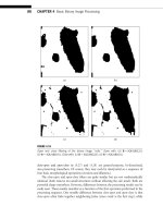
FIGURE 20.1

Three implementations of anisotropic diffusion applied to an infrared image of a tank: (a) original
noisy image; (b) results obtained using anisotropic diffusion with (20.9); (c) results obtained
using modified gradient anisotropic diffusion with (20.11) and (20.12); (d) results obtained
using morphological anisotropic diffusion with (20.11) and (20.13).
into (20.11),whereB is a structuring element of size m ϫ m, I ◦B is the morpho-
logical opening of I by B, and I •B is the morphological closing of I by B.In[13],
the open-close and close-open filters were used in an alternating manner between itera-
tions, thus reducing grayscale bias of the open-close and close-open filters. As the result
in Fig. 20.1(d) demonstrates, the morphological anisotropic diffusion method can be
used to eliminate noise and insignificant features while preserving edges. Morphological
20.3 Anisotropic Diffusion Techniques 531
anisotropic diffusion has the advantage of selecting feature scale (by specifying the
structuring element B) and selecting the gradient magnitude threshold, whereas pre-
vious anisotropic diffusions, such as (20.9) and (20.10), only allowed selection of the
gradient magnitude threshold.
You et al. introduce the following diffusion coefficient in [10]:
c(x) ϭ
⎧
⎨
⎩
1/T ϩ p(T ϩ ␧)
pϪ1
/T , ٌI(x)<T
1

|
ٌI(x)
|
ϩ p(
|

ٌI(x)
|
ϩ ␧)
pϪ1

|
ٌI(x)
|
,
|
ٌI(x)
|
Ն T ,
(20.14)
(a)
(b) (c)
FIGURE 20.2
Continued
532 CHAPTER 20 Diffusion Partial Differential Equations for Edge Detection
(d) (e)
FIGURE 20.2
(a) Corrupted “cameraman” image (Laplacian noise, SNR ϭ 13 dB) used as input for results
in Figs. 20.2(b)–(e); (b) after 8 iterations of anisotropic diffusion with (20.9), k ϭ 25; (c) after
8 iterations of anisotropic diffusion with (20.11) and (20.12), k ϭ 25; (d) after 75 iterations
of anisotropic diffusion with (20.14), T ϭ 6, e ϭ 1, p ϭ 0.5; (e) after 15 iterations of multigrid
anisotropic diffusion with (20.11) and (20.12), k ϭ 6 [35].
where the parameters are constrained by ␧ >0and0<p <1.T is a threshold on the
gradient magnitude, similar to k in (20.9). This approach has the benefits of avoiding
staircase artifacts and removing impulse noise. The main drawback is computational
expense. As seen in Fig. 20.2(d), anisotropic diffusion with this diffusion coefficient

succeeds in removing noise and retaining important features from Fig. 20.2(a), but
requires a significant number of updates.
The diffusion coefficient
c(x) ϭ
1
|
ٌI(x)
|
(20.15)
is used in mean curvature motion formulations of diffusion [14], shock filters [15], and
locally monotonic (LOMO) diffusion [16]. One may notice that this diffusion coefficient
is parameter-free.
Designing a diffusion coefficient with robust statistics, Black et al. [17] model
anisotropic diffusion as a robust estimation procedure that finds a piecewise smooth
representation of an input image. A diffusion coefficient that utilizes the Tukey’s biweight
norm is given by
c(x) ϭ
1
2

1 Ϫ

ٌI(x)
␴

2

2
(20.16)
for |ٌI (x)|Յ ␴ and is 0 otherwise. Here the parameter ␴ represents scale. Where the

standard anisotropic diffusion coefficient as in (20.9) continues to smooth over edges
20.3 Anisotropic Diffusion Techniques 533
while iterating, the robust formulation (20.16) preserves edges of a prescribed scale ␴
and effectively stops diffusion.
Here seven important versions of the diffusion coefficient were given that involve
tradeoffs between solution quality, solution expense, and convergence behavior. Other
research in the diffusion area focuses on the diffusion PDE itself. The next section
reveals significant modifications to the anisotropic diffusion PDE that affect fidelity to
the input image, edge quality, and convergence properties.
20.3.2 The Diffusion PDE
In addition to the basic anisotropic diffusion PDE given in Section 20.1.2, other diffusion
mechanisms may be employed to adaptively filter an image for edge detection. Nordstrom
[18] used an additional term to maintain fidelity to the input image, to avoid the selection
of a stopping time, and to avoid termination of the diffusion at a trivial solution, such as
a constant image. This PDE is given by
ѨI
t
(x)
Ѩt
Ϫ div
{
c(x)ٌI
t
(x)
}
ϭ I
0
(x) Ϫ I
t
(x). (20.17)

Obviously, the right-hand side I
0
(x) Ϫ I
t
(x) enforces an additional constraint that pena-
lizes deviation from the input image.
Just as Canny [19] modified the LoG edge detection technique by detecting zero-
crossings of the Laplacian only in the direction of the gradient, a similar edge-sensitive
approach can be taken with anisotropic diffusion. Here, the boundary-preserving diffu-
sion is executed only in the direction orthogonal to the gradient direction, whereas the
standard anisotropic diffusion schemes impede diffusion across the edge. If the rate of
change of intensit y is set proportional to the second partial derivative in the direction
orthogonal to the gradient (called ␶), we have
ѨI
t
(x)
Ѩt
ϭ
Ѩ
2
I
t
(x)
Ѩ␶
2
ϭ
|
ٌI
t
(x)

|
div

ٌI
t
(x)
|
ٌI
t
(x)
|

. (20.18)
This anisotropic diffusion model is called mean curvature motion, because it induces a
diffusion in which the connected components of the image level sets of the solution image
move in proportion to the boundary mean curvature. Several effective edge-preserving
diffusion methods have arisen from this framework including [20] and [21]. Alvarez
et al. [12] have used the mean curvature method in tandem with the regularized diffusion
coefficient of (20.11) and (20.12). The result is a processing method that preserves the
causality of edges through scale space. For edge-based hierarchical searches and multiscale
analyses, the edge causality property is extremely important.
The mean curvature method has also been given a graph theoretic interpretation
[22, 23]. Yezzi [23] treats the image as a graph in 
n
—a typical 2D grayscale image would
be a surface in 
3
where the image intensity is the third parameter, and each pixel is a
graph node. Hence a color image could be considered a surface in 
5

. The curvature
motion of the graphs can be used as a model for smoothing and edge detection. For
example, let a 3D graph s be defined by s(x)=s(x, y) =[x, y, I(x, y)] for the 2D image I
534 CHAPTER 20 Diffusion Partial Differential Equations for Edge Detection
with x =(x, y). To implement mean curvature motion on this graph, the PDE is given by
Ѩs(x)
Ѩt
ϭ h(x)n(x), (20.19)
where h(x) is the mean curvature,
h(x,y) ϭ
Ѩ
2
I(x, y)
Ѩx
2

1 ϩ

ѨI(x, y)
Ѩy

2

Ϫ 2

ѨI(x, y)
Ѩx

ѨI(x, y)
Ѩy



Ѩ
2
I(x, y)
ѨxѨy

ϩ
Ѩ
2
I(x, y)
Ѩy
2

1 ϩ

ѨI(x, y)
Ѩx

2

2

1 ϩ

ѨI(x, y)
Ѩy

2
ϩ


ѨI(x, y)
Ѩy

2

3/2
,
(20.20)
and n(x) is the unit normal of the surface:
n(x, y) ϭ

Ϫ
ѨI(x,y)
Ѩx
,Ϫ
ѨI(x,y)
Ѩx
,1


1 ϩ

ѨI(x,y)
Ѩy

2
ϩ

ѨI(x,y)

Ѩy

2
. (20.21)
For a discrete implementation, the partial derivatives of I (x,y) may be approximated
using simple differences. One-sided differences or central differences may be employed.
For example, a one-sided difference approximation for ѨI (x, y)/Ѩx is I(x ϩ 1,y) Ϫ
I(x,y). A central difference approximation for the same partial derivative is given by
1
2
[I(x ϩ 1,y) Ϫ I( x Ϫ 1,y)].
The standard mean curvature PDE (20.19) has the drawback of edge movement that
sacrifices edge sharpness. A remedy to this undesired movement is the use of projected
mean curvature vectors. Let z denote the unit vector in the vertical (intensity) direction
on the graph s. The projected mean curvature diffusion PDE can be formed by
Ѩs(x)
Ѩt
ϭ

h(x)n(x)

· z

z. (20.22)
The PDE for updating image intensity is then
ѨI(x)
Ѩt
ϭ
⌬I(x,y) ϩ k
2



ѨI(x,y)
Ѩx

2

Ѩ
2
I(x,y)
Ѩy
2

Ϫ 2

ѨI(x,y)
Ѩx

ѨI(x,y)
Ѩy

Ѩ
2
I(x,y)
ѨxѨy

ϩ

ѨI(x,y)
Ѩy


2

Ѩ
2
I(x,y)
Ѩx
2



1 ϩ k
2

ٌI(x,y)

2

2
,
(20.23)
where k scales the intensity variable. When k is zero, we have isotropic diffusion, and
when k becomes larger, we have a damped geometric heat equation that preserves edges
but diffuses more slowly. The projected mean curvature PDE gives edge preservation
through scale space.
Another anisotropic diffusion technique leads to LOMO signals [16]. Unlike previous
diffusion techniques that diverge or converge to trivial signals,LOMO diffusion converges
rapidly to well-defined LOMO signals of the desired degree. (A sig nal is LOMO of degree
20.3 Anisotropic Diffusion Techniques 535
d (LOMO-d) if each interval of length d is nonincreasing or nondecreasing.) Theproperty

of local monotonicity allows both slow and rapid signal transitions (ramp and step edges)
while excluding outliers due to noise. The degree of local monotonicity defines the
signal scale. In contrast to other diffusion methods, LOMO diffusion does not require
an additional regularization step to process a noisy signal and uses no thresholds or
ad hoc parameters.
On a 1D signal, the basic LOMO diffusion operation is defined by (20.6) with ⌫ϭ2
and using the diffusion coefficient (20.15), yields
[
I(x)
]
tϩ1
←

I(x) ϩ (1/2)

sign
[
ٌ
I
1
(x)
]
ϩ sign
[
ٌ
I
2
(x)
]


t
, (20.24)
where a time step of ⌬T ϭ 1/2 is used. Equation (20.24) is modified for the case where
the simple difference ٌI
1
(x) or ٌI
2
(x) is zero. Let ٌI
1
(x) ←ϪٌI
2
(x) in the case of
ٌI
1
(x) ϭ 0; ٌI
2
(x) ←ϪٌI
1
(x) when ٌI
2
(x) ϭ 0. The fixed point of (20.24) is defined
as ld(I, h
1
,h
2
),whereh
1
and h
2
are the sample spacings used to compute the simple

differences ٌI
1
(x) and ٌI
2
(x), respectively (see (20.7) and (20.8)). Let ld
d
(I) denote the
LOMO diffusion sequence that gives a LOMO-d signal from the input I. For odd values
of d =2m +1,
ld
d
(I) ϭ ld

ld

ld

ld(I, m , m),m Ϫ 1,m

,m Ϫ 1,m Ϫ 1

,1,1

. (20.25)
In (20.25), the process commences with ld(I,m,m) and continues with spacings of
decreasing widths untilld(I,1,1) is implemented. For even values of d ϭ 2m,thesequence
of operations is similar:
ld
d
(I) ϭ ld


ld

ld

ld(I, m Ϫ 1,m), m Ϫ 1, m Ϫ 1

,m Ϫ 2,m Ϫ 1

,1,1

. (20.26)
To extend this method to two dimensions, the same procedure may be followed
using (20.6) with ⌫ϭ4 [16]. Another possibility is diffusing orthogonal to the gradient
direction at each point in the image, using the 1D LOMO diffusion. Examples of 2D
LOMO diffusion and the associated edge detection results are given in Section 20.4.
20.3.3 Variational Formulation
The diffusionPDEs discussed thus far may be considered numerical methods that attempt
to minimize a cost or energy functional. Energy-based approaches to diffusion have been
effective for edge detection and image segmentation. Morel and Solimini [24] give an
excellent overview of the variational methods. Isotropic diffusion via the heat diffusion
equation leads to a minimization of the following energy:
E(I) ϭ

⍀
|
ٌI(x)
|
2
dx. (20.27)

Given an initial image I
0
, the intermediate diffusion solutions may be considered a
descent on
E(I) ϭ ␭
2

⍀
|
ٌI(x)
|
2
dx ϩ

⍀

I(x) Ϫ I
0
(x)

2
dx, (20.28)
where the regularization parameter ␭ denotes scale [24].
536 CHAPTER 20 Diffusion Partial Differential Equations for Edge Detection
Likewise, anisotropic diffusion has a variational formulation. The energy associated
with the Perona and Malik diffusion is
E(I) ϭ ␭
2

⍀

C

|
ٌI(x)
|
2

dx ϩ

⍀
[
I(x) Ϫ I
0
(x)
]
2
dx, (20.29)
where C is the integral of cЈ(x) with respect to the independent variable |ٌI(x)|
2
.Here
cЈ(x), as a function of |ٌI(x)|
2
, is equivalent to the diffusion coefficient c(x) as a function
of |ٌI(x)|,socЈ(|ٌI(x)|
2
) ϭ c(|ٌI(x)|).TheNordstrom [18] diffusion PDE (20.17)
yields steepest descent on this energy functional.
Teboul et al. have introduced a variational method that preserves edges and is useful
for edge detection. In their approach, image enhancement and edge preservation are
treated as two separate processes. The energy functional is given by

E(I,e) ϭ ␭
2

⍀

e(x)
2
|
ٌI(x)
|
2
ϩ k(e(x) Ϫ 1)
2

dx ϩ
␣
2
k

⍀
␸(
|
ٌe(x)
|
)dx ϩ

⍀
[
I(x) Ϫ I
0

(x)
]
2
dx,
(20.30)
where the real-valued variable e(x) is the edge strength at position x, and e(x) ∈[0,1].In
(20.30), the diffusion coefficient is defined by c(|ٌI(x)|) ϭ ␸Ј(|ٌI(x )|)/2( |ٌI (x)|).An
additional regularization parameter ␣ is needed, and k is essentially an edge threshold
parameter.
The energy functional in (20.30) leads to a system of two coupled PDEs:
I
0
(x) Ϫ I
t
(x) Ϫ ␭
2
div

e(x)

ٌI
t
(x)

ٌI
t
(x)

ϭ 0 (20.31)
and

e(x)

|
ٌI(x)
|
2
k
ϩ 1

Ϫ 1ϩ
␣
2
k
2
div

c(
|
ٌe(x)
|
)ٌe(x)

ϭ 0. (20.32)
The coupled PDEs have the advantage of edge preservation within the adaptive smoot-
hing process. An edge map can be directly extracted from the final state of e.
This edge-preserving variational method is related to the segmentation approach of
Mumford and Shah [25]. The energy functional to be minimized is
E(I) ϭ ␭
2


⍀\⌿
|
ٌI(x)
|
2
dx ϩ

⍀\⌿
[
I(x) Ϫ I
0
(x)
]
2
dx ϩ ␮␭
2

⌿
d␺, (20.33)
where

⌿
d␺ is the integrated length of the edges (Hausdorff measure), ⍀\⌿ is the set
of image locations that exclude the edge positions, and ␮ is an additional weight parame-
ter. The a dditional edge-length term reflects the goal of computing a minimal-length edge
map for a given scale ␭. The Mumford-Shah functional has spurred several variational
image segmentation schemes, including PDE-based solutions [24].
In edge detection, thin, contiguous edges are typically desired. With diffusion-based
edge detectors,the edges may be“thick”or“broken”when agradient magnitude threshold
20.3 Anisotropic Diffusion Techniques 537

is applied after diffusion. The variational formulation allows the addition of additional
constraints that promote edge thinning and connectivity. Black et al. used two additional
terms, a hysteresis term for improved connectivity and a nonmaximum suppression term
for thinning [17]. A similar approach was taken in [26]. The additional terms allow the
effective extraction of spatially coherent outliers. This idea is also found in the design of
line processes for regularization [27].
20.3.4 Multiresolution Diffusion
One drawback of diffusion-based edge detection is the computational expense. Typically,
a large number (anywhere from 20 to 200) of iterative steps are needed to provide a
high-quality edge map. One solution to this dilemma is the use of multiresolution
schemes. Two such approaches have been investigated for edge detection: the anisotropic
diffusion pyramid and multigrid anisotropic diffusion.
In the case of isotropic diffusion, the Gaussian pyramid has been used for edge detec-
tion and image segmentation [28, 29]. The basic idea is that the scale generating operator
(a Gaussian filter, for example) can be used as an antialiasing filter before sampling. Then,
a set of image representations of increasing scale and decreasing resolution (in terms of
the number of pixels) can be generated. This image pyramid can be used for hierarchical
searches and coarse-to-fine edge detection.
The anisotropic diffusion pyramids [30, 31] are born from the same fundamen-
tal motivation as their isotropic, linear counterparts. However, with a nonlinear scale-
generating operator, the presampling operation is constrained morphologically, not by
the tr aditional sampling theorem. In the nonlinear case, the scale-generating operator
should remove image features not supported in the subsampled domain. Therefore,
morphological methods [32, 33] for creating image pyramids have also been used in
conjunction with the morphological sampling theorem [34].
The anisotropic diffusion pyramids are, in a way, ad hoc multigrid schemes. A multi-
grid scheme can be useful for diffusion-based edge detectors in two ways. First, like
the anisotropic diffusion pyramids, the number of diffusion updates may be decreased.
Second, the multigrid approach can be used to eliminate low-frequency error. The
anisotropic diffusion PDEs are stiff—they rapidly reduce hig h-frequency error (noise,

small details), but slowly reduce background variations and often create artifacts such as
blotches (false regions) or staircases (false step edges). See Fig. 20.3 for an example of a
staircasing artifact.
(a)
(b)
(c)
FIGURE 20.3
(a) Sigmoidal ramp edge; (b) after anisotropic diffusion with (9) (k ϭ 10); (c) after multigrid
anisotropic diffusion with (9) (k ϭ 10) [35].
538 CHAPTER 20 Diffusion Partial Differential Equations for Edge Detection
To implement a multigrid anisotropic diffusion operation [35], define J as an estimate
of the image I. A system of equations is defined by A(I) ϭ 0where
[
A(I)
]
(x) ϭ (⌬T )
⌫

dϭ1
c
d
(x)ٌ
I
d
(x), (20.34)
which is relaxed by the discrete anisotropic diffusion PDE (20.6). For this system of
equations, the (unknown) algebraic error is E ϭ I Ϫ J and the residual is R ϭϪA(J) for
image estimate J. The residual equation A(E) ϭ R can be relaxed (diffused) in the same
manner as (20.34) using (20.6) to form an estimate of the error.
The first step is performing ␯ diffusion steps on the original input image (level

L = 0). Then, the residual equation at the coarser grid L +1is
A(E
Lϩ1
) ϭϪA

(
J
L
)
↓S

, (20.35)
where ↓S represents downsampling by a factor of S. Now, the residual equation (20.33)
can be relaxed using the discrete diffusion PDE (20.6) with an initial error estimate of
E
Lϩ1
ϭ 0. The new error estimate E
Lϩ1
after relaxation can then be transferred to the
finer grid to correct the initial image estimate J in a simple two-gr i d scheme. Alternatively,
the process of transferring the residual to successively coarser grids can be continued until
a grid is reached in which a closed form solution is possible. Then, the error estimates
are propagated back to the original grid.
Additional steps may be taken to account for the nonlinearity of the anisotropic dif-
fusion PDE, such as implementing a full approximation scheme (FAS) multigrid system,
or by using a global linearization step in combination with a Newton method to solve
for the error iteratively [9, 19].
The results of applying multigrid anisotropic diffusion are show n in Fig. 20.2(e).In
just 15 updates, the multigrid anisotropic diffusion method was able to remove the noise
from Fig. 20.2(b) while preserving the significant objects and avoiding the introduction

of blotching artifacts.
20.3.5 Multispectral Anisotropic Diffusion
Color edge detection and boundary detection for multispectral imagery are important
tasks in general image/video processing, remote sensing, and biomedical image process-
ing. Applying anisotropic diffusion to each channel or spectral band separately is one
possible way of processing multichannel or multispectral image data. However, this sing le
band approach forfeits the richness of the multispectral data and provides individual edge
maps that do not possess corresponding edges.
Two solutions have emerged for diffusing multispectral imagery. The first, called
vector distance dissimilarity,utilizes a functionof the gradients from each bandto compute
an overall diffusion coefficient. For example, to compute the diffusion coefficient in the
“western” direction on an RGB color image, the following function could be applied:
ٌI
1
(x) ϭ


R(x Ϫ h
1
,y)ϪR(x, y)

2
ϩ

G(x Ϫ h
1
,y) Ϫ G(x,y)

2
ϩ


B(x Ϫ h
1
,y) Ϫ B(x, y)

2
,
(20.36)
20.3 Anisotropic Diffusion Techniques 539
where R(x) isthe red band intensity at x,G(x) isthe green band,and B(x) isthe blueband.
Using the vector distance dissimilarity method, the standard diffusion coefficients such as
(20.9) can be employed. This technique was used in [38] for shape-based processing and
in [39] for processing remotely sensed imagery. An example of multispectral anisotropic
diffusion is shown in Fig. 20.4. Using the noisy multispectral image in Fig. 20.4(a) as
input, the vector distance dissimilarity method produces the smoothed result shown in
Fig. 20.4(b), which has an associated image of gradient magnitude shown in Fig. 20.4(c).
As can be witnessed in Fig. 20.4(c), an edge detector based on vector distance dissimilarity
is sensitive to noise and does not identify the impor tant image boundaries.
The second method uses mean curvature motion and a multispectral gradient for-
mula to achieve anisotropic, edge-preserving diffusion. The idea behind mean curvature
motion, as discussed above, is to diffuse in the direction opposite to the gradient such
that the image level set objects move with a rate in proportion to their mean curvature.
With a grayscale image, the gradient is always perpendicular to the level set objects of the
image. In the multispectral case, this quality does not hold. A well-motivated diffusion is
defined by Sapiro and Ringach [40], using DiZenzo’s multispectral gradient formula [41].
In Fig. 20.4(d), results for multispectral anisotropic diffusion are shown for the mean
curvature approach of [40] used in combination with the modified gradient approach of
[11]. The edge map in Fig. 20.4(e) shows improved resilience to impulse noise over the
vector distance dissimilarity approach.
20.3.6 Speckle Reducing Anisotropic Diffusion

The anisotropic diffusion PDE introduced in (20.5) assumes that the image is corrupted
by additive noise. Speckle reducing anisotropic diffusion (SRAD) is a PDE technique for
image enhancement in which signal-dependent multiplicative noise is present, as with
radar and ultrasonic imaging. Whereas traditional anisotropic diffusion can be viewed
as the edge-sensitive version of classical linear filters (e.g., the Gaussian filter), SRAD
can be viewed as the edge-sensitive 3 version of classical speckle reducing filters that
emerged from the radar community (e.g., the Lee filter). SRAD smoothes the imagery
and enhances edges by inhibiting diffusion across edges and allowing isotropic diffusion
within homogeneous regions. For images containing signal-dependent, spatially corre-
lated multiplicative noise, SRAD excels over the adaptive filtering techniques designed
with additive noise models in mind.
The SRAD technique employs an adaptive speckle filter that uses a local statistic for
the coefficient of variation, defined as the ratio of standard deviation to mean, to measure
the strength of edges in speckle imagery. A discrete form of this operator in 2D is [42]
q(x) ϭ








(1/2)
|
ٌI(x)
|
2
Ϫ (1/16)(ٌ
2

I(x))
2




I(x) ϩ (1

4)ٌ
2
I(x)

2
, (20.37)
where ٌ
2
I(x) is the Laplacian of image at position x, and ٌI(x) is the gradient of image
at position x.
540 CHAPTER 20 Diffusion Partial Differential Equations for Edge Detection
(a) (b)
(c) (d)
(e)
FIGURE 20.4
(a) SPOT multispectral image of the Seattle area, with additive Gaussian-distributed noise,
␴ ϭ 10; (b) Vector distance dissimilarity diffusion result, using diffusion coefficient in (20.9);
(c) Edges (gradient magnitude) from result in (b); (d) Mean curvature motion (20.18) result
using diffusion coefficient from (20.11) and (20.12); (e) Edges (gradient magnitude) from
result in (d).
20.3 Anisotropic Diffusion Techniques 541
(a) (b) (c)

FIGURE 20.5
(a) An ultrasound image of a prostate phantom with implanted radioactive seeds; (b) correspond-
ing SRAD-diffused image; (c) corresponding ICOV edge strength image [43].
The operator q( x) is called the instantaneous coefficient of variation (ICOV). The
ICOV uses the absolute value of the difference of a normalized gradient magnitude and
a normalized Laplacian operator to measure the strength of edges in speckled imagery.
The normalizing function I(x) ϩ (1
/
4)ٌ
2
I(x) gives a smoothed version of the image at
position x. This term compensates for the edge measurement localization error. The
ICOV allows for balanced and well-localized edge strength measurements in bright
regions as well as in dark regions. It has been shown that the ICOV operator optimizes
the edge detection in speckle imagery in terms of low false edge detection probability
and high edge localization accuracy [43]. Figure 20.5 shows an example of an ultrasound
image (Fig. 20.5(a)) that has been processed by SRAD (Fig. 20.5(b)) and where edges are
displayed using the ICOV values (Fig. 20.5(c)).
Given an intensity image I having no zero-valued intensities over the image domain,
the output image is evolved according to the following PDE:
ѨI
t
(x)/Ѩt ϭ div

c

q(x)

ٌI
t

(x)

, (20.38)
where ٌ is the gradient operator, div is the divergence operator, and || denotes the
magnitude. The diffusion coefficient c(q(x)) is given by
c

q(x)

ϭ

1 ϩ

q
2
(x) Ϫ ˜q
2
(x)

˜q
2
(x)(1 ϩ ˜q
2
(x))

Ϫ1
, (20.39)
where q(x) is the ICOV as determined by (20.37), and ˜q(x) is the current speckle noise
level. Example input and output images from an ultrasound image of the human heart
are shown in Fig. 20.6.

The diffusion coefficient c(q(x)) is proportional to the likelihood that a point x is in a
homogeneous speckle region at the update time. From (20.39),it is seen that the diffusion
coefficient exhibits nearly zero values at edges with high contrast (i.e., q(x)>>˜q(x)),
while in homogeneous speckle regions, the coefficient approaches unity. Hence, it is the
542 CHAPTER 20 Diffusion Partial Differential Equations for Edge Detection
FIGURE 20.6
(Left) Speckled ultrasound image of left ventricle in a human heart prior to SRAD; (right) same
image after SRAD enhancement.
diffusion coefficient that allows isotropic diffusion in homogeneous speckle regions and
prohibits diffusion across the edges.
The implementation issues connected with anisotropic diffusion include specification
of the diffusion coefficient and diffusion PDE, as discussed above. The anisot ropic diffu-
sion method can be expedited through multiresolution implementations. Furthermore,
anisotropic diffusion can be extended to multispectral imagery and to ultrasound/radar
imagery. In the following section, we discuss the specific application of anisotropic
diffusion to edge detection.
20.4 APPLICATION OF ANISOTROPIC DIFFUSION TO EDGE
DETECTION
20.4.1 Edge Detection by Thresholding
Once anisotropic diffusionhas beenapplied to an imageI,aprocedureneedstobedefined
to extract the image edges e. The most typical procedure is to simply define a gradient
magnitude threshold, T , that defines the location of an edge. For example, e(x) ϭ 1if
|ٌI(x)| > T and e(x) ϭ 0 otherwise. Of course, the question becomes one of selecting a
proper value for T. With typical diffusion coefficients such as (20.9) and (20.10), T ϭ k
is often asserted. Another approach is to use the diffusion coefficient itself as the measure
of edge strength: e(x) ϭ 1ifc(x)<T and e(x) ϭ 0 otherwise.
T ϭ ␴
e
of the image, as defined in [44]: ␴
e

ϭ 1.4826med{|ٌI(x) Ϫ med(|ٌI(x)|)|}
where the med operator is the median performed over the entire image domain ⍀.
The constant used (1.4826) is derived from the mean absolute deviation of the normal
distribution with unit variance [17].
20.4 Application of Anisotropic Diffusion to Edge Detection 543
20.4.2 Edge Detection from Image Features
Aside from thresholding the gradient magnitude of a diffusion result, a feature detection
approach may be used. As with Marr’s classical LoG detector, the inflection points of a
diffused image may be located by finding the zero-crossing in a Laplacian-convolved
result. However, if the anisotropic diffusion operation produces piecewise constant
images as in [10, 17], the g radient magnitude is sufficient to define thin, contiguous
edges.
With LOMO diffusion, other features that appear in the diffused image may be used
for edge detection. An advantage of LOMO diffusion is that no threshold is required for
edge detection. LOMO diffusion segments each row and column of the image into ramp
segments and constant segments. Within this fr amework, we can define concave-down,
concave-up, and ramp center edge detection processes. Consider an image row or column.
With a concave-down edge detection,the ascending (increasing intensity) segments mark
the beginning of an object and the descending (decreasing intensity) segments terminate
the object. With a concave-up edge detection, negative-going objects (in intensity) are
detected. The ramp center edge detection sets the boundary points at the centers of the
ramp edges, as the name implies. When no bias toward bright or dark objects is present,
a ramp center edge detection can be utilized.
Figure 20.7 provides two examples of feature-based edge detection using LOMO
diffusion. The images in Fig. 20.7(b) and (e) are the results of applying 2D LOMO
diffusion to Fig. 20.7(a) and (d), respectively. The concave-up edge detection given
in Fig. 20.7(c) reveals the boundaries of the blood cells. In Fig. 20.7(f), a ramp cen-
ter edge detection is used to find the boundaries between the aluminum grains of
Fig. 20.7(d).
20.4.3 Quantitative Evaluation of Edge Detection by Anisotropic

Diffusion
When choosing a suitable anisotropic diffusion process for edge detection, one may
evaluate the results qualitatively or use an objective measure. Three such quantitative
assessment tools include the percentage of edges correctly identified as edges, the percent-
age of false edges, and Pratt’s edge quality metric. Given ground truth edge information,
usually with synthetic data, one may measure the correlation between the ideal edge map
and the computed edge map. This correlation leads to a classification of “correct” edges
(where the computed edge map and ideal version match) and “false” edges. Another
method utilizes Pratt’s edge quality measurement [45]:
F ϭ
I
A

iϭ1
1
1 ϩ ␣

d(i)
2

max
{
I
A
,I
I
}
, (20.40)
where I
A

is the number of edge pixels detected in the diffused image result, I
I
is the
number of edge pixels existing in the original, noise free imagery, d(i) is the Euclidean