The Essential Guide to Image Processing- P19 ppt

20.6 Conclusions 549
(a) (b)
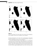
FIGURE 20.11
(a) In tracking a white blood cell, the GVF vector diffusion fails to attract the active contour;
(b) successful detection is yielded by MGVF.
Thus (20.48) provides an external force that can guide an active contour to a moving
object boundary. The capture range of GVF is increased using the motion gradient
vector flow (MGVF) vector diffusion [51]. With MGVF, a tracking algorithm can simply
use the final position of the active contour from a prev ious video frame as the initial
contour in the subsequent frame. For an example of tracking using MGVF, see Fig. 20.11.
20.6 CONCLUSIONS
Anisotropic diffusion is an effective precursor to edge detection. The main benefit of
anisotropic diffusion over isotropic diffusion and linear filtering is edge preservation.
By properly specifying the diffusion PDE and the diffusion coefficient, an image can
be scaled, denoised, and simplified for boundary detection. For edge detection, the
most critical design step is specification of the diffusion coefficient. The variants of
the diffusion coefficient involve tr adeoffs between sensitivity to noise, the ability to spec-
ify scale, convergence issues, and computational cost. The diverse implementations of
the anisotropic diffusion PDE result in improved fidelity to the original image, mean
curvature motion, and convergence to LOMO signals. As the diffusion PDE may be
considered a descent on an energy surface, the diffusion operation can be viewed in a
variational framework. Recent variational solutions produce optimized edge maps and
image segmentations in which certain edge-based features,such as edge length, curvature,
thickness, and connectivity, can be optimized.
The computational cost of anisotropic diffusion may be reduced by using multireso-
lution solutions, including the anisotropic diffusion pyramid and multigrid anisotropic
diffusion. Application of edge detection to multispectral imagery and to radar/ultrasound
imagery is possible through techniques presented in the literature. In general, the edge
detection step after anisotropic diffusion of the image is straightforward. Edges may be
detected using a simple gradient magnitude threshold, using robust statistics, or using a
550 CHAPTER 20 Diffusion Partial Differential Equations for Edge Detection

feature extraction technique. Active contours, used in conjunction with vector diffusion,
can be employed to extract meaningful object boundaries.
REFERENCES
[1] D. G. Lowe. Perceptual Organization and Visual Recognition. Kluwer Academic, New York, 1985.
[2] V. Caselles, J M. More l, G. Sapiro, and A. Tannenbaum. Introduction to the special issue on partial
differential equations and geometry-driven diffusion in image processing and analysis. IEEE Trans.
Image Process., 7:269–273, 1998.
[3] A. P. Witkin. Scale-space filtering. In Proc. Int. Joint Conf. Art. Intell., 1019–1021, 1983.
[4] J. J. Koenderink. The structure of images. Biol. Cybern., 50:363–370, 1984.
[5] D. Marr and E. Hildreth. Theory of edge detection. Proc. R. Soc. Lond. B, Biol. Sci., 207:187–217,
1980.
[6] P. Perona and J. Malik. Scale-space and edge detection using anisotropic diffusion. IEEE Trans.
Pattern Anal. Mach. Intell., PAMI-12:629–639, 1990.
[7] S. Teboul, L. Blanc-Feraud, G. Aubert, and M. Barlaud. Variational approach for edge-preserving
regularization using coupled PDE’s. IEEE Trans. Image Process., 7:387–397, 1998.
[8] R. T. Whitaker and S. M. Pizer. A multi-scale approach to nonuniform diffusion. Comput. Vis.
Graph. Image Process.—Image Underst., 57:99–110, 1993.
[9] Y L. You, M. Kaveh, W. Xu, and A. Tannenbaum. Analysis and design of anisotropic diffusion
for image processing. In Proc. IEEE Int. Conf. Image Process., Austin, Texas, November 13–16,
1994.
[10] Y L. You, W. Xu, A. Tannenbaum, and M. Kaveh. Behavioral analysis of anisotropic diffusion in
image processing. IEEE Trans. Image Process., 5:1539–1553, 1996.
[11] F. Catte, P L. Lions, J M. More l, and T. Coll. Image selective smoothing and edge detection by
nonlinear diffusion. SIAM J. Numer. Anal., 29:182–193, 1992.
[12] L. Alvarez, P L. Lions, and J M. Morel. Image selective smoothing and edge detection by nonlinear
diffusion II. SIAM J. Numer. Anal., 29:845–866, 1992.
[13] C. A. Segall and S. T. Acton. Morphological anisotropic diffusion. In Proc. IEEE Int. Conf. Image
Process., Santa Barbara, CA, October 26–29, 1997.
[14] L I. Rudin, S. Osher, and E. Fatemi. Nonlinear total variation noise removal algorithm. Physica D,
60:1217–1229, 1992.

[15] S. Osher and L I. Rudin. Feature-oriented image enhancement using shock filters. SIAM J. Numer.
Anal., 27:919–940, 1990.
[16] S. T. Acton. Locally monotonic diffusion. IEEE Trans. Signal. Process., 48:1379–1389, 2000.
[17] M. J. Black, G. Sapiro, D. H. Marimont, and D. He eger. Robust anisotropic diffusion. IEEE Trans.
Image. Process., 7:421–432, 1998.
[18] K. N. Nordstrom. Biased anisotropic diffusion—a unified approach to edge detection. Tech. Report,
Dept. of Electrical Engineering and Computer Sciences, University of California at Berkeley,
Berkeley, CA, 1989.
[19] J. Canny. A computational approach to edge detection. IEEE Trans. Pattern Anal. Mach. Intell.,
PAMI-8:679–714, 1986.
References 551
[20] A. El-Fallah and G. Ford. The evolution of mean curvature in image filtering. In Proc. IEEE Int.
Conf. Image Process., Austin, Texas, November 1994.
[21] S. Osher and J. Sethian. Fronts propagating with curvature dependent speed: algorithms based on
the Hamilton-Jacobi formulation. J. Comp. Phys., 79:12–49, 1988.
[22] N. Sochen, R. Kimmel, and R. Malladi. A general framework for low level vision. IEEE Trans. Image
Process., 7:310–318, 1998.
[23] A. Yezzi, Jr. Modified curvature motion for image smoothing and enhancement. IEEE Trans. Image
Process., 7:345–352, 1998.
[24] J L. Morel and S. Solimini. Variational Methods in Image Segmentation. Birkhauser, Boston, MA,
1995.
[25] D. Mumford and J. Shah. Boundary detection byminimizingfunctionals.In IEEE Int. Conf. Comput.
Vis. Pattern Recognit., San Francisco, 1985.
[26] S. T. Acton and A. C. Bovik. Anisotropic edge detection using mean field annealing. In Proc. IEEE
Int. Conf. Acoust., Speech and Signal Process. (ICASSP-92), San Francisco, March 23–26, 1992.
[27] D. Geman and G. Reynolds. Constrained restoration and the re covery of discontinuities. IEEE
Trans. Pattern Anal. Mach. Intell., 14:376–383, 1992.
[28] P. J. Burt, T. Hong, and A. Rosenfeld. Segmentation and estimation of region properties through
cooperative hierarchical computation. IEEE Trans. Syst. Man Cybern., 11(12):1981.
[29] P. J. Burt. Smart s ensing within a pyramid vision machine. Proc. IEEE, 76(8):1006–1015, 1988.

[30] S. T. Acton. A pyramidal edge detector based on anisotropic diffusion. In Proc. of the IEEE Int. Conf.
Acoust., Speech and Signal Process. (ICASSP-96), Atlanta, May 7–10, 1996.
[31] S. T. Acton, A. C. Bovik, and M. M. Crawford. Anisotropic diffusion pyramids for image
segmentation. In Proc. IEEE Int. Conf. Image Process., Austin, Texas, November 1994.
[32] A. Morales, R. Acharya, and S. Ko. Morphological pyramids with alternating sequential filters.
IEEE Trans. Image Process., 4(7):965–977, 1996.
[33] C. A. Segall, S. T. Acton, and A. K. Katsaggelos. Sampling conditions for anisotropic diffusion. In
Proc. SPIE Symp. Vis. Commun. Image Process., San Jose, January 23–29, 1999.
[34] R. M. Haralick, X. Zhuang, C. Lin, and J. S. J. Lee. The digital morphological sampling theorem.
IEEE Trans. Acoust., 3720(12):2067–2090, 1989.
[35] S. T. Acton. Multigrid anisotropic diffusion. IEEE Trans. Image. Process., 7:280–291, 1998.
[36] J. H. Bramble. Multigrid Methods. John Wiley, New York, 1993.
[37] W. Hackbush and U. Trottenberg, editors. Multigrid Methods. Springer-Verlag, New York, 1982.
[38] R. T. Whitaker and G. Gerig. Vector-valued diffusion. In B. ter Haar Romeny, editor, Geometry-
Driven Diffusion in Computer Vision, 93–134. Kluwer, 1994.
[39] S. T. Acton and J. Landis. Multispectr al anisotropic diffusion. Int. J. Remote Sens., 18:2877–2886,
1997.
[40] G. Sapiro and D. L. Ringach. Anisotropic diffusion of multivalued images with applications to color
filtering. IEEE Trans. Image Process., 5:1582–1586, 1996.
[41] S. DiZenzo. A note on the gradient of a multi-image. Comput. Vis. Graph. Image Process., 33:
116–125, 1986.
[42] Y. Yu and S. T. Acton. Speckle reducing anisotropic diffusion. IEEE Trans. Image Process., 11:
1260–1270, 2002.
552 CHAPTER 20 Diffusion Partial Differential Equations for Edge Detection
[43] Y. Yu and S. T. Acton. Edge detection in ultrasound imagery using the instantaneous coefficient of
variation. IEEE Trans. Image Process., 13(12):1640–1655, 2004.
[44] P. J. Rousseeuw and A. M. Leroy. Robust Regression and Outlier Detection. Wiley, New York, 1987.
[45] W. K. Pratt. D i gital Image Processing. Wiley, New York, 495–501, 1978.
[46] M. Kass, A. Witkin, and D. Terzopoulos. Snakes: active contour models. Int. J. Comput. Vis.,
1(4):321–331, 1987.

[47] R. Courant and D. Hilbert. Methods of Mathematical Physics, Vol. 1. Interscience Publishers Inc.,
New York, 1953.
[48] J. L. Troutman. Variational Calculus with Elementary Convexity. Springer-Verlag, New York, 1983.
[49] C. Xu and J. L. Prince. Snakes, shapes, and gradient vector flow. IEEE Trans. Image Process.,
7: 359–369, 1998.
[50] C. Xu and J. L. Prince. Generalized gradient vector flow external force for active contours. Signal
Processing, 71:131–139, 1998.
[51] N. Ray and S. T. Acton. Tracking rolling leukocytes with motion gradient vector flow. In Proc.
37th Asilomar Conf. on Signals, Systems and Computers, Pacific Grove, California, November 9–12,
2003.
CHAPTER
21
Image Quality Assessment
Kalpana Seshadrinathan
1
, Thrasyvoulos N. Pappas
2
,
Robert J. Safranek
3
, Junqing Chen
4
, Zhou Wang
5
,
Hamid R. Sheikh
6
, and Alan C. Bovik
7
1

The University of Texas at Austin;
2
Northwestern University;
3
Benevue, Inc.;
4
Northwestern University;
5
University of Waterloo;
6
Texas Instruments, Inc.;
7
The University of Texas at Austin
21.1 INTRODUCTION
Recent advances indigital imaging technolog y, computational speed,storage capacity,and
networking have resulted in the proliferation of digital images, both still and video. As the
digital images are captured, stored, transmitted, and displayed in different devices, there
is a need to maintain image quality. The end users of these images, in an overwhelmingly
large number of applications, are human observers. In this chapter, we examine objective
criteria for the evaluation of image quality as perceived by an average human observer.
Even though we use the term image quality, we are primarily interested in image fidelity,
i.e., how close an image is to a given original or reference image. This paradigm of image
quality assessment (QA) is also known as full reference image QA. The development of
objective metrics for evaluating image quality without a reference image is quite different
and is outside the scope of this chapter.
Image QA plays a fundamental role in the design and evaluation of imaging and
image processing systems. As an example, QA algorithms can be used to systematically
evaluate the performance of different image compression algorithms that attempt to
minimize the number of bits required to store an image, while maintaining sufficiently
high image qualit y. Similarly, QA algorithms can be used to evaluate image acquisition

and display systems. Communication networks have developed tremendously over the
past decade, and images and video are frequently transported over optic fiber, p acket
switched networks like the Internet, wireless systems, etc. Bandwidth efficiency of appli-
cations such as video conferencing and Video on Demand can be improved using QA
systems to evaluate the effects of channel errors on the transported images and video.
Further, QA algorithms can be used in “perceptually optimal” design of various compo-
nents of an image communication system. Finally, QA and the psychophysics of human
vision are closely related disciplines. Research on image and video QA may lend deep
553
554 CHAPTER 21 Image Quality Assessment
insights into the functioning of the human visual system (HVS), which would be of
great scientific value.
Subjective evaluations are accepted to be the most effective and reliable, albeit quite
cumbersome and expensive, way to assess image quality. A significant effort has been
dedicated for the development of subjective tests for image quality [56, 57]. There has
also been standards activity on subjective evaluation of image quality [58]. The study of
the topic of subjective evaluation of image quality is beyond the scope of this chapter.
The goal of an objective perceptual metric for image quality is to determine the
differences between two images that are visible to the HVS. Usually one of the images is
the reference which is considered to be“orig inal,”“perfect,”or “uncorrupted.”The second
image has been modified or distorted in some sense. The output of the QA algorithm is
often a number that represents the probability that a human eye can detect a difference in
the two images or a number that quantifies the perceptual dissimilarity between the two
images. Alternatively, the output of an image quality metric could be a map of detection
probabilities or perceptual dissimilarity values.
Perhaps the earliest image quality metrics were the mean squared error (MSE) and
peak signal-to-noise ratio (PSNR) between the reference and distorted images. These
metrics are still widely used for performance evaluation, despite their well-known lim-
itations, due to their simplicity. Let f (n) and g (n) represent the value (intensity) of an
image pixel at location n. Usually the image pixels are arranged in a Cartesian grid and

n ϭ (n
1
,n
2
). The MSE between f (n) and g(n) is defined as
MSE

f (n),g(n)

ϭ
1
N

n

f (n) Ϫ g (n)

2
, (21.1)
where N is the total number of pixel locations in f (n) or g (n). The PSNR between these
image patches is defined as
PSNR

f (n),g(n)

ϭ 10 log
10
E
2
MSE


f (n),g(n)

, (21.2)
where E is the maximum value that a pixel can take. For example, for 8-bit grayscale
images, E ϭ 255.
In Fig. 21.1, we show two distorted images generated from the same or iginal image.
The first distorted image (Fig. 21.1(b)) was obtained by adding a constant number to
all signal samples. The second distorted image (Fig. 21.1(c)) was generated using the
same method except that the signs of the constant were randomly chosen to be positive
or negative. It can be easily shown that the MSE/PSNR between the original image and
both of the distorted images are exactly the same. However, the visual quality of the two
distorted images is drastically different. Another example is shown in Fig. 21.2,where
Fig. 21.2(b) was generated by adding independent white Gaussian noise to the original
texture image in Fig. 21.2(a).InFig. 21.2(c), the signal sample values remained the same
as in Fig. 21.2(a), but the spatial ordering of the samples has been changed (through
a sorting procedure). Figure 21.2(d) was obtained from Fig. 21.2(b), by following the
same reordering procedure used to create Fig. 21.2(c). Again, the MSE/PSNR between
21.2 Human Vision Modeling Based Metrics 555
(a)
(b) (c)
1
1
FIGURE 21.1
Failure of the Minkowski metric for image quality prediction. (a) original image; (b) distorted
image by adding a positive constant; (c) distorted image by adding the same constant, but with
random sign. Images (b) and (c) have the same Minkowski metric with respect to image (a), but
drastically different visual quality.
Figs. 21.2(a) and 21.2(b) and Figs. 21.2(c) and 21.2(d) is exactly the same. However,
Fig. 21.2(d) appears to be significantly noisier than Fig. 21.2(b).

The above examples clearly illustrate the failure of PSNR as an adequate measure
of visual quality. In this chapter, we will discuss three classes of image QA algorithms
that correlate with visual perception significantly better—human vision based metrics,
Structural SIMilarity (SSIM) metrics, and information theoretic metrics. Each of these
techniques approaches the image QA problem from a different perspective and using
different first principles. As we proceed in this chapter, in addition to discussing these
QA techniques, we will also attempt to shed light on the similarities, dissimilarities, and
interplay between these seemingly diverse techniques.
21.2 HUMAN VISION MODELING BASED METRICS
Human vision modeling based metrics utilize mathematical models of certain stages of
processing that occur in the visual systems of humans to construct a quality metric.
Most HVS-based methods take an engineering approach to solving the QA problem by
556 CHAPTER 21 Image Quality Assessment
Noise
(a)
Reordering
pixels
(b) (d)
(c)
1
FIGURE 21.2
Failure of the Minkowski metric for image quality prediction. (a) original texture image; (b) dis-
torted image by adding independent white Gaussian noise; (c) reordering of the pixels in image
(a) (by sorting pixel intensity values); (d) reordering of the pixels in image (b), by following the
same reordering used to create image (c). The Minkowski metrics between images (a) and (b)
and images (c) and (d) are the same, but image (d) appears much noisier than image (b).
measuring the threshold of visibility of signals and noise in the signals. These thresholds
are then utilized to normalize the error between the reference and distorted images to
obtain a perceptually meaningful error metric. To measure visibility thresholds, differ-
ent aspects of visual processing need to be taken into consideration such as response

to average brightness, contrast, spatial frequencies, orientations, etc. Other HVS-based
methods attempt to directly model the different stages of processing that occur in the
HVS that results in the observed visibility thresholds. In Section 21.2.1, we will discuss the
individual building blocks that comprise a HVS-based QA system. The function of these
blocks is to model concepts from the psychophysics of human perception that apply to
image quality met rics. In Section 21.2.2, we will discuss the details of several well-known
HVS-based QA systems. Each of these QA systems is comprised of some or all of the
building blocks discussed in Section 21.2.1, but uses different mathematical models for
each block.
21.2.1 Building Blocks
21.2.1.1 Preprocessing
Most QA algorithms include a preprocessing stage that typically comprises of calibra-
tion and registration. The array of numbers that represents an image is often mapped to
21.2 Human Vision Modeling Based Metrics 557
units of visual frequencies or cycles per degree of visual angle, and the calibration stage
receives input parameters such as viewing distance and physical pixel spacings (screen
resolution) to perform this mapping. Other calibration parameters may include fixa-
tion depth and eccentricity of the images in the observer’s visual field [37, 38]. Display
calibration or an accurate model of the display device is an essential part of any image
quality metric [55], as the HVS can only see what the display can reproduce. Many qual-
ity metrics require that the input image values be converted to physical luminances
1
before they enter the HVS model. In some cases, when the perceptual model is obtained
empirically, the effects of the display are incorporated in the model [40]. The obvious
disadvantage of this approach is that when the display changes, a new set of model
parameters must be obtained [43]. The study of display models is beyond the scope of
this chapter.
Registration, i.e., establishing point-by-point correspondence between two images, is
also necessary in most image QA systems. Often times, the performance of a QA model
can be extremely sensitive to registration errors since many QA systems operate pixel by

pixel (e.g., PSNR) or on local neighborhoods of pixels. Errors in registration would result
in a shift in the pixel or coefficient values being compared and degrade the performance
of the system.
21.2.1.2 Frequency Analysis
The f requency analysis stage decomposes the reference and test images into different
channels (usually called subbands) with different spatial frequencies and orientations
using a set of linear filters. In many QA models, this stage is intended to mimic simi-
lar processing that occurs in the HVS: neurons in the visual cortex respond selectively
to stimuli with particular spatial frequencies and orientations. Other QA models that
target specific image coders utilize the same decomposition as the compression sys-
tem and model the thresholds of visibility for each of the channels. Some examples of
such decompositions are shown in Fig. 21.3. The range of each axis is from Ϫu
s
/2to
u
s
/2 cycles per degree, where u
s
is the sampling frequency. Figures 21.3(a)–(c) show
transforms that are polar separable and belong to the former category of decomposi-
tions (mimicking processing in the visual cortex). Figures 21.3(d)–(f) are used in QA
models in the latter category and depict transforms that are often used in compression
systems.
In the remainder of this chapter, we will use f (n) to denote the value (intensity,
grayscale, etc.) of an image pixel at location n. Usually the image pixels are arranged
in a Cartesian grid and n ϭ (n
1
,n
2
). The value of the kth image subband at location

n will be denoted by b(k,n). T he subband indexing k ϭ (k
1
,k
2
) could be in Cartesian
or polar or even scalar coordinates. The same notation will be used to denote the kth
coefficient of the nth discrete cosine transform (DCT) block (both Cartesian coordinate
systems). This notation underscores the similarity between the two transformations,
1
In video practice, the term luminance is sometimes, incorrectly, used to denote a nonlinear transformation
of luminance [75, p. 24].
558 CHAPTER 21 Image Quality Assessment
.
.
.
.
. . .
.
.
.
.
.
.
.
.
.
.
.
.
.

.
.
.
.
.
.
.
.
.
.
.
.
.
.
.
.
.
.
.
.
.
.
.
.
.
.
.
.
.
.

.
.
.
.
.
.
.
.
.
.
.
.
.
.
.
.
.
.
.
.
.
.
.
.
.
.
.
.
.
.

.
.
.
.
.
.
.
.
.
.
.
.
.
.
.
.
.
.
.
.
.
.
.
.
.
.
.
.
.
.

.
.
.
.
.
.
.
.
.
.
.
.
.
.
.
.
.
.
.
.
.
.
.
.
.
.
.
.
.
.

.
.
.
.
.
.
.
.
.
.
.
.
.
.
.
.
.
.
.
.
.
.
.
.
.
.
.
.
.
.

.
.
.
.
.
.
.
.
.
.
.
.
.
.
.
.
.
.
.
.
.
.
.
.
.
.
.
.
.
.

.
.
.
.
.
.
.
.
.

.
.
.
.
.
.
.
.
.
.
.
.
.
.
.
.
.
.
.
.

.
.
.
.
.
.
.
.
.
.
.
.
.
.
.
.
.
.
.
.
.
.
.
.
.
.
.
.
.
.

.
.
.
.
.
.
.
.
.
.
.
.
.
.
.
.
.
.
.
.
.
.
.
.
.
.
.
.
.
.

.
.
.
.
.
.
.
.
.
.

.
.
.
.
.
.
.
.
.
.
.
.
.
.
.
.
.
.
.

.
.
.
.
.
.
.
.
.
.
.
.
.
.
.
.
.
.
.
.
.
.
.
.
.
.
.
.
.
.

.
.
.
.
.
.
.
.
.
.
.
.
.
.
.
.
.
.
.
.
.
.
.
.
.
.
.
.
.
.

.
.
.
.
.
.
.
.
.
.
(a) Cortex transform (Watson)
(b) Cortex transform (Daly)
(c) Lubin’s transform
(d) Subband transform
(e) Wavelet transform
(f) DCT transform
FIGURE 21.3
The decomposition of the frequency plane corresponding to various transforms. The range of
each axis is from Ϫu
s
/2 to u
s
/2 cycles per degree, where u
s
is the sampling frequency.
even though we traditionally display the subband decomposition as a collection of
subbands and the DCT as a collection of block transforms: a regrouping of coeffi-
cients in the blocks of the DCT results in a representation very similar to a subband
decomposition.
21.2 Human Vision Modeling Based Metrics 559

21.2.1.3 Contrast Sensitivity
The HVS’s contrast sensitivity function (CSF, also called the modulation transfer func-
tion) provides a characterization of its frequency response. The CSF can be thought of
as a bandpass filter. There have been several different classes of exper iments used to
determine its characteristics which are described in detail in [59, Chapter 12].
One of these methods involves the measurement of visibility thresholds of sine-
wave gratings. For a fixed frequency, a set of stimuli consisting of sine waves of v arying
amplitudes are constructed. These stimuli are presented to an observer, and the detection
threshold for that frequency is determined. This procedure is repeated for a large number
of grating frequencies. The resulting curve is called the CSF and is illustrated in Fig. 21.4.
Note that these experiments used sine-wave gratings at a single orientation. To fully
characterize the CSF, the experiments would need to be repeated with gratings at various
orientations. This has been accomplished and the results show that the HVS is not
perfectly isotropic. However, for the purposes of QA, it is close enough to isotropic that
this assumption is normally used.
It should also be noted that the spatial frequencies are in units of cycles per degree of
visual angle. This implies that the visibility of details at a particular frequency is a function
of viewing distance. As an observer moves away from an image, a fixed size feature in
the image takes up fewer degrees of visual angle. This action moves it to the right on
the contrast sensitivity curve, possibly requiring it to have greater contrast to remain
visible. On the other hand, moving closer to an image can allow previously imperceivable
details to rise above the visibility threshold. Given these observations, it is clear that
the minimum viewing distance is where distortion is maximally detectable. Therefore,
quality metrics often specify a minimum viewing distance and evaluate the distortion
metric at that point. Several“standard”minimum viewing distances have beenestablished
1000
100
10
1
0.1 1

Spatial frequency (cycles/degree)
Contrast sensitivity
10
FIGURE 21.4
Spatial contrast sensitivity function (reprinted with permission from reference [63], p. 269).
560 CHAPTER 21 Image Quality Assessment
for subjective quality measurement and have generally been used with objective models
as well. These are six times image height for standard definition television and three times
image height for high definition television.
The baseline contrast sensitivity determines the amount of energy in each subband
that is required in order to detect the target in a (arbitrary or) flat mid-gray image. This is
sometimes referred to as the just noticeable difference (JND). We will use t
b
(k) to denote
the baseline sensitivity of the kth band or DCT coefficient. Note that the base sensitivity
is independent of the location n.
21.2.1.4 Luminance Masking
It is well known that the perception of lightness is a nonlinear function of luminance.
Some authors call this “light adaptation.” Others prefer the term “luminance masking,”
which groups it together with the other types of masking we will see below [41].Itis
called masking because the luminance of the original image signal masks the variations
in the distorted signal.
Consider the following experiment: create a series of images consisting of a back-
ground of uniform intensity, I, each with a square of a different intensity, I ϩ ␦I , inserted
into its center. Show these to an observer in order of increasing ␦I . Ask the observer to
determine the point at which she can first detect the square. Then, repeat this experi-
ment for a large number of different values of background intensity. For a wide range of
background intensities, the ratio of the threshold value ␦I divided by I is a constant. This
equation
␦I

I
ϭ k (21.3)
is called Weber’s Law.Thevaluefork is roughly 0.33.
21.2.1.5 Contrast Masking
We have dealt with stimuli that are either constant or contain a single frequency in
describing the luminance masking and contrast sensitivity properties of the visual system.
In general, this is not characteristic of natural scenes. They have a wide range of frequency
content over many different scales. Also, since the HVS is not a linear system, the CSF or
frequency response does not characterize the functioning of the HVS for any arbitrary
input. Study the following thought experiment: consider two images, a constant intensity
field and an image of a sand beach. Take a random noise process whose variance just
exceeds the amplitude and cont rast sensitivity thresholds for the flat field image. Add this
noise field to both images. By definition, the noise will be detectable in the flat field image.
However, it will not be detectable in the beach image. The presence of the multitude of
frequency components in the beach image hides or masks the presence of the noise field.
Contrast masking refers to the reduction in visibility of one image component caused
by the presence of another image component with similar spatial location and frequency
content. As we mentioned earlier, the visual cortex in the HVS can be thought of as a
spatial frequency filter bank with octave spacing of subbands in radial frequency and
angular bands of roughly 30 degree spacing. The presence of a signal component in one
21.2 Human Vision Modeling Based Metrics 561
of these subbands will raise the detection threshold for other signal components in the
same subband [64–66] or even neighboring subbands.
21.2.1.6 Error Pooling
The final step of an image quality metric is to combine the errors (at the output of the
models for various psychophysical phenomena) that have been computed for each spatial
frequency and orientation band and each spatial location, into a single number for each
pixel of the image, or a single number for the whole image. Some metrics convert the
JNDs to detection probabilities.
An example of error pooling is the following Minkowski metric:

E(n) ϭ
1
M
⎧
⎨
⎩

k





b(k,n) Ϫ
ˆ
b(k,n)
t(k, n)





Q
⎫
⎬
⎭
1/Q
, (21.4)
where b
k

(n) and
ˆ
b
k
(n) are the nth element of the kth subband of the original and
coded image, respectively, t(k,n) is the corresponding sensitivity threshold, and M is the
total number of subbands. In this case, the errors are pooled across frequency to obtain
a distortion measure for each spatial location. The value of Q varies from 2 (energy
summation) to infinity (maximum error).
21.2.2 HVS-Based Models
In this section, we will discuss some well-known HVS modeling based QA systems. We
will first discuss four general purpose QA models: the visible differences predictor (VDP),
the Sarnoff JND vision model, the Teo and Heeger model,and visual signal-to-noise ratio
(VSNR).
We will then discuss quality models that are designed specifically for different com-
pression systems: the perceptual image coder (PIC) and Watson’s DCT and wavelet-based
metrics. While still based on the properties of the HVS, these models adopt the frequency
decomposition of a given coder, which is chosen to provide high compression efficiency
as well as computational efficiency. The block diagram of a generic perceptually based
coder is shown in Fig. 21.5. The frequency analysis decomposes the image into several
Front
end
Frequency
analysis
Quantizer
Entropy
encoder
Contrast
sensitivity
Masking

model
FIGURE 21.5
Perceptual coder.
562 CHAPTER 21 Image Quality Assessment
components (subbands, wavelets, etc.) which are then quantized and entropy coded. The
frequency analysis and entropy coding are virtually lossless; the only losses occur at the
quantization step. The perceptual masking model is based on the frequency analysis and
regulates the quantization parameters to minimize the visibility of the errors. The visual
models can be incorporated in a compression scheme to minimize the visibility of the
quantization errors,or they can be used independently to evaluate its performance. While
coder-specific image quality met rics are quite effective in predicting the performance of
the coder they are designed for, they may not be as effective in predicting performance
across different coders [36, 83].
21.2.2.1 Visible Differences Predictor
The VDP is a model developed by Daly for the evaluation of high quality imaging systems
[37]. It is one of the most general and elaborate image quality metrics in the literature. It
accounts for variations in sensitivity due to light level, spatial frequency (CSF), and signal
content (contrast masking).
To model luminance masking or amplitude nonlinearities in the HVS, Daly includes a
simple point-by-point amplitude nonlinearity where the adaptation level for each image
pixel is solely determined from that pixel (as opposed to using the average luminance in a
neighborhood of the pixel). To account for contrast sensitivity, the VDP filters the image
by the CSF before the frequency decomposition. Once this normalization is accomplished
to account for the varying sensitivities of the HVS to different spatial frequencies, the
thresholds derived in the contrast masking stage b ecome the same for all frequencies.
A variation of the Cortex transform shown in Fig. 21.3(b) is used in the VDP for the
frequency decomposition. Daly proposes two alternatives to convert the output of the
linear filter bank to units of contrast: local contrast, which uses the value of the baseband
at any given location to divide the values of all the other bands, and global contrast,
which divides all subbands by the average value of the input image. The conversion to

contrast is performed since to a first approximation the HVS produces a neural image
of local contrast [35]. The masking stage in the VDP utilizes a “threshold elevation”
approach, where a masking function is computed that measures the contrast threshold
of a signal as a function of the background (masker) contrast. This function is computed
for the case when the masker and signal are single, isolated frequencies. To obtain a
masking model for natural images, the VDP considers the results of experiments that
have measured the masking thresholds for both single frequencies and additive noise.
The VDP also allows for mutual masking which uses both the original and distorted
images to determine the degree of masking. The masking function used in the VDP is
illustrated in Fig. 21.6. Although the threshold elevation paradigm works quite well in
determining the discriminability between the reference and distorted images, it fails to
generalize to the case of supra-threshold distortions.
In the error pooling stage, a psychometric function is used to compute the probability
of discrimination at each pixel of the reference and test images to obtain a spatial map.
Further details of this algorithm can be found in [37],along with an interesting discussion
of different approaches used in the literature to model various stages of processing in the
HVS, including their merits and drawbacks.
21.2 Human Vision Modeling Based Metrics 563
22 21.5 21 20.5
0 0.5 1 1.5 2
20.5
0
0.5
1
1.5
2
log (mask contrast * CSF)
log (threshold deviation)
FIGURE 21.6
Contrast masking function.

21.2.2.2 Sarnoff JND Vision Model
The Sarnoff JND vision model received a technical Emmy award in 2000 and is one of
the best known QA systems based on human vision models. This model was developed
by Lubin and coworkers, and details of this algorithm can be found in [38].
Preprocessing steps in this model include calibration for distance of the observer
from the images. In addition, this model also accounts for fixation depth and eccentricity
of the observer’s visual field. The human eye does not sample an image uniformly since
the density of retinal cells drops off with eccentricity, resulting in a decreased spatial
resolution as we move away from the point of fixation of the observer. To account for
this effect, the Lubin model resamples the image to generate a modeled retinal image.
The Laplacian py ramid of Burt and Adelson [77] is used to decompose the image into
seven radial frequency bands. At this stage, the pyramid responses are converted to units
of local contrast by dividing each point in each level of the Laplacian pyramid by the
corresponding point obtained from the Gaussian pyramid two levels down in resolution.
Each pyramid level is then convolved with eight spatially oriented filters of Freeman and
Adelson [78], which constitute Hilbert transform pairs for four different orientations.
The frequency decomposition so obtained is illustrated in Fig. 21.3(c). The two Hilbert
transform pair outputs are squared and summed to obtain a local energy measure at
each pixel location, pyramid level, and orientation. To account for the contrast sensitivity
564 CHAPTER 21 Image Quality Assessment
of human vision, these local energy measures are normalized by the base sensitivities
for that position and pyramid level, where the base sensitivities are obtained from
the CSF.
The Sarnoff model does not use the threshold elevation approach to model masking
used by the VDP, instead adopting a transducer or a contrast gain control model. Gain
control models a mechanism that allows a neuron in the HVS to adjust its response to the
ambient contrast of the stimulus. Such a model generalizes better to the case of supra-
threshold distortions since it models an underlying mechanism in the visual system, as
opposed to measuring visibility thresholds. The transducer model used in [38] takes the
form of a sigmoid nonlinearity. A sigmoid function starts out flat, its slope increases to a

maximum, and then decreases back to zero, i.e., it changes curvature like the letter S.
Finally, a distance measure is calculated using a Minkowski error between the
responses of the test and distorted images at the output of the vision model. A psy-
chometric function is used to convert the distance measure to a probability value, and
the Sarnoff JND vision model outputs a spatial map that represents the probability that
an observer will be able to discriminate between the two input images (reference and
distorted) based on the information in that spatial location.
21.2.2.3 Teo and Heeger Model
The Teo and Heeger metric uses the steerable pyramid transform [79] which decomposes
the image into several spatial frequency and orientation bands [39]. A more detailed
discussion of thismodel,with a different transform,can be found in [80]. However,unlike
the other two models we saw above, it does not attempt to separate the contrast sensitivity
and contrast masking effects. Instead, Teo and Heeger propose a normalization model that
explains baseline contrast sensitivity, contrast masking, and masking that occurs when
the orientations of the target and the masker are different. The normalization model has
the following form:
R(k,n,i) ϭ R(␳, ␪,n,i) ϭ ␬
i
[b(␳,␪,n)]
2

␾
[b(␳,␾,n)]
2
ϩ ␴
i
2
, (21.5)
where R(k,n,i) is the normalized response of a sensor corresponding to the transform
coefficient b(␳, ␪,n), k ϭ (␳,␪) specifies the spatial frequency and orientation of the

band, n specifies the location, and i specifies one of four different contrast discrimination
bands characterized by different scaling and saturation constants, ␬
i
and ␴
i
2
, respectively.
The scaling and satur ation constants ␬
i
and ␴
i
2
are chosen to fit the experimental data
of Foley and Boynton. This model is also a contrast gain control model (similar to the
Sarnoff JND vision model) that uses a divisive normalization model to explain masking
effects. There is increasing evidence for divisive normalization mechanisms in the HVS,
and this model can account for various aspects of contrast masking in human vision [18,
31–34, 80]. Finally, the quality of the image is computed at each pixel as the Minkowski
error between the contrast masked responses to the two input images.
21.2 Human Vision Modeling Based Metrics 565
21.2.2.4 Safranek-Johnston Perceptual Image Coder
The Safranek-Johnston PIC image coder was one of the first image coders to incorporate
an elaborate perceptual model [40]. It is calibrated for a given CRT display and viewing
conditions (six times image height). The PIC coder has the basic structure shown in
Fig. 21.5. It uses a separable generalized quadrature mirror filter (GQMF) bank for
subband analysis/synthesis shown in Fig. 21.3(d). The baseband is coded with DPCM
while all other subbands are coded with PCM. All subbands use uniform quantizers with
sophisticated entropy coding. The perceptual model specifies the amount of noise that
can be added to each subband of a given image so that the difference between the output
image and the original is just noticeable.

The model contains the following components: the base sensitivity t
b
(k) determines
the noise sensitivity in each subband given a flat mid-gray image and was obtained using
subjective experiments. The results are listed in a table. The second component is a
brightness adjustment denoted as ␶
l
(k, n). In general this would be a two dimensional
lookup table (for each subband and gray value). Safranek and Johnston made the rea-
sonable simplification that the brightness adjustment is the same for all subbands. The
final component is the texture masking adjustment. Safranek and Johnston [40] define
as texture any deviation from a flat field within a subband and use the following texture
masking adjustment:
␶
t
(k, n) ϭ max
⎧
⎨
⎩
1,
⎡
⎣

k
w
MTF
(k)e
t
(k, n)
⎤

⎦
w
t
⎫
⎬
⎭
, (21.6)
where e
t
(k, n) is the “texture energy” of subband k at location n, w
MTF
(k) is a weighting
factor for subband k determined empirically from the MTF of the HVS, and w
t
is a
constant equal to 0.15. The subband texture energy is given by
e
t
(k, n) ϭ

local variance
m∈N(n)
(b(0, m)),ifk ϭ 0
b(k,n)
2
, otherwise,
(21.7)
where N(n) is the neighborhood of the point n over which the variance is calculated.
In the Safranek-Johnston model, the overall sensitivit y threshold is the product of three
terms

t(k, n) ϭ ␶
t
(k, n) ␶
l
(k, n) t
b
(k), (21.8)
where ␶
t
(k, n) is the texture masking adjustment, ␶
l
(k, n) is the luminance masking
adjustment, and t
b
(k) is the baseline sensitivity threshold.
A simple metric based on the PIC coder can be defined as follows:
E ϭ
⎧
⎨
⎩
1
N

n,k

b(k,n) Ϫ
ˆ
b(k,n)
t(k, n)


Q
⎫
⎬
⎭
1
Q
, (21.9)
where b
k
(n) and
ˆ
b
k
(n) are the nth element of the kth subband of the original and
coded image, respectively, t(k , n) is the corresponding perceptual threshold, and N is the
566 CHAPTER 21 Image Quality Assessment
(a) Original 512 ϫ 512 image
(c) PIC coder at 0.52 bits/pixel, PSNR ϭ 29.4 dB
(b) SPIHT coder at 0.52 bits/pixel, PSNR ϭ 33.3 dB
(d) JPEG coder at 0.52 bits/pixel, PSNR ϭ 30.5 dB
FIGURE 21.7
Continued
number of pixels in the image. A typical value for Q is 2. If the error pooling is done over
the subband index k only, as i n (21.4), we obtain a spatial map of perceptually weighted
errors. This map is downsampled by the number of subbands in each dimension. A full
resolution map can also be obtained by doing the error pooling on the upsampled and
filtered subbands.
Figures 21.7(a)–(g) demonstrate the performance of the PIC metric. Figure 21.7(a)
shows an original 512 ϫ 512 image. The grayscale resolution is 8 bits/pixel. Figure 21.7(b)
shows the image coded with the SPIHT coder [84] at 0.52 bits/pixel; the PSNR is 33.3 dB.

Figure 21.7(b) shows the same image coded with the PIC coder [40] at the same rate.
21.2 Human Vision Modeling Based Metrics 567
(e) PIC metric for SPIHT coder, perceptual PSNR ϭ 46.8 dB (f) PIC metric for PIC coder, perceptual PSNR ϭ 49.5 dB
(g) PIC metric for JPEG coder, perceptual PSNR ϭ 47.9 dB
FIGURE 21.7
The PSNR is considerably lower at 29.4 dB. This is not surprising as the SPIHT algorithm
is designed to minimize the MSE and has no perceptual weighting. The PIC coder
assumes a viewing distance of six image heights or 21 inches. Depending on the quality of
reproduction (which is not known at the time this chapter is written), at a close viewing
distance, the reader may see ringing near the edges of the PIC image. On the other hand,
the SPIHT image has considerable blurring, especially on the wall near the left edge
of the image. However, if the reader holds the image at the intended viewing distance
(approximately at arm’s length), the ringing disappears and all that remains visible is
568 CHAPTER 21 Image Quality Assessment
the blurring of the SPIHT image. Figures 21.7(e) and 21.7(f) show the corresponding
perceptual distortion maps provided by the PIC metric. The resolution is 128 ϫ 128, and
the distortion increases with pixel brightness. Obser ve that the distortion is considerably
higher for the SPIHT image. In particular, the metric picks up the blurring on the wall
on the left. The perceptual PSNR (pooled over the whole image) is 46.8 dB for the SPIHT
image and 49.5 dB for the PIC image, in contrast to the PSNR values. Figure 21.7(d) shows
the image coded with the standard JPEG algorithm at 0.52 bits/pixel, and Fig. 21.7(g)
shows the PIC metric. The PSNR is 30.5 dB and the perceptual PSNR is 47.9 dB. At the
intended viewing distance, the quality of the JPEG image is higher than the SPIHT image
and worse than the PIC image as the metric indicates. Note that the quantization matrix
provides some perceptual weighting, which explains why the SPIHT image is superior
according to PSNR and inferior according to perceptual PSNR. The above examples
illustrate the power of image quality metrics.
21.2.2.5 Watson’s DCTune
Many current compression standards are based on a DCT decomposition. Watson [6, 41]
presented a model known as DCTune that computes the visibility thresholds for the DCT

coefficients, and thus provides a metric for image quality. Watson’s model was devel-
oped as a means to compute the perceptually optimal image-dependent quantization
matrix for DCT-based image coders like JPEG. It has also been used to fur ther optimize
JPEG-compatible co ders [42, 44, 81]. The JPEG compression standard is discussed in
Chapter 17.
Because of the popularity of DCT-based coders and computational efficiency of the
DCT, we will give a more detailed overview of DCTune and how it can be used to obtain
a metric of image quality.
The original reference and degraded images are partitioned into 8 ϫ 8 pixel blocksand
transformed to the frequency domain using the forward DCT. The DCT decomposition is
similar to the subband decomposition and is shown in Fig. 21.7(f). Perceptual thresholds
are computed from the DCT coefficients of each block of data of the original image. For
each coefficient b(k,n),wherek identifies the DCT coefficient and n denotes the block
within the reference image, a threshold t (k, n) is computed using models for contrast
sensitivity, luminance masking, and contrast masking.
The baseline contrast sensitivity thresholds t
b
(k) are determined by the method of
Peterson, et al. [85]. The quantization matrices can be obtained from the threshold
matrices by multiplying by 2. These baseline thresholds are then modified to account,
first for luminance masking, and then for contrast masking, in order to obtain the overall
sensitivity thresholds.
Since luminance masking is a function of only the average value of a region, it depends
only on the DC coefficient b(0, n) of each DCT block. The luminance-masked threshold
is given by
t
l
(k, n) ϭ t
b
(k)


b(0, n)
¯
b(0)

a
T
, (21.10)
21.2 Human Vision Modeling Based Metrics 569
where
¯
b(0) is the DC coefficient corresponding to average luminance of the display (1024
for an 8-bit image using a JPEG compliant DCT implementation) and a
T
has a suggested
value of 0.649. This parameter controls the amount of luminance masking that takes
place. Setting it to zero turns off luminance masking.
The Watson model of contrast masking assumes that the visibility reduction is con-
fined to each coefficient in each block. The overall sensitivity threshold is determined as a
function of a contrast masking adjustment and the luminance-masked threshold t
l
(k, n):
t(k, n) ϭ max

t
l
(k, n),|b(k,n)|
w
c
(k)

t
l
(k, n)
1Ϫw
c
(k)

, (21.11)
where w
c
(k) has values between 0 and 1. The exponent may be different for each fre-
quency, but is typically set to a constant in the neighborhood of 0.7. If w
c
(k) is 0, no
contrast masking occurs and the contr ast masking adjustment is equal to 1.
A distortion visibility threshold d(k,n) is computed at each location as the error at
each location (the difference between the DCT coefficients in the original and distorted
images) weighted by the sensitivity threshold:
d(k,n) ϭ
b(k,n) Ϫ
ˆ
b(k,n)
t(k, n)
, (21.12)
where b(k,n) and
ˆ
b(k,n) are the reference and distorted images, respectively. Note that
d(k, n)<1 implies the distortion at that location is not visible, while d(k,n)>1 implies
the distortion is visible.
To combine the distortion visibilities into a single value denoting the quality of

the image, error pooling is first done spatially. Then the pools of spatial errors are
pooled across frequency. Both pooling processes utilize the same probability summation
framework:
p(k) ϭ


n
|d(k,n)|
Q
s

1
Q
s
(21.13)
From psychophysical experiments, a value of 4 has been observed to be a good choice
for Q
s
.
The matrix p(k) provides a measure of the degree of visibility of artifacts at each
frequency that are then pooled across frequency using a similar procedure,
P ϭ
⎧
⎨
⎩

k
p(k)
Q
f

⎫
⎬
⎭
1
Q
f
. (21.14)
Q
f
again can have many values depending on if average or worst case error is more
important. Low values emphasize average error, while setting Q
f
to infinity reduces the
summation to a maximum operator thus emphasizing worst case error.
DCTune has been shown to be very effective in predicting the performance of block-
based coders. However, it is not as effective in predicting performance across different
coders. In [36, 83], it was found that the met ric predictions (they used Q
f
ϭ Q
s
ϭ 2)
570 CHAPTER 21 Image Quality Assessment
are not always consistent with subjective evaluations when comparing different coders.
It was found that this metric is strongly biased toward the JPEG algor ithm. This is not
surprising since both the metric and the JPEG are based on the DCT.
21.2.2.6 Visual Signal-to-Noise Ratio
A general purpose quality metric known as the VSNR was developed by Chandler and
Hemami [30]. VSNR differs from other HVS-based techniques that we discuss in this
section in three main ways. Firstly, the computational models used in VSNR are derived
based on psychophysical experiments conducted to quantify the visual detectability of

distortions in natural images, as opposed to the sine wave gratings or Gabor patches
used in most other models. Second, VSNR attempts to quantify the perceived contrast of
supra-threshold distortions, and the model is not restricted to the regime of threshold of
visibility (such as the Daly model). Third,VSNR attempts to capture a mid-level property
of the HVS know n as global precedence, while most other models discussed here only
consider low-level processes in the visual system.
In the preprocessing stage, VSNR accounts for viewing conditions (display resolution
and view ing distance) and display characteristics. The original image, f (n), and the pixel-
wise errors between the original and distorted images, f (n) Ϫ g(n), are decomposed
using an M -level discrete wavelet transform using the 9/7 biorthogonal filters. VSNR
defines a model to compute the average contrast signal-to-noise ratios (CSNR) at the
threshold of detection for wavelet distortions in natural images for each subband of the
wavelet decomposition. To determine whether the distortions are visible within each
octave band of frequencies, the actual contrast of the distortions is compared with the
corresponding contrast detection threshold. If the contrast of the distortions is lower
than the corresponding detection threshold for all frequencies, the distorted image is
declared to be of perfect quality.
In Section 21.2.1.3, we mentioned the CSF of human vision and several models
discussed here attempt to model this aspect of human perception. Although the CSF is
critical in determining whether the distortions are visible in the test image, the utility of
the CSF in measuring the visibility of supra-threshold distortions has been debated. The
perceived contrast of supra-threshold targets has been shown to depend much less on
spatial frequency than what is predicted by the CSF, a property also known as contrast
constancy. TheVSNR assumescontrast constancy,and if the distortion is supra-threshold,
the RMS contrast of the error signal is used as a measure of the perceived contrast of the
distortion, denoted by d
pc
.
Finally,theVSNR models the global precedence property of human vision—the visual
system has a preference for integrating edges in a coarse to fine scale fashion. VSNR mod-

els the global precedence preserving CSNR for each octave band of spatial frequencies.
This model satisfies the following property—for supra-threshold distortions, the CSNR
corresponding to coarse spatial frequencies is greater than the CSNR corresponding
to finer scales. Further, as the distortions become increasingly supra-threshold, coarser
scales have increasingly greater CSNR than finer scales in order to preserve visual inte-
gration of edges in a coarse to fine scale fashion. For a given distortion contrast, the
contrast of the distortions within each subband is compared with the corresponding
21.3 Structural Approaches 571
global precedence preserving contrast specified by the model to compute a measure d
gp
of the extent to which global precedence has been disrupted. The final quality metric is
a linear combination of d
pc
and d
gp
.
21.3 STRUCTURAL APPROACHES
In this section, we will discuss structural approaches to image QA. We will discuss the
SSIM philosophy in Section 21.3.1. We will show some illustrations of the performance
of this metric in Section 21.3.2. Finally, we will discuss the relation between SSIM-and
HVS-based metrics in Section 21.3.3.
21.3.1 The Structural Similarity Index
The most fundamental principle underlying structural approaches to image QA is that
the HVS is highly adapted to extra ct structural information from the visual scene, and
therefore a measurement of SSIM (or distortion) should provide a good approximation
to perceptual image quality. Depending on how structural information and structural
distortion are defined, there may be different ways to develop image QA algorithms. The
SSIM index is a specific implementation from the perspective of image formation. The
luminance of the surface of an object being observed is the product of the illumination
and the reflectance, but the structures of the objects in the scene are independent of the

illumination. Consequently, we wish to separate the influence of illumination from the
remaining information that represents object structures. Intuitively, the major impact
of illumination change in the image is the variation of the aver age local luminance and
contrast, and such variation should not have a strong effect on perceived image quality.
Consider two image patches
˜
f and ˜g obtained from the reference and test images.
Mathematically,
˜
f and ˜g denote two vectors of dimension N ,where
˜
f is composed of N
elements of f (n) spanned by a window B and similarly for ˜g. To index each element of
˜
f,
we use the notation
˜
f ϭ [
˜
f
1
,
˜
f
2
, ,
˜
f
N
]

T
.
First, the luminance of each signal is estimated as the mean intensity:
␮
˜
f
ϭ
1
N
N

iϭ1
˜
f
i
. (21.15)
A luminance comparison function l(
˜
f, ˜g) is then defined as a function of ␮
˜
f
and ␮
˜g
:
l[
˜
f, ˜g] ϭ
2␮
˜
f

␮
˜g
ϩ C
1
␮
2
˜
f
ϩ ␮
2
˜g
ϩ C
1
, (21.16)
where the constant C
1
is included to avoid instability when ␮
2
˜
f
ϩ ␮
2
˜g
is very close to zero.
One good choice is C
1
ϭ (K
1
E)
2

,whereE is the dynamic range of the pixel values (255
for 8-bit grayscale images) and K
1
<< 1 is a small constant. Similar considerations also
apply to contrast comparison and structure comparison terms described below.
572 CHAPTER 21 Image Quality Assessment
The contrast of each image patch is defined as an unbiased estimate of the standard
deviation of the patch:
␴
2
˜
f
ϭ
1
N Ϫ 1
N

iϭ1
(
˜
f
i
Ϫ ␮
˜
f
)
2
. (21.17)
The contrast comparison c(
˜

f, ˜g) takes a similar form as the luminance comparison
function and is defined as a function of ␴
˜
f
and ␴
˜g
:
c[
˜
f, ˜g] ϭ
2␴
˜
f
␴
˜g
ϩ C
2
␴
2
˜
f
ϩ ␴
2
˜g
ϩ C
2
, (21.18)
where C
2
is a nonnegative constant. C

2
ϭ (K
2
E)
2
,whereK
2
satisfies K
2
<< 1.
Third, the signal is normalized (divided) by its own standard deviation so that the
two signals being compared have unit standard deviation. The structure comparison
s(
˜
f, ˜g) is conducted on these normalized signals. The SSIM framework uses a geometric
interpretation, and the structures of the two images are associated with the direction
of the two unit vectors
˜
f Ϫ ␮
˜
f
/␴
˜
f
and ˜g Ϫ ␮
˜g
/␴
˜g
. The angle between the two vectors
provides a simple and effective measure to quantify SSIM. In particular, the correlation

coefficient between
˜
f and ˜g corresponds to the cosine of the angle between them and is
used as the structure comparison function:
s[
˜
f, ˜g] ϭ
␴
˜
f ˜g
ϩ C
3
␴
˜
f
␴
˜g
ϩ C
3
, (21.19)
where the sample covariance between
˜
f and ˜g is estimated as
␴
˜
f ˜g
ϭ
1
N Ϫ 1
N


iϭ1
(
˜
f
i
Ϫ ␮
˜
f
)(˜g
i
Ϫ ␮
˜g
). (21.20)
Finally, the SSIM index between image patches
˜
f and ˜g is defined as
SSIM[
˜
f, ˜g] ϭ l[
˜
f, ˜g]
␣
· c[
˜
f, ˜g]
␤
· s[
˜
f, ˜g]

␥
, (21.21)
where ␣, ␤, and ␥ are parameters used to adjust the relative importance of the three
components.
The SSIM index and the three comparison functions—luminance, contrast, and
structure—satisfy the following desirable properties.
■ Symmetry: SSIM(
˜
f, ˜g) ϭ SSIM( ˜g,
˜
f). When quantifying the similarity between two
signals, exchanging the order of the input signals should not affect the resulting
measurement.
■ Boundedness: SSIM(
˜
f, ˜g) Յ 1. An upper bound can serve as an indication of how
close the two signals are to being perfectly identical.
21.3 Structural Approaches 573
■ Unique maximum: SSIM(
˜
f, ˜g) ϭ 1 if and only if
˜
f ϭ ˜g. The perfect score is achieved
only when the signals being compared are identical. In other words, the similarity
measure should quantify any variations that may exist between the input signals.
The structure term of the SSIM index is independent of the luminance and contrast
of the local patches, which is physically sensible because the change of luminance and/or
contrast has little impact on the structures of the objects in the scene. Although the SSIM
index is defined by three terms, the structure term in the SSIM index is generally regarded
as the most important, since variations in luminance and contrast of an image do not

affect visual quality as much as structural distortions [28].
21.3.2 Image Quality Assessment Using SSIM
The SSIM index measures the SSIM between two images. If one of the images is regarded
as of perfect quality, then the SSIM index can be viewed as an indication of the quality
of the other image signal being compared. When applying the SSIM index approach to
large-size images, it is useful to compute it locally rather than globally. The reasons are
manifold. First, statistical features of images are usually spatially nonstationary. Second,
image distortions, which may or may not depend on the local image statistics, may
also vary across space. Third, due to the nonuniform retinal sampling feature of the
HVS, at typical viewing distances, only a local area in the image can be perceived with
high resolution by the human observer at one time instance. Finally, localized quality
measurement can provide a spatially varying quality map of the image, which delivers
more information about the quality degradation of the image. Such a quality map can
be used in different ways. It can be employed to indicate the quality variations across the
image. It can also be used to control image quality for space-variant image processing
systems, e.g., region-of-interest image coding and foveated image processing.
In early instantiations of the SSIM index approach [28], the local statistics ␮
˜
f
, ␴
˜
f
,
and ␴
˜
f ˜g
defined in Eqs. (21.15), (21.17), and (21.20) were computed within a local
8 ϫ 8 square window. The w indow move s pixel-by-pixel from the top-left corner to the
bottom-right corner of the image. At each step, the local statistics and SSIM index are
calculated within the local window. One problem with this method is that the result-

ing SSIM index map often exhibits undesirable “blocking” artifacts as exemplified by
Fig. 21.8(c). Such “artifacts” are not desirable because they are created from the choice of
the quality measurement method (local square window) and not from image distortions.
In [29], a circular-symmetr ic Gaussian weighting function w ϭ {w
i
,i ϭ 1,2, N} with
unit sum


N
iϭ1
w
i
ϭ 1

is adopted. The estimates of ␮
˜
f
, ␴
˜
f
, and ␴
˜
f ˜g
are then modified
accordingly:
␮
˜
f
ϭ

N

iϭ1
w
i
˜
f
i
, (21.22)
␴
2
˜
f
ϭ
N

iϭ1
w
i
(
˜
f
i
Ϫ ␮
˜
f
)
2
, (21.23)