SAS/ETS 9.22 User''''s Guide 9 pot

72 ✦ Chapter 3: Working with Time Series Data
However, using a single SAS date or datetime ID variable is more convenient and enables you to
take advantage of some features SAS/ETS procedures provide for processing ID variables. One such
feature is automatic extrapolation of the ID variable to identify forecast observations. These features
are discussed in following sections.
Thus, it is a good practice to include a SAS date or datetime ID variable in all the time series SAS
data sets you create. It is also a good practice to always give the date or datetime ID variable a format
appropriate for the data periodicity. (For information about creating SAS date and datetime values
from multiple ID variables, see the section “Computing Dates from Calendar Variables” on page 95.)
You can assign a SAS date- or datetime-valued ID variable any name that conforms to SAS variable
name requirements. However, you might find working with time series data in SAS easier and less
confusing if you adopt the practice of always using the same name for the SAS date or datetime ID
variable.
This book always names the date- or datetime-values ID variable DATE if it contains SAS date values
or
DATETIME
if it contains SAS datetime values. This makes it easy to recognize the ID variable
and also makes it easy to recognize whether this ID variable uses SAS date or datetime values.
Sorting by Time
Many SAS/ETS procedures assume the data are in chronological order. If the data are not in time
order, you can use the SORT procedure to sort the data set. For example,
proc sort data=a;
by date;
run;
There are many ways of coding the time ID variable or variables, and some ways do not sort correctly.
If you use SAS date or datetime ID values as suggested in the preceding section, you do not need
to be concerned with this issue. But if you encode date values in nonstandard ways, you need to
consider whether your ID variables will sort.
SAS date and datetime values always sort correctly, as do combinations of numeric variables such as
YEAR, MONTH, and DAY used together. Julian dates also sort correctly. (Julian dates are numbers
of the form yyddd, where yy is the year and ddd is the day of the year. For example, 17 October 1991

has the Julian date value 91290.)
Calendar dates such as numeric values coded as mmddyy or ddmmyy do not sort correctly. Character
variables that contain display values of dates, such as dates in the notation produced by SAS date
formats, generally do not sort correctly.
Subsetting Data and Selecting Observations ✦ 73
Subsetting Data and Selecting Observations
It is often necessary to subset data for analysis. You might need to subset data to do the following:

restrict the time range. For example, you want to perform a time series analysis using only
recent data and ignoring observations from the distant past.

select cross sections of the data. (See the section “Cross-Sectional Dimensions and BY Groups”
on page 79.) For example, you have a data set with observations over time for each of several
states, and you want to analyze the data for a single state.

select particular kinds of time series from an interleaved-form data set. (See the section
“Interleaved Time Series” on page 80.) For example, you have an output data set produced by
the FORECAST procedure that contains both forecast and confidence limits observations, and
you want to extract only the forecast observations.

exclude particular observations. For example, you have an outlier in your time series, and you
want to exclude this observation from the analysis.
You can subset data either by using the DATA step to create a subset data set or by using a WHERE
statement with the SAS procedure that analyzes the data.
A typical WHERE statement used in a procedure has the following form:
proc arima data=full;
where '31dec1993'd < date < '26mar1994'd;
identify var=close;
run;
For complete reference documentation on the WHERE statement, see SAS Language Reference:

Dictionary.
Subsetting SAS Data Sets
To create a subset data set, specify the name of the subset data set in the DATA statement, bring in
the full data set with a SET statement, and specify the subsetting criteria with either subsetting IF
statements or WHERE statements.
For example, suppose you have a data set that contains time series observations for each of several
states. The following DATA step uses a WHERE statement to exclude observations with dates before
1970 and uses a subsetting IF statement to select observations for the state NC:
data subset;
set full;
where date >= '1jan1970'd;
if state = 'NC';
74 ✦ Chapter 3: Working with Time Series Data
run;
In this case, it makes no difference logically whether the WHERE statement or the IF statement is
used, and you can combine several conditions in one subsetting statement. The following statements
produce the same results as the previous example:
data subset;
set full;
if date >= '1jan1970'd & state = 'NC';
run;
The WHERE statement acts on the input data sets specified in the SET statement before observations
are processed by the DATA step program, whereas the IF statement is executed as part of the DATA
step program. If the input data set is indexed, using the WHERE statement can be more efficient
than using the IF statement. However, the WHERE statement can refer only to variables in the input
data set, not to variables computed by the DATA step program.
To subset the variables of a data set, use KEEP or DROP statements or use KEEP= or DROP= data
set options. See SAS Language Reference: Dictionary for information about KEEP and DROP
statements and SAS data set options.
For example, suppose you want to subset the data set as in the preceding example, but you want

to include in the subset data set only the variables DATE, X, and Y. You could use the following
statements:
data subset;
set full;
if date >= '1jan1970'd & state = 'NC';
keep date x y;
run;
Using the WHERE Statement with SAS Procedures
Use the WHERE statement with SAS procedures to process only a subset of the input data set. For
example, suppose you have a data set that contains monthly observations for each of several states,
and you want to use the AUTOREG procedure to analyze data since 1970 for the state NC. You
could use the following statements:
proc autoreg data=full;
where date >= '1jan1970'd & state = 'NC';
additional statements
run;
You can specify any number of conditions in the WHERE statement. For example, suppose that a
strike created an outlier in May 1975, and you want to exclude that observation. You could use the
following statements:
proc autoreg data=full;
Storing Time Series in a SAS Data Set ✦ 75
where date >= '1jan1970'd & state = 'NC'
& date ^= '1may1975'd;
additional statements
run;
Using SAS Data Set Options
You can use the OBS= and FIRSTOBS= data set options to subset the input data set.
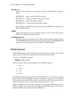
For example, the following statements print observations 20 through 25 of the data set FULL:
proc print data=full(firstobs=20 obs=25);
run;

Figure 3.3 Partial Listing of Data Set FULL
Obs date state i x y close
20 21OCT1993 NC 20 0.44803 0.35302 0.44803
21 22OCT1993 NC 21 0.03186 1.67414 0.03186
22 23OCT1993 NC 22 -0.25232 -1.61289 -0.25232
23 24OCT1993 NC 23 0.42524 0.73112 0.42524
24 25OCT1993 NC 24 0.05494 -0.88664 0.05494
25 26OCT1993 NC 25 -0.29096 -1.17275 -0.29096
You can use KEEP= and DROP= data set options to exclude variables from the input data set. See
SAS Language Reference: Dictionary for information about SAS data set options.
Storing Time Series in a SAS Data Set
This section discusses aspects of storing time series in SAS data sets. The topics discussed are the
standard form of a time series data set, storing several series with different time ranges in the same
data set, omitted observations, cross-sectional dimensions and BY groups, and interleaved time
series.
Any number of time series can be stored in a SAS data set. Normally, each time series is stored in a
separate variable. For example, the following statements augment the USCPI data set read in the
previous example with values for the producer price index:
data usprice;
input date : monyy7. cpi ppi;
format date monyy7.;
label cpi = "Consumer Price Index"
ppi = "Producer Price Index";
datalines;
76 ✦ Chapter 3: Working with Time Series Data
jun1990 129.9 114.3
jul1990 130.4 114.5
more lines
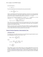
proc print data=usprice;
run;

Figure 3.4 Time Series Data Set Containing Two Series
Obs date cpi ppi
1 JUN1990 129.9 114.3
2 JUL1990 130.4 114.5
3 AUG1990 131.6 116.5
4 SEP1990 132.7 118.4
5 OCT1990 133.5 120.8
6 NOV1990 133.8 120.1
7 DEC1990 133.8 118.7
8 JAN1991 134.6 119.0
9 FEB1991 134.8 117.2
10 MAR1991 135.0 116.2
11 APR1991 135.2 116.0
12 MAY1991 135.6 116.5
13 JUN1991 136.0 116.3
14 JUL1991 136.2 116.0
Standard Form of a Time Series Data Set
The simple way the CPI and PPI time series are stored in the USPRICE data set in the preceding
example is termed the standard form of a time series data set. A time series data set in standard form
has the following characteristics:
 The data set contains one variable for each time series.
 The data set contains exactly one observation for each time period.

The data set contains an ID variable or variables that identify the time period of each observa-
tion.

The data set is sorted by the ID variables associated with date time values, so the observations
are in time sequence.

The data are equally spaced in time. That is, successive observations are a fixed time interval

apart, so the data set can be described by a single sampling interval such as hourly, daily,
monthly, quarterly, yearly, and so forth. This means that time series with different sampling
frequencies are not mixed in the same SAS data set.
Several Series with Different Ranges ✦ 77
Most SAS/ETS procedures that process time series expect the input data set to contain time series in
this standard form, and this is the simplest way to store time series in SAS data sets. (The EXPAND
and TIMESERIES procedures can be helpful in converting your data to this standard form.) There
are more complex ways to represent time series in SAS data sets.
You can incorporate cross-sectional dimensions with BY groups, so that each BY group is like
a standard form time series data set. This method is discussed in the section “Cross-Sectional
Dimensions and BY Groups” on page 79.
You can interleave time series, with several observations for each time period identified by another
ID variable. Interleaved time series data sets are used to store several series in the same SAS variable.
Interleaved time series data sets are often used to store series of actual values, predicted values, and
residuals, or series of forecast values and confidence limits for the forecasts. This is discussed in the
section “Interleaved Time Series” on page 80.
Several Series with Different Ranges
Different time series can have values recorded over different time ranges. Since a SAS data set must
have the same observations for all variables, when time series with different ranges are stored in the
same data set, missing values must be used for the periods in which a series is not available.
Suppose that in the previous example you did not record values for CPI before August 1990 and did
not record values for PPI after June 1991. The USPRICE data set could be read with the following
statements:
data usprice;
input date : monyy7. cpi ppi;
format date monyy7.;
datalines;
jun1990 . 114.3
jul1990 . 114.5
aug1990 131.6 116.5

sep1990 132.7 118.4
oct1990 133.5 120.8
nov1990 133.8 120.1
dec1990 133.8 118.7
jan1991 134.6 119.0
feb1991 134.8 117.2
mar1991 135.0 116.2
apr1991 135.2 116.0
may1991 135.6 116.5
jun1991 136.0 116.3
jul1991 136.2 .
;
The decimal points with no digits in the data records represent missing data and are read by SAS as
missing value codes.
78 ✦ Chapter 3: Working with Time Series Data
In this example, the time range of the USPRICE data set is June 1990 through July 1991, but the time
range of the CPI variable is August 1990 through July 1991, and the time range of the PPI variable is
June 1990 through June 1991.
SAS/ETS procedures ignore missing values at the beginning or end of a series. That is, the series is
considered to begin with the first nonmissing value and end with the last nonmissing value.
Missing Values and Omitted Observations
Missing data can also occur within a series. Missing values that appear after the beginning of a time
series and before the end of the time series are called embedded missing values.
Suppose that in the preceding example you did not record values for CPI for November 1990 and did
not record values for PPI for both November 1990 and March 1991. The USPRICE data set could be
read with the following statements:
data usprice;
input date : monyy. cpi ppi;
format date monyy.;
datalines;

jun1990 . 114.3
jul1990 . 114.5
aug1990 131.6 116.5
sep1990 132.7 118.4
oct1990 133.5 120.8
nov1990 . .
dec1990 133.8 118.7
jan1991 134.6 119.0
feb1991 134.8 117.2
mar1991 135.0 .
apr1991 135.2 116.0
may1991 135.6 116.5
jun1991 136.0 116.3
jul1991 136.2 .
;
In this example, the series CPI has one embedded missing value, and the series PPI has two embedded
missing values. The ranges of the two series are the same as before.
Note that the observation for November 1990 has missing values for both CPI and PPI; there is no
data for this period. This is an example of a missing observation.
You might ask why the data record for this period is included in the example at all, since the data
record contains no data. However, deleting the data record for November 1990 from the example
would cause an omitted observation in the USPRICE data set. SAS/ETS procedures expect input
data sets to contain observations for a contiguous time sequence. If you omit observations from
a time series data set and then try to analyze the data set with SAS/ETS procedures, the omitted
observations will cause errors. When all data are missing for a period, a missing observation should
be included in the data set to preserve the time sequence of the series.
Cross-Sectional Dimensions and BY Groups ✦ 79
If observations are omitted from the data set, the EXPAND procedure can be used to fill in the gaps
with missing values (or to interpolate nonmissing values) for the time series variables and with the
appropriate date or datetime values for the ID variable.

Cross-Sectional Dimensions and BY Groups
Often, time series in a collection are related by a cross sectional dimension. For example, the national
average U.S. consumer price index data shown in the previous example can be disaggregated to show
price indexes for major cities. In this case, there are several related time series: CPI for New York,
CPI for Chicago, CPI for Los Angeles, and so forth. When these time series are considered as one
data set, the city whose price level is measured is a cross sectional dimension of the data.
There are two basic ways to store such related time series in a SAS data set. The first way is to use a
standard form time series data set with a different variable for each series.
For example, the following statements read CPI series for three major U.S. cities:
data citycpi;
input date : monyy7. cpiny cpichi cpila;
format date monyy7.;
datalines;
nov1989 133.200 126.700 130.000
dec1989 133.300 126.500 130.600
more lines
The second way is to store the data in a time series cross-sectional form. In this form, the series
for all cross sections are stored in one variable and a cross section ID variable is used to identify
observations for the different series. The observations are sorted by the cross section ID variable and
by time within each cross section.
The following statements indicate how to read the CPI series for U.S. cities in time series cross-
sectional form:
data cpicity;
length city $11;
input city $11. date : monyy. cpi;
format date monyy.;
datalines;
New York JAN1990 135.100
New York FEB1990 135.300
more lines

proc sort data=cpicity;
by city date;
run;
80 ✦ Chapter 3: Working with Time Series Data
When processing a time series cross sectional form data set with most SAS/ETS procedures, use the
cross section ID variable in a BY statement to process the time series separately. The data set must
be sorted by the cross section ID variable and sorted by date within each cross section. The PROC
SORT step in the preceding example ensures that the CPICITY data set is correctly sorted.
When the cross section ID variable is used in a BY statement, each BY group in the data set is
like a standard form time series data set. Thus, SAS/ETS procedures that expect a standard form
time series data set can process time series cross sectional data sets when a BY statement is used,
producing an independent analysis for each cross section.
It is also possible to analyze time series cross-sectional data jointly. The PANEL procedure (and
the older TSCSREG procedure) expects the input data to be in the time series cross-sectional form
described here. See Chapter 19, “The PANEL Procedure,” for more information.
Interleaved Time Series
Normally, a time series data set has only one observation for each time period, or one observation for
each time period within a cross section for a time series cross-sectional-form data set. However, it is
sometimes useful to store several related time series in the same variable when the different series do
not correspond to levels of a cross-sectional dimension of the data.
In this case, the different time series can be interleaved. An interleaved time series data set is similar
to a time series cross-sectional data set, except that the observations are sorted differently and the ID
variable that distinguishes the different time series does not represent a cross-sectional dimension.
Some SAS/ETS procedures produce interleaved output data sets. The interleaved time series form
is a convenient way to store procedure output when the results consist of several different kinds of
series for each of several input series. (Interleaved time series are also easy to process with plotting
procedures. See the section “Plotting Time Series” on page 86.)
For example, the FORECAST procedure fits a model to each input time series and computes predicted
values and residuals from the model. The FORECAST procedure then uses the model to compute
forecast values beyond the range of the input data and also to compute upper and lower confidence

limits for the forecast values.
Thus, the output from PROC FORECAST consists of up to five related time series for each variable
forecast. The five resulting time series for each input series are stored in a single output variable with
the same name as the series that is being forecast. The observations for the five resulting series are
identified by values of the variable _TYPE_. These observations are interleaved in the output data
set with observations for the same date grouped together.
The following statements show how to use PROC FORECAST to forecast the variable CPI in the
USCPI data set. Figure 3.5 shows part of the output data set produced by PROC FORECAST and
illustrates the interleaved structure of this data set.
proc forecast data=uscpi interval=month lead=12
out=foreout outfull outresid;
var cpi;
Interleaved Time Series ✦ 81
id date;
run;
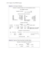
proc print data=foreout(obs=6);
run;
Figure 3.5 Partial Listing of Output Data Set Produced by PROC FORECAST
Obs date _TYPE_ _LEAD_ cpi
1 JUN1990 ACTUAL 0 129.900
2 JUN1990 FORECAST 0 130.817
3 JUN1990 RESIDUAL 0 -0.917
4 JUL1990 ACTUAL 0 130.400
5 JUL1990 FORECAST 0 130.678
6 JUL1990 RESIDUAL 0 -0.278
Observations with _TYPE_=ACTUAL contain the values of CPI read from the input data set.
Observations with _TYPE_=FORECAST contain one-step-ahead predicted values for observations
with dates in the range of the input series and contain forecast values for observations for dates
beyond the range of the input series. Observations with _TYPE_=RESIDUAL contain the difference
between the actual and one-step-ahead predicted values. Observations with _TYPE_=U95 and

_TYPE_=L95 contain the upper and lower bounds, respectively, of the 95% confidence interval for
the forecasts.
Using Interleaved Data Sets as Input to SAS/ETS Procedures
Interleaved time series data sets are not directly accepted as input by SAS/ETS procedures. However,
it is easy to use a WHERE statement with any procedure to subset the input data and select one of
the interleaved time series as the input.
For example, to analyze the residual series contained in the PROC FORECAST output data set with
another SAS/ETS procedure, include a WHERE _TYPE_=’RESIDUAL’ statement. The following
statements perform a spectral analysis of the residuals produced by PROC FORECAST in the
preceding example:
proc spectra data=foreout out=spectout;
var cpi;
where _type_='RESIDUAL';
run;
Combined Cross Sections and Interleaved Time Series Data Sets
Interleaved time series output data sets produced from BY-group processing of time series cross-
sectional input data sets have a complex structure that combines a cross-sectional dimension, a time
dimension, and the values of the _TYPE_ variable. For example, consider the PROC FORECAST
output data set produced by the following statements:
title "FORECAST Output Data Set with BY Groups";