SAS/ETS 9.22 User''''s Guide 28 pot

262 ✦ Chapter 7: The ARIMA Procedure
That is, the k-step forecast of x
tCk
, given .x
1
; ; x
t1
/, is
Qx
tCk
D C
k;t
V
1
t
.x
1
; ; x
t1
/
0
where
C
k;t
is the covariance of
x
tCk
and
.x
1
; ; x

t1
/
and
V
t
is the covariance matrix of the vector
.x
1
; ; x
t1
/. C
k;t
and V
t
are derived from the estimated parameters.
Finite memory forecasts minimize the mean squared error of prediction if the parameters of the
ARMA model are known exactly. (In most cases, the parameters of the ARMA model are estimated,
so the predictors are not true best linear forecasts.)
If the response series is differenced, the final forecast is produced by summing the forecast of the
differenced series. This summation and the forecast are conditional on the initial values of the series.
Thus, when the response series is differenced, the final forecasts are not true finite memory forecasts
because they are derived by assuming that the differenced series begins in a steady-state condition.
Thus, they fall somewhere between finite memory and infinite memory forecasts. In practice, there is
seldom any practical difference between these forecasts and true finite memory forecasts.
Forecasting Log Transformed Data
The log transformation is often used to convert time series that are nonstationary with respect to the
innovation variance into stationary time series. The usual approach is to take the log of the series in
a DATA step and then apply PROC ARIMA to the transformed data. A DATA step is then used to
transform the forecasts of the logs back to the original units of measurement. The confidence limits
are also transformed by using the exponential function.

As one alternative, you can simply exponentiate the forecast series. This procedure gives a forecast
for the median of the series, but the antilog of the forecast log series underpredicts the mean of the
original series. If you want to predict the expected value of the series, you need to take into account
the standard error of the forecast, as shown in the following example, which uses an AR(2) model to
forecast the log of a series Y:
data in;
set in;
ylog = log( y );
run;
proc arima data=in;
identify var=ylog;
estimate p=2;
forecast lead=10 out=out;
run;
data out;
set out;
y = exp( ylog );
l95 = exp( l95 );
u95 = exp( u95 );
forecast = exp( forecast + std
*
std/2 );
run;
Specifying Series Periodicity ✦ 263
Specifying Series Periodicity
The INTERVAL= option is used together with the ID= variable to describe the observations that make
up the time series. For example, INTERVAL=MONTH specifies a monthly time series in which
each observation represents one month. See Chapter 4, “Date Intervals, Formats, and Functions,” for
details about the interval values supported.
The variable specified by the ID= option in the PROC ARIMA statement identifies the time periods

associated with the observations. Usually, SAS date, time, or datetime values are used for this
variable. PROC ARIMA uses the ID= variable in the following ways:

to validate the data periodicity. When the INTERVAL= option is specified, PROC ARIMA
uses the ID variable to check the data and verify that successive observations have valid ID
values that correspond to successive time intervals. When the INTERVAL= option is not used,
PROC ARIMA verifies that the ID values are nonmissing and in ascending order.

to check for gaps in the input observations. For example, if INTERVAL=MONTH and an
input observation for April 1970 follows an observation for January 1970, there is a gap in
the input data with two omitted observations (namely February and March 1970). A warning
message is printed when a gap in the input data is found.

to label the forecast observations in the output data set. PROC ARIMA extrapolates the values
of the ID variable for the forecast observations from the ID value at the end of the input data
according to the frequency specifications of the INTERVAL= option. If the INTERVAL=
option is not specified, PROC ARIMA extrapolates the ID variable by incrementing the ID
variable value for the last observation in the input data by 1 for each forecast period. Values of
the ID variable over the range of the input data are copied to the output data set.
The ALIGN= option is used to align the ID variable to the beginning, middle, or end of the time ID
interval specified by the INTERVAL= option.
Detecting Outliers
You can use the OUTLIER statement to detect changes in the level of the response series that are not
accounted for by the estimated model. The types of changes considered are additive outliers (AO),
level shifts (LS), and temporary changes (TC).
Let
Á
t
be a regression variable that describes some type of change in the mean response. In time
series literature Á

t
is called a shock signature. An additive outlier at some time point s corresponds
to a shock signature
Á
t
such that
Á
s
D 1:0
and
Á
t
is 0.0 at all other points. Similarly a permanent
level shift that originates at time
s
has a shock signature such that
Á
t
is 0.0 for
t < s
and 1.0 for
t  s
. A temporary level shift of duration
d
that originates at time
s
has
Á
t
equal to 1.0 between

s
and s C d and 0.0 otherwise.
264 ✦ Chapter 7: The ARIMA Procedure
Suppose that you are estimating the ARIMA model
D.B/Y
t
D 
t
C
Â.B/
.B/
a
t
where
Y
t
is the response series,
D.B/
is the differencing polynomial in the backward shift operator B
(possibly identity),

t
is the transfer function input,
.B/
and
Â.B/
are the AR and MA polynomials,
respectively, and a
t
is the Gaussian white noise series.

The problem of detection of level shifts in the OUTLIER statement is formulated as a problem of
sequential selection of shock signatures that improve the model in the ESTIMATE statement. This is
similar to the forward selection process in the stepwise regression procedure. The selection process
starts with considering shock signatures of the type specified in the TYPE= option, originating at
each nonmissing measurement. This involves testing H
0
Wˇ D 0 versus H
a
Wˇ ¤ 0 in the model
D.B/.Y
t
 ˇÁ
t
/ D 
t
C
Â.B/
.B/
a
t
for each of these shock signatures. The most significant shock signature, if it also satisfies the
significance criterion in ALPHA= option, is included in the model. If no significant shock signature
is found, then the outlier detection process stops; otherwise this augmented model, which incorporates
the selected shock signature in its transfer function input, becomes the null model for the subsequent
selection process. This iterative process stops if at any stage no more significant shock signatures
are found or if the number of iterations exceeds the maximum search number that results due to the
MAXNUM= and MAXPCT= settings. In all these iterations, the parameters of the ARIMA model in
the ESTIMATE statement are held fixed.
The precise details of the testing procedure for a given shock signature Á
t

are as follows:
The preceding testing problem is equivalent to testing
H
0
Wˇ D 0
versus
H
a
Wˇ ¤ 0
in the following
“regression with ARMA errors” model
N
t
D ˇ
t
C
Â.B/
.B/
a
t
where
N
t
D .D.B/Y
t
 
t
/
is the “noise” process and


t
D D.B/Á
t
is the “effective” shock
signature.
In this setting, under
H
0
; N D .N
1
; N
2
; : : : ; N
n
/
T
is a mean zero Gaussian vector with variance
covariance matrix

2

. Here

2
is the variance of the white noise process
a
t
and

is the variance-

covariance matrix associated with the ARMA model. Moreover, under
H
a
,
N
has
ˇ
as the mean
vector where
 D .
1
; 
2
; : : : ; 
n
/
T
. Additionally, the generalized least squares estimate of
ˇ
and its
variance is given by
O
ˇ D ı=Ä
Var.
O
ˇ/ D 
2
=Ä
where
ı D 

T

1
N
and
Ä D 
T

1

. The test statistic

2
D ı
2
=.
2
Ä/
is used to test the
significance of
ˇ
, which has an approximate chi-squared distribution with 1 degree of freedom under
H
0
. The type of estimate of

2
used in the calculation of

2

can be specified by the SIGMA= option.
The default setting is SIGMA=ROBUST, which corresponds to a robust estimate suggested in an
OUT= Data Set ✦ 265
outlier detection procedure in X-12-ARIMA, the Census Bureau’s time series analysis program;
see Findley et al. (1998) for additional information. The robust estimate of

2
is computed by the
formula
O
2
D .1:49  Median.jOa
t
j//
2
where
Oa
t
are the standardized residuals of the null ARIMA model. The setting SIGMA=MSE
corresponds to the usual mean squared error estimate (MSE) computed the same way as in the
ESTIMATE statement with the NODF option.
The quantities
ı
and
Ä
are efficiently computed by a method described in de Jong and Penzer (1998);
see also Kohn and Ansley (1985).
Modeling in the Presence of Outliers
In practice, modeling and forecasting time series data in the presence of outliers is a difficult problem
for several reasons. The presence of outliers can adversely affect the model identification and

estimation steps. Their presence close to the end of the observation period can have a serious impact
on the forecasting performance of the model. In some cases, level shifts are associated with changes
in the mechanism that drives the observation process, and separate models might be appropriate
to different sections of the data. In view of all these difficulties, diagnostic tools such as outlier
detection and residual analysis are essential in any modeling process.
The following modeling strategy, which incorporates level shift detection in the familiar Box-Jenkins
modeling methodology, seems to work in many cases:
1.
Proceed with model identification and estimation as usual. Suppose this results in a tentative
ARIMA model, say M.
2.
Check for additive and permanent level shifts unaccounted for by the model M by using the
OUTLIER statement. In this step, unless there is evidence to justify it, the number of level
shifts searched should be kept small.
3.
Augment the original dataset with the regression variables that correspond to the detected
outliers.
4.
Include the first few of these regression variables in M, and call this model M1. Reestimate all
the parameters of M1. It is important not to include too many of these outlier variables in the
model in order to avoid the danger of over-fitting.
5.
Check the adequacy of M1 by examining the parameter estimates, residual analysis, and outlier
detection. Refine it more if necessary.
OUT= Data Set
The output data set produced by the OUT= option of the PROC ARIMA or FORECAST statements
contains the following:
266 ✦ Chapter 7: The ARIMA Procedure
 the BY variables
 the ID variable


the variable specified by the VAR= option in the IDENTIFY statement, which contains the
actual values of the response series

FORECAST, a numeric variable that contains the one-step-ahead predicted values and the
multistep forecasts
 STD, a numeric variable that contains the standard errors of the forecasts

a numeric variable that contains the lower confidence limits of the forecast. This variable is
named L95 by default but has a different name if the ALPHA= option specifies a different size
for the confidence limits.

RESIDUAL, a numeric variable that contains the differences between actual and forecast
values

a numeric variable that contains the upper confidence limits of the forecast. This variable is
named U95 by default but has a different name if the ALPHA= option specifies a different
size for the confidence limits.
The ID variable, the BY variables, and the response variable are the only ones copied from the input
to the output data set. In particular, the input variables are not copied to the OUT= data set.
Unless the NOOUTALL option is specified, the data set contains the whole time series. The
FORECAST variable has the one-step forecasts (predicted values) for the input periods, followed
by n forecast values, where n is the LEAD= value. The actual and RESIDUAL values are missing
beyond the end of the series.
If you specify the same OUT= data set in different FORECAST statements, the latter FORECAST
statements overwrite the output from the previous FORECAST statements. If you want to combine the
forecasts from different FORECAST statements in the same output data set, specify the OUT= option
once in the PROC ARIMA statement and omit the OUT= option in the FORECAST statements.
When a global output data set is created by the OUT= option in the PROC ARIMA statement, the
variables in the OUT= data set are defined by the first FORECAST statement that is executed. The

results of subsequent FORECAST statements are vertically concatenated onto the OUT= data set.
Thus, if no ID variable is specified in the first FORECAST statement that is executed, no ID variable
appears in the output data set, even if one is specified in a later FORECAST statement. If an ID
variable is specified in the first FORECAST statement that is executed but not in a later FORECAST
statement, the value of the ID variable is the same as the last value processed for the ID variable
for all observations created by the later FORECAST statement. Furthermore, even if the response
variable changes in subsequent FORECAST statements, the response variable name in the output
data set is that of the first response variable analyzed.
OUTCOV= Data Set ✦ 267
OUTCOV= Data Set
The output data set produced by the OUTCOV= option of the IDENTIFY statement contains the
following variables:

LAG, a numeric variable that contains the lags that correspond to the values of the covariance
variables. The values of LAG range from 0 to N for covariance functions and from –N to N
for cross-covariance functions, where N is the value of the NLAG= option.

VAR, a character variable that contains the name of the variable specified by the VAR= option.

CROSSVAR, a character variable that contains the name of the variable specified in the
CROSSCORR= option, which labels the different cross-covariance functions. The CROSS-
VAR variable is blank for the autocovariance observations. When there is no CROSSCORR=
option, this variable is not created.

N, a numeric variable that contains the number of observations used to calculate the current
value of the covariance or cross-covariance function.

COV, a numeric variable that contains the autocovariance or cross-covariance function values.
COV contains the autocovariances of the VAR= variable when the value of the CROSSVAR
variable is blank. Otherwise COV contains the cross covariances between the VAR= variable

and the variable named by the CROSSVAR variable.

CORR, a numeric variable that contains the autocorrelation or cross-correlation function
values. CORR contains the autocorrelations of the VAR= variable when the value of the
CROSSVAR variable is blank. Otherwise CORR contains the cross-correlations between the
VAR= variable and the variable named by the CROSSVAR variable.

STDERR, a numeric variable that contains the standard errors of the autocorrelations. The
standard error estimate is based on the hypothesis that the process that generates the time
series is a pure moving-average process of order LAG–1. For the cross-correlations, STDERR
contains the value
1=
p
n
, which approximates the standard error under the hypothesis that the
two series are uncorrelated.

INVCORR, a numeric variable that contains the inverse autocorrelation function values of the
VAR= variable. For cross-correlation observations (that is, when the value of the CROSSVAR
variable is not blank), INVCORR contains missing values.

PARTCORR, a numeric variable that contains the partial autocorrelation function values of the
VAR= variable. For cross-correlation observations (that is, when the value of the CROSSVAR
variable is not blank), PARTCORR contains missing values.
OUTEST= Data Set
PROC ARIMA writes the parameter estimates for a model to an output data set when the OUTEST=
option is specified in the ESTIMATE statement. The OUTEST= data set contains the following:
268 ✦ Chapter 7: The ARIMA Procedure
 the BY variables


_MODLABEL_, a character variable that contains the model label, if it is provided by using
the label option in the ESTIMATE statement (otherwise this variable is not created).

_NAME_, a character variable that contains the name of the parameter for the covariance or
correlation observations or is blank for the observations that contain the parameter estimates.
(This variable is not created if neither OUTCOV nor OUTCORR is specified.)

_TYPE_, a character variable that identifies the type of observation. A description of the
_TYPE_ variable values is given below.
 variables for model parameters
The variables for the model parameters are named as follows:
ERRORVAR
This numeric variable contains the variance estimate. The _TYPE_=EST obser-
vation for this variable contains the estimated error variance, and the remaining
observations are missing.
MU
This numeric variable contains values for the mean parameter for the model.
(This variable is not created if NOCONSTANT is specified.)
MAj _k
These numeric variables contain values for the moving-average parameters. The
variables for moving-average parameters are named MAj _k, where j is the
factor-number and k is the index of the parameter within a factor.
ARj _k
These numeric variables contain values for the autoregressive parameters. The
variables for autoregressive parameters are named ARj _k, where j is the factor
number and k is the index of the parameter within a factor.
Ij _k
These variables contain values for the transfer function parameters. Variables for
transfer function parameters are named Ij _k, where j is the number of the INPUT
variable associated with the transfer function component and k is the number of

the parameter for the particular INPUT variable. INPUT variables are numbered
according to the order in which they appear in the INPUT= list.
_STATUS_
This variable describes the convergence status of the model. A value of 0_CON-
VERGED indicates that the model converged.
The value of the _TYPE_ variable for each observation indicates the kind of value contained in the
variables for model parameters for the observation. The OUTEST= data set contains observations
with the following _TYPE_ values:
EST The observation contains parameter estimates.
STD The observation contains approximate standard errors of the estimates.
CORR
The observation contains correlations of the estimates. OUTCORR must be
specified to get these observations.
COV
The observation contains covariances of the estimates. OUTCOV must be speci-
fied to get these observations.
OUTEST= Data Set ✦ 269
FACTOR
The observation contains values that identify for each parameter the factor that
contains it. Negative values indicate denominator factors in transfer function
models.
LAG
The observation contains values that identify the lag associated with each param-
eter.
SHIFT
The observation contains values that identify the shift associated with the input
series for the parameter.
The values given for _TYPE_=FACTOR, _TYPE_=LAG, or _TYPE_=SHIFT observations enable
you to reconstruct the model employed when provided with only the OUTEST= data set.
OUTEST= Examples

This section clarifies how model parameters are stored in the OUTEST= data set with two examples.
Consider the following example:
proc arima data=input;
identify var=y cross=(x1 x2);
estimate p=(1)(6) q=(1,3)(12) input=(x1 x2) outest=est;
run;
proc print data=est;
run;
The model specified by these statements is
Y
t
D  C !
1;0
X
1;t
C !
2;0
X
2;t
C
.1  Â
11
B  Â
12
B
3
/.1  Â
21
B
12

/
.1  
11
B/.1  
21
B
6
/
a
t
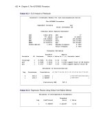
The OUTEST= data set contains the values shown in Table 7.10.
Table 7.10 OUTEST= Data Set for First Example
Obs _TYPE_ Y MU MA1_1 MA1_2 MA2_1 AR1_1 AR2_1 I1_1 I2_1
1 EST 
2
 Â
11
Â
12
Â
21

11

21
!
1;0
!
2;0
2 STD . se  se Â

11
se Â
12
se Â
21
se 
11
se 
21
se !
1;0
se !
2;0
3 FACTOR . 0 1 1 2 1 2 1 1
4 LAG . 0 1 3 12 1 6 0 0
5 SHIFT . 0 0 0 0 0 0 0 0
Note that the symbols in the rows for _TYPE_=EST and _TYPE_=STD in Table 7.10 would be
numeric values in a real data set.
Next, consider the following example:
proc arima data=input;
identify var=y cross=(x1 x2);
270 ✦ Chapter 7: The ARIMA Procedure
estimate p=1 q=1 input=(2 $ (1)/(1,2)x1 1 $ /(1)x2) outest=est;
run;
proc print data=est;
run;
The model specified by these statements is
Y
t
D  C

!
10
 !
11
B
1  ı
11
B  ı
12
B
2
X
1;t2
C
!
20
1  ı
21
B
X
2;t1
C
.1  Â
1
B/
.1  
1
B/
a
t

The OUTEST= data set contains the values shown in Table 7.11.
Table 7.11 OUTEST= Data Set for Second Example
Obs _TYPE_ Y MU MA1_1 AR1_1 I1_1 I1_2 I1_3 I1_4 I2_1 I2_2
1 EST 
2
 Â
1

1
!
10
!
11
ı
11
ı
12
!
20
ı
21
2 STD . se  se Â
1
se 
1
se !
10
se !
11
se ı

11
se ı
12
se !
20
se ı
21
3 FACTOR . 0 1 1 1 1 -1 -1 1 -1
4 LAG . 0 1 1 0 1 1 2 0 1
5 SHIFT . 0 0 0 2 2 2 2 1 1
OUTMODEL= SAS Data Set
The OUTMODEL= option in the ESTIMATE statement writes an output data set that enables you
to reconstruct the model. The OUTMODEL= data set contains much the same information as the
OUTEST= data set but in a transposed form that might be more useful for some purposes. In addition,
the OUTMODEL= data set includes the differencing operators.
The OUTMODEL data set contains the following:
 the BY variables

_MODLABEL_, a character variable that contains the model label, if it is provided by using
the label option in the ESTIMATE statement (otherwise this variable is not created).

_NAME_, a character variable that contains the name of the response or input variable for the
observation.

_TYPE_, a character variable that contains the estimation method that was employed. The
value of _TYPE_ can be CLS, ULS, or ML.

_STATUS_, a character variable that describes the convergence status of the model. A value
of 0_CONVERGED indicates that the model converged.


_PARM_, a character variable that contains the name of the parameter given by the observation.
_PARM_ takes on the values ERRORVAR, MU, AR, MA, NUM, DEN, and DIF.
OUTMODEL= SAS Data Set ✦ 271

_VALUE_, a numeric variable that contains the value of the estimate defined by the _PARM_
variable.
 _STD_, a numeric variable that contains the standard error of the estimate.

_FACTOR_, a numeric variable that indicates the number of the factor to which the parameter
belongs.

_LAG_, a numeric variable that contains the number of the term within the factor that contains
the parameter.

_SHIFT_, a numeric variable that contains the shift value for the input variable associated
with the current parameter.
The values of _FACTOR_ and _LAG_ identify which particular MA, AR, NUM, or DEN parameter
estimate is given by the _VALUE_ variable. The _NAME_ variable contains the response variable
name for the MU, AR, or MA parameters. Otherwise, _NAME_ contains the input variable name
associated with NUM or DEN parameter estimates. The _NAME_ variable contains the appropriate
variable name associated with the current DIF observation as well. The _VALUE_ variable is 1 for
all DIF observations, and the _LAG_ variable indicates the degree of differencing employed.
The observations contained in the OUTMODEL= data set are identified by the _PARM_ variable. A
description of the values of the _PARM_ variable follows:
NUMRESID _VALUE_ contains the number of residuals.
NPARMS _VALUE_ contains the number of parameters in the model.
NDIFS
_VALUE_ contains the sum of the differencing lags employed for the response
variable.
ERRORVAR _VALUE_ contains the estimate of the innovation variance.

MU _VALUE_ contains the estimate of the mean term.
AR
_VALUE_ contains the estimate of the autoregressive parameter indexed by the
_FACTOR_ and _LAG_ variable values.
MA
_VALUE_ contains the estimate of a moving-average parameter indexed by the
_FACTOR_ and _LAG_ variable values.
NUM
_VALUE_ contains the estimate of the parameter in the numerator factor of the
transfer function of the input variable indexed by the _FACTOR_, _LAG_, and
_SHIFT_ variable values.
DEN
_VALUE_ contains the estimate of the parameter in the denominator factor of the
transfer function of the input variable indexed by the _FACTOR_, _LAG_, and
_SHIFT_ variable values.
DIF
_VALUE_ contains the difference operator defined by the difference lag given by
the value in the _LAG_ variable.