SAS/ETS 9.22 User''''s Guide 14 potx

122 ✦ Chapter 3: Working with Time Series Data
By default, the EXPAND procedure performs interpolation by first fitting cubic spline curves to the
available data and then computing needed interpolating values from the fitted spline curves. Other
interpolation methods can be requested.
Note that interpolating values of a time series does not add any real information to the data because
the interpolation process is not the same process that generated the other (nonmissing) values in the
series. While time series interpolation can sometimes be useful, great care is needed in analyzing
time series that contain interpolated values.
Interpolating Missing Values
To use the EXPAND procedure to interpolate missing values in a time series, specify the input
and output data sets in the PROC EXPAND statement, and specify the time ID variable in an ID
statement. For example, the following statements cause PROC EXPAND to interpolate values for
missing values of all numeric variables in the data set USPRICE:
proc expand data=usprice out=interpl;
id date;
run;
Interpolated values are computed only for embedded missing values in the input time series. Missing
values before or after the range of a series are ignored by the EXPAND procedure.
In the preceding example, PROC EXPAND assumes that all series are measured at points in time
given by the value of the ID variable. In fact, the series in the USPRICE data set are monthly averages.
PROC EXPAND can produce a better interpolation if this is taken into account. The following
example uses the FROM=MONTH option to tell PROC EXPAND that the series is monthly and uses
the CONVERT statement with the OBSERVED=AVERAGE to specify that the series values are
averages over each month:
proc expand data=usprice out=interpl
from=month;
id date;
convert cpi ppi / observed=average;
run;
Interpolating to a Higher or Lower Frequency
You can use PROC EXPAND to interpolate values of time series at a higher or lower sampling

frequency than the input time series. To change the periodicity of time series, specify the time
interval of the input data set with the FROM= option, and specify the time interval for the desired
output frequency with the TO= option. For example, the following statements compute interpolated
weekly values of the monthly CPI and PPI series:
proc expand data=usprice out=interpl
Interpolating between Stocks and Flows, Levels and Rates ✦ 123
from=month to=week;
id date;
convert cpi ppi / observed=average;
run;
Interpolating between Stocks and Flows, Levels and Rates
A distinction is made between variables that are measured at points in time and variables that
represent totals or averages over an interval. Point-in-time values are often called stocks or levels.
Variables that represent totals or averages over an interval are often called flows or rates.
For example, the annual series Gross National Product represents the final goods production of over
the year and also the yearly average rate of that production. However, the monthly variable Inventory
represents the cost of a stock of goods at the end of the month.
The EXPAND procedure can convert between point-in-time values and period average or total
values. To convert observation characteristics, specify the input and output characteristics with the
OBSERVED= option in the CONVERT statement. For example, the following statements use the
monthly average price index values in USPRICE to compute interpolated estimates of the price index
levels at the midpoint of each month.
proc expand data=usprice out=midpoint
from=month;
id date;
convert cpi ppi / observed=(average,middle);
run;
Reading Time Series Data
Time series data can be coded in many different ways. The SAS System can read time series data
recorded in almost any form. Earlier sections of this chapter show how to read time series data coded

in several commonly used ways. This section shows how to read time series data from data records
coded in two other commonly used ways not previously introduced.
Several time series databases distributed by major data vendors can be read into SAS data sets by the
DATASOURCE procedure. See Chapter 11, “The DATASOURCE Procedure,” for more information.
The SASECRSP, SASEFAME, and SASEHAVR interface engines enable SAS users to access and
process time series data in CRSPAccess data files, FAME databases, and Haver Analytics Data
Link Express (DLX) data bases, respectively. See Chapter 35, “The SASECRSP Interface Engine,”
Chapter 36, “The SASEFAME Interface Engine,” and Chapter 37, “The SASEHAVR Interface
Engine,” for more details.
124 ✦ Chapter 3: Working with Time Series Data
Reading a Simple List of Values
Time series data can be coded as a simple list of values without dating information and with an
arbitrary number of observations on each data record. In this case, the INPUT statement must use the
trailing “@@” option to retain the current data record after reading the values for each observation,
and the time ID variable must be generated with programming statements.
For example, the following statements read the USPRICE data set from data records that contain
pairs of values for CPI and PPI. This example assumes you know that the first pair of values is for
June 1990.
data usprice;
input cpi ppi @@;
date = intnx( 'month', '1jun1990'd, _n_-1 );
format date monyy7.;
datalines;
129.9 114.3 130.4 114.5 131.6 116.5
132.7 118.4 133.5 120.8 133.8 120.1 133.8 118.7
134.6 119.0 134.8 117.2 135.0 116.2 135.2 116.0
135.6 116.5 136.0 116.3 136.2 116.0
;
Reading Fully Described Time Series in Transposed Form
Data for several time series can be coded with separate groups of records for each time series. Data

files coded this way are transposed from the form required by SAS procedures. Time series data can
also be coded with descriptive information about the series included with the data records.
The following example reads time series data for the USPRICE data set coded with separate groups
of records for each series. The data records for each series consist of a series description record and
one or more value records. The series description record gives the series name, starting month and
year of the series, number of values in the series, and a series label. The value records contain the
observations of the time series.
The data are first read into a temporary data set that contains one observation for each value of each
series.
data temp;
length _name_ $8 _label_ $40;
keep _name_ _label_ date value;
format date monyy.;
input _name_ month year nval _label_ &;
date = mdy( month, 1, year );
do i = 1 to nval;
input value @;
output;
date = intnx( 'month', date, 1 );
end;
Reading Fully Described Time Series in Transposed Form ✦ 125
datalines;
cpi 8 90 12 Consumer Price Index
131.6 132.7 133.5 133.8 133.8 134.6 134.8 135.0
135.2 135.6 136.0 136.2
ppi 6 90 13 Producer Price Index
114.3 114.5 116.5 118.4 120.8 120.1 118.7 119.0
117.2 116.2 116.0 116.5 116.3
;
The following statements sort the data set by date and series name, and the TRANSPOSE procedure

is used to transpose the data into a standard form time series data set.
proc sort data=temp;
by date _name_;
run;
proc transpose data=temp out=usprice(drop=_name_);
by date;
var value;
run;
proc contents data=usprice;
run;
proc print data=usprice;
run;
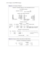
The final data set is shown in Figure 3.25.
Figure 3.24 Contents of USPRICE Data Set
Retransposed Data Set
The CONTENTS Procedure
Alphabetic List of Variables and Attributes
# Variable Type Len Format Label
3 cpi Num 8 Consumer Price Index
1 date Num 8 MONYY.
2 ppi Num 8 Producer Price Index
126 ✦ Chapter 3: Working with Time Series Data
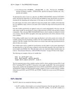
Figure 3.25 Listing of USPRICE Data Set
Retransposed Data Set
Obs date ppi cpi
1 JUN90 114.3 .
2 JUL90 114.5 .
3 AUG90 116.5 131.6
4 SEP90 118.4 132.7
5 OCT90 120.8 133.5

6 NOV90 120.1 133.8
7 DEC90 118.7 133.8
8 JAN91 119.0 134.6
9 FEB91 117.2 134.8
10 MAR91 116.2 135.0
11 APR91 116.0 135.2
12 MAY91 116.5 135.6
13 JUN91 116.3 136.0
14 JUL91 . 136.2
Chapter 4
Date Intervals, Formats, and Functions
Contents
Overview . . . . . . . . . . . . . . . . . . . . . . . . . . . . . . . . . . . . . . . . 127
Time Intervals . . . . . . . . . . . . . . . . . . . . . . . . . . . . . . . . . . . . . 128
Constructing Interval Names . . . . . . . . . . . . . . . . . . . . . . . . . . 128
Shifted Intervals . . . . . . . . . . . . . . . . . . . . . . . . . . . . . . . . 129
Beginning Dates and Datetimes of Intervals . . . . . . . . . . . . . . . . . . 130
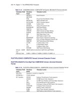
Summary of Interval Types . . . . . . . . . . . . . . . . . . . . . . . . . . . 131
Examples of Interval Specifications . . . . . . . . . . . . . . . . . . . . . . 134
Custom Time Intervals . . . . . . . . . . . . . . . . . . . . . . . . . . . . . . . . 135
Date and Datetime Informats . . . . . . . . . . . . . . . . . . . . . . . . . . . . . 140
Date, Time, and Datetime Formats . . . . . . . . . . . . . . . . . . . . . . . . . . . 141
Date Formats . . . . . . . . . . . . . . . . . . . . . . . . . . . . . . . . . . 142
Datetime and Time Formats . . . . . . . . . . . . . . . . . . . . . . . . . . 146
Alignment of SAS Dates . . . . . . . . . . . . . . . . . . . . . . . . . . . . . . . 146
SAS Date, Time, and Datetime Functions . . . . . . . . . . . . . . . . . . . . . . . 147
References . . . . . . . . . . . . . . . . . . . . . . . . . . . . . . . . . . . . . . 152
Overview
This chapter summarizes the time intervals, date and datetime informats, date and datetime formats,
and date, time, and datetime functions available in SAS software. The use of these features is ex-

plained in Chapter 3, “Working with Time Series Data.” The material in this chapter is also contained
in SAS Language Reference: Concepts and SAS Language Reference: Dictionary. Because these
features are useful for work with time series data, documentation of these features is consolidated
and repeated here for easy reference.
128 ✦ Chapter 4: Date Intervals, Formats, and Functions
Time Intervals
This section provides a reference for the different kinds of time intervals supported by SAS software,
but it does not cover how they are used. For an introduction to the use of time intervals, see Chapter 3,
“Working with Time Series Data.”
Some interval names are used with SAS date values, while other interval names are used with
SAS datetime values. The interval names used with SAS date values are YEAR, SEMIYEAR,
QTR, MONTH, SEMIMONTH, TENDAY, WEEK, WEEKDAY, DAY, YEARV, R445YR, R454YR,
R544YR, R445QTR, R454QTR, R544QTR, R445MON, R454MON, R544MON, and WEEKV. The
interval names used with SAS datetime or time values are HOUR, MINUTE, and SECOND. Various
abbreviations of these names are also allowed, as described in the section “Summary of Interval
Types” on page 131.
Interval names for use with SAS date values can be prefixed with ‘DT’ to construct interval
names for use with SAS datetime values. The interval names DTYEAR, DTSEMIYEAR, DTQTR,
DTMONTH, DTSEMIMONTH, DTTENDAY, DTWEEK, DTWEEKDAY, DTDAY, DTYEARV,
DTR445YR, DTR454YR, DTR544YR, DTR445QTR, DTR454QTR, DTR544QTR, DTR445MON,
DTR454MON, DTR544MON, and DTWEEKV are used with SAS datetime values.
Constructing Interval Names
Multipliers and shift indexes can be used with the basic interval names to construct more complex
interval specifications. The general form of an interval name is as follows:
NAMEn.s
The three parts of the interval name are shown below:
NAME
the name of the basic interval type. For example, YEAR specifies yearly
intervals.
n

an optional multiplier that specifies that the interval is a multiple of the
period of the basic interval type. For example, the interval YEAR2 consists
of two-year (biennial) periods.
s
an optional starting subperiod index that specifies that the intervals are shifted
to later starting points. For example, YEAR.3 specifies yearly periods shifted
to start on the first of March of each calendar year and to end in February of
the following year.
Both the multiplier n and the shift index s are optional and default to 1. For example, YEAR, YEAR1,
YEAR.1, and YEAR1.1 are all equivalent ways of specifying ordinary calendar years.
Shifted Intervals ✦ 129
To test for a valid interval specification, use the INTTEST function:
interval = 'MONTH3.2';
valid = INTTEST( interval );
valid = INTTEST( 'YEAR4');
INTTEST returns a value of 0 if the argument is not a valid interval specification and 1 if the
argument is a valid interval specification. The INTTEST function can also be used in a DATA step to
test an interval before calling an interval function:
valid = INTTEST( interval );
if ( valid = 1 ) then do;
end_date = INTNX( interval, date, 0, 'E' );
Status = 'Success';
end;
if ( valid = 0 ) then Status = 'Failure';
For more information about the INTTEST function, see the SAS Language Reference: Dictionary.
Shifted Intervals
Different kinds of intervals are shifted by different subperiods:
 YEAR, SEMIYEAR, QTR, and MONTH intervals are shifted by calendar months.
 WEEK and DAY intervals are shifted by days.
 SEMIMONTH intervals are shifted by semimonthly periods.

 TENDAY intervals are shifted by 10-day periods.
 YEARV intervals are shifted by WEEKV intervals.
 R445YR, R445QTR, and R445MON intervals are shifted by R445MON intervals.
 R454YR, R454QTR, and R454MON intervals are shifted by R454MON intervals.
 R544YR, R544QTR, and R544MON intervals are shifted by R544MON intervals.
 WEEKV intervals are shifted by days.
 WEEKDAY intervals are shifted by weekdays.
 HOUR intervals are shifted by hours.
 MINUTE intervals are shifted by minutes.
 SECOND intervals are shifted by seconds.
130 ✦ Chapter 4: Date Intervals, Formats, and Functions
The INTSHIFT function returns the shift interval:
interval = 'MONTH3.2';
shift_interval = INTSHIFT( interval );
In this example, the value of shift_interval is ‘MONTH’. For more information about the INTSHIFT
function, see the SAS Language Reference: Dictionary.
If a subperiod is specified, the shift index cannot be greater than the number of subperiods in the
whole interval. For example, you can use YEAR2.24, but YEAR2.25 is an error because there is no
25th month in a two-year interval.
For interval types that shift by subperiods that are the same as the basic interval type, only multiperiod
intervals can be shifted. For example, MONTH type intervals shift by MONTH subintervals; thus,
monthly intervals cannot be shifted because there is only one month in MONTH. However, bimonthly
intervals can be shifted because there are two MONTH intervals in each MONTH2 interval. The
interval name MONTH2.2 specifies bimonthly periods that start on the first day of even-numbered
months.
Beginning Dates and Datetimes of Intervals
Intervals that represent divisions of a year begin with the start of the year (1 January). YEARV,
R445YR, R454YR, and R544YR intervals begin with the first week of the International Organization
for Standardization (ISO) year, the Monday on or immediately preceding January
4

th. R445QTR,
R454QTR, and R544QTR intervals begin with the
1
st,
14
th,
27
th, and
40
th weeks of the ISO year.
MONTH2 periods begin with odd-numbered months (January, March, May, and so on).
Likewise, intervals that represent divisions of a day begin with the start of the day (midnight). Thus,
HOUR8.7 intervals divide the day into the periods 06:00 to 14:00, 14:00 to 22:00, and 22:00 to
06:00.
Intervals that do not nest within years or days begin relative to the SAS date or datetime value 0. The
arbitrary reference time of midnight on January 1, 1960, is used as the origin for nonshifted intervals,
and shifted intervals are defined relative to that reference point. For example, MONTH13 defines the
intervals January 1, 1960, February 1, 1961, March 1, 1962, and so forth, and the intervals December
1, 1959, November 1, 1958, and so on before the base date January 1, 1960.
Similarly, the WEEK2 interval begins relative to the Sunday of the week of January 1, 1960. The
interval specification WEEK6.13 defines six-week periods that start on second Fridays, and the
convention of counting relative to the period that contains January 1, 1960, indicates the starting
date or datetime of the interval closest to January 1, 1960, that corresponds to the second Fridays of
six-week intervals.
Intervals always begin on the date or datetime defined by the base interval name, the multiplier,
and the shift value. The end of the interval immediately precedes the beginning of the next interval.
However, an interval can be identified by any date or datetime value between its starting and ending
values, inclusive. See the section “Alignment of SAS Dates” on page 146 for more information about
generating identifying dates for intervals.
Summary of Interval Types ✦ 131

Summary of Interval Types
The interval types are summarized as follows:
YEAR
specifies yearly intervals. Abbreviations are YEAR, YEARS, YEARLY, YR, ANNUAL,
ANNUALLY, and ANNUALS. The starting subperiod s is in months (MONTH).
YEARV
specifies ISO 8601 yearly intervals. The ISO 8601 year starts on the Monday on or immediately
preceding January
4
th. Note that it is possible for the ISO 8601 year to start in December of the
preceding year. Also, some ISO 8601 years contain a leap week. For further discussion of ISO
weeks, see Technical Committee ISO/TC 154, Documents in Commerce, and Administration
(2004). The starting subperiod s is in ISO 8601 weeks (WEEKV).
R445YR
is the same as YEARV except that the starting subperiod s is in retail 4-4-5 months
(R445MON).
R454YR
is the same as YEARV except that the starting subperiod s is in retail 4-5-4 months (R454MON).
For a discussion of the retail 4-5-4 calendar, see National Retail Federation (2007).
R544YR
is the same as YEARV except that the starting subperiod s is in retail 5-4-4 months
(R544MON).
SEMIYEAR
specifies semiannual intervals (every six months). Abbreviations are SEMIYEAR,
SEMIYEARS, SEMIYEARLY, SEMIYR, SEMIANNUAL, and SEMIANN.
The starting subperiod s is in months (MONTH). For example, SEMIYEAR.3 intervals are
March–August and September–February.
QTR
specifies quarterly intervals (every three months). Abbreviations are QTR, QUARTER, QUAR-
TERS, QUARTERLY, QTRLY, and QTRS. The starting subperiod s is in months (MONTH).

R445QTR
specifies retail 4-4-5 quarterly intervals (every 13 ISO 8601 weeks). Some fourth quarters
contain a leap week. The starting subperiod s is in retail 4-4-5 months (R445MON).
R454QTR
specifies retail 4-5-4 quarterly intervals (every 13 ISO 8601 weeks). Some fourth quarters
contain a leap week. For a discussion of the retail 4-5-4 calendar, see National Retail Federation
(2007). The starting subperiod s is in retail 4-5-4 months (R454MON).
R544QTR
specifies retail 5-4-4 quarterly intervals (every 13 ISO 8601 weeks). Some fourth quarters
contain a leap week. The starting subperiod s is in retail 5-4-4 months (R544MON).