SAS/ETS 9.22 User''''s Guide 44 potx

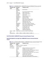
422 ✦ Chapter 8: The AUTOREG Procedure
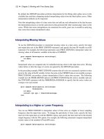
Output 8.2.1 OLS Analysis of Residuals
Grunfeld's Investment Models Fit with Autoregressive Errors
The AUTOREG Procedure
Dependent Variable gei
Gross investment GE
Ordinary Least Squares Estimates
SSE 13216.5878 DFE 17
MSE 777.44634 Root MSE 27.88272
SBC 195.614652 AIC 192.627455
MAE 19.9433255 AICC 194.127455
MAPE 23.2047973 HQC 193.210587
Durbin-Watson 1.0721 Regress R-Square 0.7053
Total R-Square 0.7053
Parameter Estimates
Standard Approx
Variable DF Estimate Error t Value Pr > |t| Variable Label
Intercept 1 -9.9563 31.3742 -0.32 0.7548
gef 1 0.0266 0.0156 1.71 0.1063 Lagged Value of GE shares
gec 1 0.1517 0.0257 5.90 <.0001 Lagged Capital Stock GE
Estimates of Autocorrelations
Lag Covariance Correlation -1 9 8 7 6 5 4 3 2 1 0 1 2 3 4 5 6 7 8 9 1
0 660.8 1.000000 | |
********************
|
1 304.6 0.460867 | |
*********
|
Preliminary MSE 520.5
Output 8.2.2 Regression Results Using Default Yule-Walker Method
Estimates of Autoregressive Parameters

Standard
Lag Coefficient Error t Value
1 -0.460867 0.221867 -2.08
Example 8.2: Comparing Estimates and Models ✦ 423
Output 8.2.2 continued
Yule-Walker Estimates
SSE 10238.2951 DFE 16
MSE 639.89344 Root MSE 25.29612
SBC 193.742396 AIC 189.759467
MAE 18.0715195 AICC 192.426133
MAPE 21.0772644 HQC 190.536976
Durbin-Watson 1.3321 Regress R-Square 0.5717
Total R-Square 0.7717
Parameter Estimates
Standard Approx
Variable DF Estimate Error t Value Pr > |t| Variable Label
Intercept 1 -18.2318 33.2511 -0.55 0.5911
gef 1 0.0332 0.0158 2.10 0.0523 Lagged Value of GE shares
gec 1 0.1392 0.0383 3.63 0.0022 Lagged Capital Stock GE
Output 8.2.3 Regression Results Using Unconditional Least Squares Method
Estimates of Autoregressive Parameters
Standard
Lag Coefficient Error t Value
1 -0.460867 0.221867 -2.08
Algorithm converged.
Unconditional Least Squares Estimates
SSE 10220.8455 DFE 16
MSE 638.80284 Root MSE 25.27455
SBC 193.756692 AIC 189.773763
MAE 18.1317764 AICC 192.44043

MAPE 21.149176 HQC 190.551273
Durbin-Watson 1.3523 Regress R-Square 0.5511
Total R-Square 0.7721
Parameter Estimates
Standard Approx
Variable DF Estimate Error t Value Pr > |t| Variable Label
Intercept 1 -18.6582 34.8101 -0.54 0.5993
gef 1 0.0339 0.0179 1.89 0.0769 Lagged Value of GE shares
gec 1 0.1369 0.0449 3.05 0.0076 Lagged Capital Stock GE
AR1 1 -0.4996 0.2592 -1.93 0.0718
424 ✦ Chapter 8: The AUTOREG Procedure
Output 8.2.3 continued
Autoregressive parameters assumed given
Standard Approx
Variable DF Estimate Error t Value Pr > |t| Variable Label
Intercept 1 -18.6582 33.7567 -0.55 0.5881
gef 1 0.0339 0.0159 2.13 0.0486 Lagged Value of GE shares
gec 1 0.1369 0.0404 3.39 0.0037 Lagged Capital Stock GE
Output 8.2.4 Regression Results Using Maximum Likelihood Method
Estimates of Autoregressive Parameters
Standard
Lag Coefficient Error t Value
1 -0.460867 0.221867 -2.08
Algorithm converged.
Maximum Likelihood Estimates
SSE 10229.2303 DFE 16
MSE 639.32689 Root MSE 25.28491
SBC 193.738877 AIC 189.755947
MAE 18.0892426 AICC 192.422614
MAPE 21.0978407 HQC 190.533457

Durbin-Watson 1.3385 Regress R-Square 0.5656
Total R-Square 0.7719
Parameter Estimates
Standard Approx
Variable DF Estimate Error t Value Pr > |t| Variable Label
Intercept 1 -18.3751 34.5941 -0.53 0.6026
gef 1 0.0334 0.0179 1.87 0.0799 Lagged Value of GE shares
gec 1 0.1385 0.0428 3.23 0.0052 Lagged Capital Stock GE
AR1 1 -0.4728 0.2582 -1.83 0.0858
Autoregressive parameters assumed given
Standard Approx
Variable DF Estimate Error t Value Pr > |t| Variable Label
Intercept 1 -18.3751 33.3931 -0.55 0.5897
gef 1 0.0334 0.0158 2.11 0.0512 Lagged Value of GE shares
gec 1 0.1385 0.0389 3.56 0.0026 Lagged Capital Stock GE
Example 8.3: Lack-of-Fit Study ✦ 425
Example 8.3: Lack-of-Fit Study
Many time series exhibit high positive autocorrelation, having the smooth appearance of a random
walk. This behavior can be explained by the partial adjustment and adaptive expectation hypotheses.
Short-term forecasting applications often use autoregressive models because these models absorb
the behavior of this kind of data. In the case of a first-order AR process where the autoregressive
parameter is exactly 1 (a random walk ), the best prediction of the future is the immediate past.
PROC AUTOREG can often greatly improve the fit of models, not only by adding additional
parameters but also by capturing the random walk tendencies. Thus, PROC AUTOREG can be
expected to provide good short-term forecast predictions.
However, good forecasts do not necessarily mean that your structural model contributes anything
worthwhile to the fit. In the following example, random noise is fit to part of a sine wave. Notice
that the structural model does not fit at all, but the autoregressive process does quite well and is
very nearly a first difference (AR(1) =
:976

). The DATA step, PROC AUTOREG step, and PROC
SGPLOT step follow:
title1 'Lack of Fit Study';
title2 'Fitting White Noise Plus Autoregressive Errors to a Sine Wave';
data a;
pi=3.14159;
do time = 1 to 75;
if time > 75 then y = .;
else y = sin( pi
*
( time / 50 ) );
x = ranuni( 1234567 );
output;
end;
run;
proc autoreg data=a plots;
model y = x / nlag=1;
output out=b p=pred pm=xbeta;
run;
proc sgplot data=b;
scatter y=y x=time / markerattrs=(color=black);
series y=pred x=time / lineattrs=(color=blue);
series y=xbeta x=time / lineattrs=(color=red);
run;
The printed output produced by PROC AUTOREG is shown in Output 8.3.1 and Output 8.3.2.
Plots of observed and predicted values are shown in Output 8.3.3 and Output 8.3.4. Note: the
plot Output 8.3.3 can be viewed in the Autoreg.Model.FitDiagnosticPlots category by selecting
ViewIResults.
426 ✦ Chapter 8: The AUTOREG Procedure
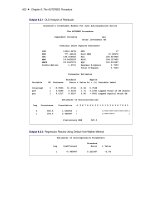
Output 8.3.1 Results of OLS Analysis: No Autoregressive Model Fit

Lack of Fit Study
Fitting White Noise Plus Autoregressive Errors to a Sine Wave
The AUTOREG Procedure
Dependent Variable y
Ordinary Least Squares Estimates
SSE 34.8061005 DFE 73
MSE 0.47680 Root MSE 0.69050
SBC 163.898598 AIC 159.263622
MAE 0.59112447 AICC 159.430289
MAPE 117894.045 HQC 161.114317
Durbin-Watson 0.0057 Regress R-Square 0.0008
Total R-Square 0.0008
Parameter Estimates
Standard Approx
Variable DF Estimate Error t Value Pr > |t|
Intercept 1 0.2383 0.1584 1.50 0.1367
x 1 -0.0665 0.2771 -0.24 0.8109
Estimates of Autocorrelations
Lag Covariance Correlation -1 9 8 7 6 5 4 3 2 1 0 1 2 3 4 5 6 7 8 9 1
0 0.4641 1.000000 | |
********************
|
1 0.4531 0.976386 | |
********************
|
Preliminary MSE 0.0217
Output 8.3.2 Regression Results with AR(1) Error Correction
Estimates of Autoregressive Parameters
Standard
Lag Coefficient Error t Value

1 -0.976386 0.025460 -38.35
Yule-Walker Estimates
SSE 0.18304264 DFE 72
MSE 0.00254 Root MSE 0.05042
SBC -222.30643 AIC -229.2589
MAE 0.04551667 AICC -228.92087
MAPE 29145.3526 HQC -226.48285
Durbin-Watson 0.0942 Regress R-Square 0.0001
Total R-Square 0.9947
Example 8.3: Lack-of-Fit Study ✦ 427
Output 8.3.2 continued
Parameter Estimates
Standard Approx
Variable DF Estimate Error t Value Pr > |t|
Intercept 1 -0.1473 0.1702 -0.87 0.3898
x 1 -0.001219 0.0141 -0.09 0.9315
Output 8.3.3 Diagnostics Plots
428 ✦ Chapter 8: The AUTOREG Procedure
Output 8.3.4 Plot of Autoregressive Prediction
Example 8.4: Missing Values ✦ 429
Example 8.4: Missing Values
In this example, a pure autoregressive error model with no regressors is used to generate 50 values
of a time series. Approximately 15% of the values are randomly chosen and set to missing. The
following statements generate the data:
title 'Simulated Time Series with Roots:';
title2 ' (X-1.25)(X
**
4-1.25)';
title3 'With 15% Missing Values';
data ar;

do i=1 to 550;
e = rannor(12345);
n = sum( e, .8
*
n1, .8
*
n4, 64
*
n5 ); /
*
ar process
*
/
y = n;
if ranuni(12345) > .85 then y = .; /
*
15% missing
*
/
n5=n4; n4=n3; n3=n2; n2=n1; n1=n; /
*
set lags
*
/
if i>500 then output;
end;
run;
The model is estimated using maximum likelihood, and the residuals are plotted with 99% confidence
limits. The PARTIAL option prints the partial autocorrelations. The following statements fit the
model:

proc autoreg data=ar partial;
model y = / nlag=(1 4 5) method=ml;
output out=a predicted=p residual=r ucl=u lcl=l alphacli=.01;
run;
The printed output produced by the AUTOREG procedure is shown in Output 8.4.1 and Output 8.4.2.
Note: the plot Output 8.4.2 can be viewed in the Autoreg.Model.FitDiagnosticPlots category by
selecting ViewIResults.
430 ✦ Chapter 8: The AUTOREG Procedure
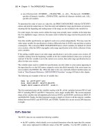
Output 8.4.1 Autocorrelation-Corrected Regression Results
Simulated Time Series with Roots:
(X-1.25)(X
**
4-1.25)
With 15% Missing Values
The AUTOREG Procedure
Dependent Variable y
Ordinary Least Squares Estimates
SSE 182.972379 DFE 40
MSE 4.57431 Root MSE 2.13876
SBC 181.39282 AIC 179.679248
MAE 1.80469152 AICC 179.781813
MAPE 270.104379 HQC 180.303237
Durbin-Watson 1.3962 Regress R-Square 0.0000
Total R-Square 0.0000
Parameter Estimates
Standard Approx
Variable DF Estimate Error t Value Pr > |t|
Intercept 1 -2.2387 0.3340 -6.70 <.0001
Estimates of Autocorrelations
Lag Covariance Correlation -1 9 8 7 6 5 4 3 2 1 0 1 2 3 4 5 6 7 8 9 1

0 4.4627 1.000000 | |
********************
|
1 1.4241 0.319109 | |
******
|
2 1.6505 0.369829 | |
*******
|
3 0.6808 0.152551 | |
***
|
4 2.9167 0.653556 | |
*************
|
5 -0.3816 -0.085519 |
**
| |
Partial
Autocorrelations
1 0.319109
4 0.619288
5 -0.821179
Example 8.4: Missing Values ✦ 431
Output 8.4.1 continued
Preliminary MSE 0.7609
Estimates of Autoregressive Parameters
Standard
Lag Coefficient Error t Value
1 -0.733182 0.089966 -8.15

4 -0.803754 0.071849 -11.19
5 0.821179 0.093818 8.75
Expected
Autocorrelations
Lag Autocorr
0 1.0000
1 0.4204
2 0.2480
3 0.3160
4 0.6903
5 0.0228
Algorithm converged.
Maximum Likelihood Estimates
SSE 48.4396756 DFE 37
MSE 1.30918 Root MSE 1.14419
SBC 146.879013 AIC 140.024725
MAE 0.88786192 AICC 141.135836
MAPE 141.377721 HQC 142.520679
Durbin-Watson 2.9457 Regress R-Square 0.0000
Total R-Square 0.7353
Parameter Estimates
Standard Approx
Variable DF Estimate Error t Value Pr > |t|
Intercept 1 -2.2370 0.5239 -4.27 0.0001
AR1 1 -0.6201 0.1129 -5.49 <.0001
AR4 1 -0.7237 0.0914 -7.92 <.0001
AR5 1 0.6550 0.1202 5.45 <.0001