SAS/ETS 9.22 User''''s Guide 21 doc

192
Chapter 7
The ARIMA Procedure
Contents
Overview: ARIMA Procedure . . . . . . . . . . . . . . . . . . . . . . . . . . . . 194
Getting Started: ARIMA Procedure . . . . . . . . . . . . . . . . . . . . . . . . . 195
The Three Stages of ARIMA Modeling . . . . . . . . . . . . . . . . . . . . 195
Identification Stage . . . . . . . . . . . . . . . . . . . . . . . . . . . . . . . 196
Estimation and Diagnostic Checking Stage . . . . . . . . . . . . . . . . . . . 201
Forecasting Stage . . . . . . . . . . . . . . . . . . . . . . . . . . . . . . . . 207
Using ARIMA Procedure Statements . . . . . . . . . . . . . . . . . . . . . 209
General Notation for ARIMA Models . . . . . . . . . . . . . . . . . . . . . 210
Stationarity . . . . . . . . . . . . . . . . . . . . . . . . . . . . . . . . . . . 213
Differencing . . . . . . . . . . . . . . . . . . . . . . . . . . . . . . . . . . 213
Subset, Seasonal, and Factored ARMA Models . . . . . . . . . . . . . . . . 215
Input Variables and Regression with ARMA Errors . . . . . . . . . . . . . . 216
Intervention Models and Interrupted Time Series . . . . . . . . . . . . . . . 219
Rational Transfer Functions and Distributed Lag Models . . . . . . . . . . . . 221
Forecasting with Input Variables . . . . . . . . . . . . . . . . . . . . . . . . 223
Data Requirements . . . . . . . . . . . . . . . . . . . . . . . . . . . . . . . 224
Syntax: ARIMA Procedure . . . . . . . . . . . . . . . . . . . . . . . . . . . . . . 224
Functional Summary . . . . . . . . . . . . . . . . . . . . . . . . . . . . . . 225
PROC ARIMA Statement . . . . . . . . . . . . . . . . . . . . . . . . . . . . 227
BY Statement . . . . . . . . . . . . . . . . . . . . . . . . . . . . . . . . . . 231
IDENTIFY Statement . . . . . . . . . . . . . . . . . . . . . . . . . . . . . . 231
ESTIMATE Statement . . . . . . . . . . . . . . . . . . . . . . . . . . . . . 235
OUTLIER Statement . . . . . . . . . . . . . . . . . . . . . . . . . . . . . . 240
FORECAST Statement . . . . . . . . . . . . . . . . . . . . . . . . . . . . . 241
Details: ARIMA Procedure . . . . . . . . . . . . . . . . . . . . . . . . . . . . . . 243
The Inverse Autocorrelation Function . . . . . . . . . . . . . . . . . . . . . 243
The Partial Autocorrelation Function . . . . . . . . . . . . . . . . . . . . . 244

The Cross-Correlation Function . . . . . . . . . . . . . . . . . . . . . . . . 244
The ESACF Method . . . . . . . . . . . . . . . . . . . . . . . . . . . . . . 245
The MINIC Method . . . . . . . . . . . . . . . . . . . . . . . . . . . . . . 246
The SCAN Method . . . . . . . . . . . . . . . . . . . . . . . . . . . . . . . 248
Stationarity Tests . . . . . . . . . . . . . . . . . . . . . . . . . . . . . . . . 250
Prewhitening . . . . . . . . . . . . . . . . . . . . . . . . . . . . . . . . . . 250
Identifying Transfer Function Models . . . . . . . . . . . . . . . . . . . . . . 251
194 ✦ Chapter 7: The ARIMA Procedure
Missing Values and Autocorrelations . . . . . . . . . . . . . . . . . . . . . . 251
Estimation Details . . . . . . . . . . . . . . . . . . . . . . . . . . . . . . . 252
Specifying Inputs and Transfer Functions . . . . . . . . . . . . . . . . . . . 256
Initial Values . . . . . . . . . . . . . . . . . . . . . . . . . . . . . . . . . . 258
Stationarity and Invertibility . . . . . . . . . . . . . . . . . . . . . . . . . . 259
Naming of Model Parameters . . . . . . . . . . . . . . . . . . . . . . . . . 259
Missing Values and Estimation and Forecasting . . . . . . . . . . . . . . . . 260
Forecasting Details . . . . . . . . . . . . . . . . . . . . . . . . . . . . . . . 260
Forecasting Log Transformed Data . . . . . . . . . . . . . . . . . . . . . . 262
Specifying Series Periodicity . . . . . . . . . . . . . . . . . . . . . . . . . 263
Detecting Outliers . . . . . . . . . . . . . . . . . . . . . . . . . . . . . . . 263
OUT= Data Set . . . . . . . . . . . . . . . . . . . . . . . . . . . . . . . . . 265
OUTCOV= Data Set . . . . . . . . . . . . . . . . . . . . . . . . . . . . . . . 267
OUTEST= Data Set . . . . . . . . . . . . . . . . . . . . . . . . . . . . . . . 267
OUTMODEL= SAS Data Set . . . . . . . . . . . . . . . . . . . . . . . . . 270
OUTSTAT= Data Set . . . . . . . . . . . . . . . . . . . . . . . . . . . . . . 272
Printed Output . . . . . . . . . . . . . . . . . . . . . . . . . . . . . . . . . 273
ODS Table Names . . . . . . . . . . . . . . . . . . . . . . . . . . . . . . . 275
Statistical Graphics . . . . . . . . . . . . . . . . . . . . . . . . . . . . . . . . 277
Examples: ARIMA Procedure . . . . . . . . . . . . . . . . . . . . . . . . . . . . 280
Example 7.1: Simulated IMA Model . . . . . . . . . . . . . . . . . . . . . 280
Example 7.2: Seasonal Model for the Airline Series . . . . . . . . . . . . . 285

Example 7.3: Model for Series J Data from Box and Jenkins . . . . . . . . 292
Example 7.4: An Intervention Model for Ozone Data . . . . . . . . . . . . . 301
Example 7.5: Using Diagnostics to Identify ARIMA Models . . . . . . . . 303
Example 7.6: Detection of Level Changes in the Nile River Data . . . . . . 308
Example 7.7: Iterative Outlier Detection . . . . . . . . . . . . . . . . . . . 310
References . . . . . . . . . . . . . . . . . . . . . . . . . . . . . . . . . . . . . . 313
Overview: ARIMA Procedure
The ARIMA procedure analyzes and forecasts equally spaced univariate time series data, transfer
function data, and intervention data by using the autoregressive integrated moving-average (ARIMA)
or autoregressive moving-average (ARMA) model. An ARIMA model predicts a value in a re-
sponse time series as a linear combination of its own past values, past errors (also called shocks or
innovations), and current and past values of other time series.
The ARIMA approach was first popularized by Box and Jenkins, and ARIMA models are often
referred to as Box-Jenkins models. The general transfer function model employed by the ARIMA
procedure was discussed by Box and Tiao (1975). When an ARIMA model includes other time
series as input variables, the model is sometimes referred to as an ARIMAX model. Pankratz (1991)
refers to the ARIMAX model as dynamic regression.
Getting Started: ARIMA Procedure ✦ 195
The ARIMA procedure provides a comprehensive set of tools for univariate time series model
identification, parameter estimation, and forecasting, and it offers great flexibility in the kinds of
ARIMA or ARIMAX models that can be analyzed. The ARIMA procedure supports seasonal, subset,
and factored ARIMA models; intervention or interrupted time series models; multiple regression
analysis with ARMA errors; and rational transfer function models of any complexity.
The design of PROC ARIMA closely follows the Box-Jenkins strategy for time series modeling
with features for the identification, estimation and diagnostic checking, and forecasting steps of the
Box-Jenkins method.
Before you use PROC ARIMA, you should be familiar with Box-Jenkins methods, and you should
exercise care and judgment when you use the ARIMA procedure. The ARIMA class of time series
models is complex and powerful, and some degree of expertise is needed to use them correctly.
Getting Started: ARIMA Procedure

This section outlines the use of the ARIMA procedure and gives a cursory description of the ARIMA
modeling process for readers who are less familiar with these methods.
The Three Stages of ARIMA Modeling
The analysis performed by PROC ARIMA is divided into three stages, corresponding to the stages
described by Box and Jenkins (1976).
1.
In the identification stage, you use the IDENTIFY statement to specify the response series
and identify candidate ARIMA models for it. The IDENTIFY statement reads time series that
are to be used in later statements, possibly differencing them, and computes autocorrelations,
inverse autocorrelations, partial autocorrelations, and cross-correlations. Stationarity tests
can be performed to determine if differencing is necessary. The analysis of the IDENTIFY
statement output usually suggests one or more ARIMA models that could be fit. Options
enable you to test for stationarity and tentative ARMA order identification.
2.
In the estimation and diagnostic checking stage, you use the ESTIMATE statement to specify
the ARIMA model to fit to the variable specified in the previous IDENTIFY statement and to
estimate the parameters of that model. The ESTIMATE statement also produces diagnostic
statistics to help you judge the adequacy of the model.
Significance tests for parameter estimates indicate whether some terms in the model might be
unnecessary. Goodness-of-fit statistics aid in comparing this model to others. Tests for white
noise residuals indicate whether the residual series contains additional information that might
be used by a more complex model. The OUTLIER statement provides another useful tool to
check whether the currently estimated model accounts for all the variation in the series. If the
diagnostic tests indicate problems with the model, you try another model and then repeat the
estimation and diagnostic checking stage.
196 ✦ Chapter 7: The ARIMA Procedure
3.
In the forecasting stage, you use the FORECAST statement to forecast future values of the
time series and to generate confidence intervals for these forecasts from the ARIMA model
produced by the preceding ESTIMATE statement.

These three steps are explained further and illustrated through an extended example in the following
sections.
Identification Stage
Suppose you have a variable called SALES that you want to forecast. The following example
illustrates ARIMA modeling and forecasting by using a simulated data set TEST that contains a
time series SALES generated by an ARIMA(1,1,1) model. The output produced by this example is
explained in the following sections. The simulated SALES series is shown in Figure 7.1.
ods graphics on;
proc sgplot data=test;
scatter y=sales x=date;
run;
Figure 7.1 Simulated ARIMA(1,1,1) Series SALES
Identification Stage ✦ 197
Using the IDENTIFY Statement
You first specify the input data set in the PROC ARIMA statement. Then, you use an IDENTIFY
statement to read in the SALES series and analyze its correlation properties. You do this by using the
following statements:
proc arima data=test ;
identify var=sales nlag=24;
run;
Descriptive Statistics
The IDENTIFY statement first prints descriptive statistics for the SALES series. This part of the
IDENTIFY statement output is shown in Figure 7.2.
Figure 7.2 IDENTIFY Statement Descriptive Statistics Output
The ARIMA Procedure
Name of Variable = sales
Mean of Working Series 137.3662
Standard Deviation 17.36385
Number of Observations 100
Autocorrelation Function Plots

The IDENTIFY statement next produces a panel of plots used for its autocorrelation and trend
analysis. The panel contains the following plots:
 the time series plot of the series
 the sample autocorrelation function plot (ACF)
 the sample inverse autocorrelation function plot (IACF)
 the sample partial autocorrelation function plot (PACF)
This correlation analysis panel is shown in Figure 7.3.
198 ✦ Chapter 7: The ARIMA Procedure
Figure 7.3 Correlation Analysis of SALES
These autocorrelation function plots show the degree of correlation with past values of the series as a
function of the number of periods in the past (that is, the lag) at which the correlation is computed.
The NLAG= option controls the number of lags for which the autocorrelations are shown. By default,
the autocorrelation functions are plotted to lag 24.
Most books on time series analysis explain how to interpret the autocorrelation and the partial
autocorrelation plots. See the section “The Inverse Autocorrelation Function” on page 243 for a
discussion of the inverse autocorrelation plots.
By examining these plots, you can judge whether the series is stationary or nonstationary. In
this case, a visual inspection of the autocorrelation function plot indicates that the SALES series
is nonstationary, since the ACF decays very slowly. For more formal stationarity tests, use the
STATIONARITY= option. (See the section “Stationarity” on page 213.)
White Noise Test
The last part of the default IDENTIFY statement output is the check for white noise. This is an
approximate statistical test of the hypothesis that none of the autocorrelations of the series up to a
Identification Stage ✦ 199
given lag are significantly different from 0. If this is true for all lags, then there is no information in
the series to model, and no ARIMA model is needed for the series.
The autocorrelations are checked in groups of six, and the number of lags checked depends on the
NLAG= option. The check for white noise output is shown in Figure 7.4.
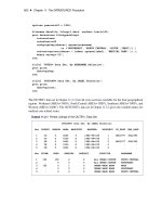
Figure 7.4 IDENTIFY Statement Check for White Noise
Autocorrelation Check for White Noise

To Chi- Pr >
Lag Square DF ChiSq Autocorrelations
6 426.44 6 <.0001 0.957 0.907 0.852 0.791 0.726 0.659
12 547.82 12 <.0001 0.588 0.514 0.440 0.370 0.303 0.238
18 554.70 18 <.0001 0.174 0.112 0.052 -0.004 -0.054 -0.098
24 585.73 24 <.0001 -0.135 -0.167 -0.192 -0.211 -0.227 -0.240
In this case, the white noise hypothesis is rejected very strongly, which is expected since the series is
nonstationary. The p-value for the test of the first six autocorrelations is printed as <0.0001, which
means the p-value is less than 0.0001.
Identification of the Differenced Series
Since the series is nonstationary, the next step is to transform it to a stationary series by differencing.
That is, instead of modeling the SALES series itself, you model the change in SALES from one period
to the next. To difference the SALES series, use another IDENTIFY statement and specify that the
first difference of SALES be analyzed, as shown in the following statements:
proc arima data=test;
identify var=sales(1);
run;
The second IDENTIFY statement produces the same information as the first, but for the change in
SALES from one period to the next rather than for the total SALES in each period. The summary
statistics output from this IDENTIFY statement is shown in Figure 7.5. Note that the period of
differencing is given as 1, and one observation was lost through the differencing operation.
Figure 7.5 IDENTIFY Statement Output for Differenced Series
The ARIMA Procedure
Name of Variable = sales
Period(s) of Differencing 1
Mean of Working Series 0.660589
Standard Deviation 2.011543
Number of Observations 99
Observation(s) eliminated by differencing 1
200 ✦ Chapter 7: The ARIMA Procedure

The autocorrelation plots for the differenced series are shown in Figure 7.6.
Figure 7.6 Correlation Analysis of the Change in SALES
The autocorrelations decrease rapidly in this plot, indicating that the change in SALES is a stationary
time series.
The next step in the Box-Jenkins methodology is to examine the patterns in the autocorrelation plot
to choose candidate ARMA models to the series. The partial and inverse autocorrelation function
plots are also useful aids in identifying appropriate ARMA models for the series.
In the usual Box-Jenkins approach to ARIMA modeling, the sample autocorrelation function, inverse
autocorrelation function, and partial autocorrelation function are compared with the theoretical
correlation functions expected from different kinds of ARMA models. This matching of theoretical
autocorrelation functions of different ARMA models to the sample autocorrelation functions com-
puted from the response series is the heart of the identification stage of Box-Jenkins modeling. Most
textbooks on time series analysis, such as Pankratz (1983), discuss the theoretical autocorrelation
functions for different kinds of ARMA models.
Since the input data are only a limited sample of the series, the sample autocorrelation functions
computed from the input series only approximate the true autocorrelation function of the process
that generates the series. This means that the sample autocorrelation functions do not exactly match
the theoretical autocorrelation functions for any ARMA model and can have a pattern similar to that
Estimation and Diagnostic Checking Stage ✦ 201
of several different ARMA models. If the series is white noise (a purely random process), then there
is no need to fit a model. The check for white noise, shown in Figure 7.7, indicates that the change in
SALES is highly autocorrelated. Thus, an autocorrelation model, for example an AR(1) model, might
be a good candidate model to fit to this process.
Figure 7.7 IDENTIFY Statement Check for White Noise
Autocorrelation Check for White Noise
To Chi- Pr >
Lag Square DF ChiSq Autocorrelations
6 154.44 6 <.0001 0.828 0.591 0.454 0.369 0.281 0.198
12 173.66 12 <.0001 0.151 0.081 -0.039 -0.141 -0.210 -0.274
18 209.64 18 <.0001 -0.305 -0.271 -0.218 -0.183 -0.174 -0.161

24 218.04 24 <.0001 -0.144 -0.141 -0.125 -0.085 -0.040 -0.032
Estimation and Diagnostic Checking Stage
The autocorrelation plots for this series, as shown in the previous section, suggest an AR(1) model
for the change in SALES. You should check the diagnostic statistics to see if the AR(1) model is
adequate. Other candidate models include an MA(1) model and low-order mixed ARMA models. In
this example, the AR(1) model is tried first.
Estimating an AR(1) Model
The following statements fit an AR(1) model (an autoregressive model of order 1), which predicts
the change in SALES as an average change, plus some fraction of the previous change, plus a random
error. To estimate an AR model, you specify the order of the autoregressive model with the P= option
in an ESTIMATE statement:
estimate p=1;
run;
The ESTIMATE statement fits the model to the data and prints parameter estimates and various
diagnostic statistics that indicate how well the model fits the data. The first part of the ESTIMATE
statement output, the table of parameter estimates, is shown in Figure 7.8.