SAS/ETS 9.22 User''''s Guide 27 doc

252 ✦ Chapter 7: The ARIMA Procedure
Estimation Details
The ARIMA procedure primarily uses the computational methods outlined by Box and Jenkins.
Marquardt’s method is used for the nonlinear least squares iterations. Numerical approximations
of the derivatives of the sum-of-squares function are taken by using a fixed delta (controlled by the
DELTA= option).
The methods do not always converge successfully for a given set of data, particularly if the starting
values for the parameters are not close to the least squares estimates.
Back-Forecasting
The unconditional sum of squares is computed exactly; thus, back-forecasting is not performed.
Early versions of SAS/ETS software used the back-forecasting approximation and allowed a positive
value of the BACKLIM= option to control the extent of the back-forecasting. In the current version,
requesting a positive number of back-forecasting steps with the BACKLIM= option has no effect.
Preliminary Estimation
If an autoregressive or moving-average operator is specified with no missing lags, preliminary
estimates of the parameters are computed by using the autocorrelations computed in the IDEN-
TIFY stage. Otherwise, the preliminary estimates are arbitrarily set to values that produce stable
polynomials.
When preliminary estimation is not performed by PROC ARIMA, then initial values of the coef-
ficients for any given autoregressive or moving-average factor are set to 0.1 if the degree of the
polynomial associated with the factor is 9 or less. Otherwise, the coefficients are determined by
expanding the polynomial (1 0:1B) to an appropriate power by using a recursive algorithm.
These preliminary estimates are the starting values in an iterative algorithm to compute estimates of
the parameters.
Estimation Methods
Maximum Likelihood
The METHOD= ML option produces maximum likelihood estimates. The likelihood function is
maximized via nonlinear least squares using Marquardt’s method. Maximum likelihood estimates
are more expensive to compute than the conditional least squares estimates; however, they may be
preferable in some cases (Ansley and Newbold 1980; Davidson 1981).
The maximum likelihood estimates are computed as follows. Let the univariate ARMA model be

.B/.W
t
 
t
/ D Â.B/a
t
where a
t
is an independent sequence of normally distributed innovations with mean 0 and variance

2
. Here

t
is the mean parameter

plus the transfer function inputs. The log-likelihood function
Estimation Details ✦ 253
can be written as follows:

1
2
2
x
0

1
x 
1
2

ln.jj/ 
n
2
ln.
2
/
In this equation, n is the number of observations,

2

is the variance of
x
as a function of the

and
Â
parameters, and
jj
denotes the determinant. The vector
x
is the time series
W
t
minus the
structural part of the model 
t
, written as a column vector, as follows:
x D
2
6

6
6
4
W
1
W
2
:
:
:
W
n
3
7
7
7
5

2
6
6
6
4

1

2
:
:
:


n
3
7
7
7
5
The maximum likelihood estimate (MLE) of 
2
is
s
2
D
1
n
x
0

1
x
Note that the default estimator of the variance divides by
n  r
, where r is the number of parameters
in the model, instead of by n. Specifying the NODF option causes a divisor of n to be used.
The log-likelihood concentrated with respect to 
2
can be taken up to additive constants as

n
2

ln.x
0

1
x/ 
1
2
ln.jj/
Let
H
be the lower triangular matrix with positive elements on the diagonal such that
HH
0
D 
. Let
e be the vector H
1
x. The concentrated log-likelihood with respect to 
2
can now be written as

n
2
ln.e
0
e/  ln.jHj/
or

n
2

ln.jHj
1=n
e
0
ejHj
1=n
/
The MLE is produced by using a Marquardt algorithm to minimize the following sum of squares:
jHj
1=n
e
0
ejHj
1=n
The subsequent analysis of the residuals is done by using e as the vector of residuals.
Unconditional Least Squares
The METHOD=ULS option produces unconditional least squares estimates. The ULS method is also
referred to as the exact least squares (ELS) method. For METHOD=ULS, the estimates minimize
n
X
tD1
Qa
2
t
D
n
X
tD1
.x
t

 C
t
V
1
t
.x
1
; ; x
t1
/
0
/
2
where
C
t
is the covariance matrix of
x
t
and
.x
1
; ; x
t1
/
, and
V
t
is the variance matrix of
.x

1
; ; x
t1
/
. In fact,
P
n
tD1
Qa
2
t
is the same as
x
0

1
x
, and hence
e
0
e
. Therefore, the uncon-
ditional least squares estimates are obtained by minimizing the sum of squared residuals rather than
using the log-likelihood as the criterion function.
254 ✦ Chapter 7: The ARIMA Procedure
Conditional Least Squares
The METHOD=CLS option produces conditional least squares estimates. The CLS estimates are
conditional on the assumption that the past unobserved errors are equal to 0. The series
x
t

can be
represented in terms of the previous observations, as follows:
x
t
D a
t
C
1
X
iD1

i
x
ti
The  weights are computed from the ratio of the  and  polynomials, as follows:
.B/
Â.B/
D 1 
1
X
iD1

i
B
i
The CLS method produces estimates minimizing
n
X
tD1
Oa

2
t
D
n
X
tD1
.x
t

1
X
iD1
O
i
x
ti
/
2
where the unobserved past values of
x
t
are set to 0 and
O
i
are computed from the estimates of

and
 at each iteration.
For METHOD=ULS and METHOD=ML, initial estimates are computed using the METHOD=CLS
algorithm.

Start-up for Transfer Functions
When computing the noise series for transfer function and intervention models, the start-up for
the transferred variable is done by assuming that past values of the input series are equal to the
first value of the series. The estimates are then obtained by applying least squares or maximum
likelihood to the noise series. Thus, for transfer function models, the ML option does not generate the
full (multivariate ARMA) maximum likelihood estimates, but it uses only the univariate likelihood
function applied to the noise series.
Because PROC ARIMA uses all of the available data for the input series to generate the noise series,
other start-up options for the transferred series can be implemented by prefixing an observation to
the beginning of the real data. For example, if you fit a transfer function model to the variable Y
with the single input X, then you can employ a start-up using 0 for the past values by prefixing to the
actual data an observation with a missing value for Y and a value of 0 for X.
Information Criteria
PROC ARIMA computes and prints two information criteria, Akaike’s information criterion (AIC)
(Akaike 1974; Harvey 1981) and Schwarz’s Bayesian criterion (SBC) (Schwarz 1978). The AIC
and SBC are used to compare competing models fit to the same series. The model with the smaller
information criteria is said to fit the data better. The AIC is computed as
2ln.L/ C 2k
Estimation Details ✦ 255
where L is the likelihood function and k is the number of free parameters. The SBC is computed as
2ln.L/ C ln.n/k
where n is the number of residuals that can be computed for the time series. Sometimes Schwarz’s
Bayesian criterion is called the Bayesian information criterion (BIC).
If METHOD=CLS is used to do the estimation, an approximation value of L is used, where L is
based on the conditional sum of squares instead of the exact sum of squares, and a Jacobian factor is
left out.
Tests of Residuals
A table of test statistics for the hypothesis that the model residuals are white noise is printed as
part of the ESTIMATE statement output. The chi-square statistics used in the test for lack of fit are
computed using the Ljung-Box formula


2
m
D n.n C2/
m
X
kD1
r
2
k
.n  k/
where
r
k
D
P
nk
tD1
a
t
a
tCk
P
n
tD1
a
2
t
and a
t

is the residual series.
This formula has been suggested by Ljung and Box (1978) as yielding a better fit to the asymptotic
chi-square distribution than the Box-Pierce Q statistic. Some simulation studies of the finite sample
properties of this statistic are given by Davies, Triggs, and Newbold (1977) and by Ljung and Box
(1978). When the time series has missing values, Stoffer and Toloi (1992) suggest a modification of
this test statistic that has improved distributional properties over the standard Ljung-Box formula
given above. When the series contains missing values, this modified test statistic is used by default.
Each chi-square statistic is computed for all lags up to the indicated lag value and is not independent of
the preceding chi-square values. The null hypotheses tested is that the current set of autocorrelations
is white noise.
t-values
The t values reported in the table of parameter estimates are approximations whose accuracy depends
on the validity of the model, the nature of the model, and the length of the observed series. When the
length of the observed series is short and the number of estimated parameters is large with respect
to the series length, the t approximation is usually poor. Probability values that correspond to a t
distribution should be interpreted carefully because they may be misleading.
256 ✦ Chapter 7: The ARIMA Procedure
Cautions during Estimation
The ARIMA procedure uses a general nonlinear least squares estimation method that can yield
problematic results if your data do not fit the model. Output should be examined carefully. The GRID
option can be used to ensure the validity and quality of the results. Problems you might encounter
include the following:

Preliminary moving-average estimates might not converge. If this occurs, preliminary estimates
are derived as described previously in “Preliminary Estimation” on page 252. You can supply
your own preliminary estimates with the ESTIMATE statement options.

The estimates can lead to an unstable time series process, which can cause extreme forecast
values or overflows in the forecast.


The Jacobian matrix of partial derivatives might be singular; usually, this happens because not
all the parameters are identifiable. Removing some of the parameters or using a longer time
series might help.

The iterative process might not converge. PROC ARIMA’s estimation method stops after n
iterations, where n is the value of the MAXITER= option. If an iteration does not improve
the SSE, the Marquardt parameter is increased by a factor of ten until parameters that have a
smaller SSE are obtained or until the limit value of the Marquardt parameter is exceeded.

For METHOD=CLS, the estimates might converge but not to least squares estimates. The
estimates might converge to a local minimum, the numerical calculations might be distorted
by data whose sum-of-squares surface is not smooth, or the minimum might lie outside the
region of invertibility or stationarity.

If the data are differenced and a moving-average model is fit, the parameter estimates might
try to converge exactly on the invertibility boundary. In this case, the standard error estimates
that are based on derivatives might be inaccurate.
Specifying Inputs and Transfer Functions
Input variables and transfer functions for them can be specified using the INPUT= option in the ESTI-
MATE statement. The variables used in the INPUT= option must be included in the CROSSCORR=
list in the previous IDENTIFY statement. If any differencing is specified in the CROSSCORR= list,
then the differenced variable is used as the input to the transfer function.
General Syntax of the INPUT= Option
The general syntax of the INPUT= option is
ESTIMATE . . . INPUT=( transfer-function variable . . . )
The transfer function for an input variable is optional. The name of a variable by itself can be used to
specify a pure regression term for the variable.
Specifying Inputs and Transfer Functions ✦ 257
If specified, the syntax of the transfer function is
S $ .L

1;1
; L
1;2
; : : :/.L
2;1
; : : :/: : :=.L
i;1
; L
i;2
; : : :/.L
iC1;1
; : : :/: : :
S is the number of periods of time delay (lag) for this input series. Each term in parentheses specifies
a polynomial factor with parameters at the lags specified by the
L
i;j
values. The terms before the
slash (/) are numerator factors. The terms after the slash (/) are denominator factors. All three parts
are optional.
Commas can optionally be used between input specifications to make the INPUT= option more
readable. The $ sign after the shift is also optional.
Except for the first numerator factor, each of the terms
L
i;1
; L
i;2
; : : :; L
i;k
indicates a factor of the
form

.1  !
i;1
B
L
i;1
 !
i;2
B
L
i;2
 : : :  !
i;k
B
L
i;k
/
The form of the first numerator factor depends on the ALTPARM option. By default, the constant 1
in the first numerator factor is replaced with a free parameter !
0
.
Alternative Model Parameterization
When the ALTPARM option is specified, the
!
0
parameter is factored out so that it multiplies the
entire transfer function, and the first numerator factor has the same form as the other factors.
The ALTPARM option does not materially affect the results; it just presents the results differently.
Some people prefer to see the model written one way, while others prefer the alternative representation.
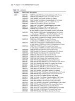
Table 7.9 illustrates the effect of the ALTPARM option.
Table 7.9 The ALTPARM Option

INPUT= Option ALTPARM Model
INPUT=((1 2)(12)/(1)X); No .!
0
 !
1
B  !
2
B
2
/.1  !
3
B
12
/=.1  ı
1
B/X
t
Yes !
0
.1  !
1
B  !
2
B
2
/.1  !
3
B
12
/=.1  ı

1
B/X
t
Differencing and Input Variables
If you difference the response series and use input variables, take care that the differencing operations
do not change the meaning of the model. For example, if you want to fit the model
Y
t
D
!
0
.1  ı
1
B/
X
t
C
.1  Â
1
B/
.1  B/.1 B
12
/
a
t
then the IDENTIFY statement must read
identify var=y(1,12) crosscorr=x(1,12);
estimate q=1 input=(/(1)x) noconstant;
258 ✦ Chapter 7: The ARIMA Procedure
If instead you specify the differencing as

identify var=y(1,12) crosscorr=x;
estimate q=1 input=(/(1)x) noconstant;
then the model being requested is
Y
t
D
!
0
.1  ı
1
B/.1 B/.1  B
12
/
X
t
C
.1  Â
1
B/
.1  B/.1 B
12
/
a
t
which is a very different model.
The point to remember is that a differencing operation requested for the response variable specified
by the VAR= option is applied only to that variable and not to the noise term of the model.
Initial Values
The syntax for giving initial values to transfer function parameters in the INITVAL= option parallels
the syntax of the INPUT= option. For each transfer function in the INPUT= option, the INITVAL=

option should give an initialization specification followed by the input series name. The initialization
specification for each transfer function has the form
C $ .V
1;1
; V
1;2
; : : :/.V
2;1
; : : :/: : :=.V
i;1
; : : :/: : :
where C is the lag 0 term in the first numerator factor of the transfer function (or the overall scale
factor if the ALTPARM option is specified) and
V
i;j
is the coefficient of the
L
i;j
element in the
transfer function.
To illustrate, suppose you want to fit the model
Y
t
D  C
.!
0
 !
1
B  !
2

B
2
/
.1  ı
1
B  ı
2
B
2
 ı
3
B
3
/
X
t3
C
1
.1  
1
B  
2
B
3
/
a
t
and start the estimation process with the initial values =10, !
0
=1, !

1
=0.5, !
2
=0.03, ı
1
=0.8,
ı
2
=–0.1,
ı
3
=0.002,

1
=0.1,

2
=0.01. (These are arbitrary values for illustration only.) You would
use the following statements:
identify var=y crosscorr=x;
estimate p=(1,3) input=(3$(1,2)/(1,2,3)x)
mu=10 ar=.1 .01
initval=(1$(.5,.03)/(.8, 1,.002)x);
Note that the lags specified for a particular factor are sorted, so initial values should be given in
sorted order. For example, if the P= option had been entered as P=(3,1) instead of P=(1,3), the model
would be the same and so would the AR= option. Sorting is done within all factors, including transfer
function factors, so initial values should always be given in order of increasing lags.
Stationarity and Invertibility ✦ 259
Here is another illustration, showing initialization for a factored model with multiple inputs. The
model is

Y
t
D  C
!
1;0
.1  ı
1;1
B/
W
t
C .!
2;0
 !
2;1
B/X
t3
C
1
.1  
1
B/.1 
2
B
6
 
3
B
12
/
a

t
and the initial values are

=10,
!
1;0
=5,
ı
1;1
=0.8,
!
2;0
=1,
!
2;1
=0.5,

1
=0.1,

2
=0.05, and

3
=0.01.
You would use the following statements:
identify var=y crosscorr=(w x);
estimate p=(1)(6,12) input=(/(1)w, 3$(1)x)
mu=10 ar=.1 .05 .01
initval=(5$/(.8)w 1$(.5)x);

Stationarity and Invertibility
By default, PROC ARIMA requires that the parameter estimates for the AR and MA parts of the
model always remain in the stationary and invertible regions, respectively. The NOSTABLE option
removes this restriction and for high-order models can save some computer time. Note that using the
NOSTABLE option does not necessarily result in an unstable model being fit, since the estimates can
leave the stable region for some iterations but still ultimately converge to stable values. Similarly,
by default, the parameter estimates for the denominator polynomial of the transfer function part of
the model are also restricted to be stable. The NOTFSTABLE option can be used to remove this
restriction.
Naming of Model Parameters
In the table of parameter estimates produced by the ESTIMATE statement, model parameters are
referred to by using the naming convention described in this section.
The parameters in the noise part of the model are named as ARi,j or MAi,j, where AR refers to
autoregressive parameters and MA to moving-average parameters. The subscript i refers to the
particular polynomial factor, and the subscript j refers to the jth term within the ith factor. These
terms are sorted in order of increasing lag within factors, so the subscript j refers to the jth term after
sorting.
When inputs are used in the model, the parameters of each transfer function are named NUMi,j and
DENi,j. The jth term in the ith factor of a numerator polynomial is named NUMi,j. The jth term in
the ith factor of a denominator polynomial is named DENi,j.
This naming process is repeated for each input variable, so if there are multiple inputs, parameters in
transfer functions for different input series have the same name. The table of parameter estimates
260 ✦ Chapter 7: The ARIMA Procedure
shows in the “Variable” column the input with which each parameter is associated. The parameter
name shown in the “Parameter” column and the input variable name shown in the “Variable” column
must be combined to fully identify transfer function parameters.
The lag 0 parameter in the first numerator factor for the first input variable is named NUM1. For
subsequent input variables, the lag 0 parameter in the first numerator factor is named NUMk, where
k is the position of the input variable in the INPUT= option list. If the ALTPARM option is specified,
the NUMk parameter is replaced by an overall scale parameter named SCALEk.

For the mean and noise process parameters, the response series name is shown in the “Variable”
column. The lag and shift for each parameter are also shown in the table of parameter estimates
when inputs are used.
Missing Values and Estimation and Forecasting
Estimation and forecasting are carried out in the presence of missing values by forecasting the
missing values with the current set of parameter estimates. The maximum likelihood algorithm
employed was suggested by Jones (1980) and is used for both unconditional least squares (ULS) and
maximum likelihood (ML) estimation.
The CLS algorithm simply fills in missing values with infinite memory forecast values, computed by
forecasting ahead from the nonmissing past values as far as required by the structure of the missing
values. These artificial values are then employed in the nonmissing value CLS algorithm. Artificial
values are updated at each iteration along with parameter estimates.
For models with input variables, embedded missing values (that is, missing values other than at
the beginning or end of the series) are not generally supported. Embedded missing values in input
variables are supported for the special case of a multiple regression model that has ARIMA errors.
A multiple regression model is specified by an INPUT= option that simply lists the input variables
(possibly with lag shifts) without any numerator or denominator transfer function factors. One-step-
ahead forecasts are not available for the response variable when one or more of the input variables
have missing values.
When embedded missing values are present for a model with complex transfer functions, PROC
ARIMA uses the first continuous nonmissing piece of each series to do the analysis. That is, PROC
ARIMA skips observations at the beginning of each series until it encounters a nonmissing value and
then uses the data from there until it encounters another missing value or until the end of the data is
reached. This makes the current version of PROC ARIMA compatible with earlier releases that did
not allow embedded missing values.
Forecasting Details
If the model has input variables, a forecast beyond the end of the data for the input variables is
possible only if univariate ARIMA models have previously been fit to the input variables or future
values for the input variables are included in the DATA= data set.
Forecasting Details ✦ 261

If input variables are used, the forecast standard errors and confidence limits of the response depend
on the estimated forecast error variance of the predicted inputs. If several input series are used, the
forecast errors for the inputs should be independent; otherwise, the standard errors and confidence
limits for the response series will not be accurate. If future values for the input variables are included
in the DATA= data set, the standard errors of the forecasts will be underestimated since these values
are assumed to be known with certainty.
The forecasts are generated using forecasting equations consistent with the method used to estimate
the model parameters. Thus, the estimation method specified in the ESTIMATE statement also
controls the way forecasts are produced by the FORECAST statement. If METHOD=CLS is used,
the forecasts are infinite memory forecasts, also called conditional forecasts. If METHOD=ULS or
METHOD=ML, the forecasts are finite memory forecasts, also called unconditional forecasts. A
complete description of the steps to produce the series forecasts and their standard errors by using
either of these methods is quite involved, and only a brief explanation of the algorithm is given in the
next two sections. Additional details about the finite and infinite memory forecasts can be found in
Brockwell and Davis (1991). The prediction of stationary ARMA processes is explained in Chapter
5, and the prediction of nonstationary ARMA processes is given in Chapter 9 of Brockwell and
Davis (1991).
Infinite Memory Forecasts
If METHOD=CLS is used, the forecasts are infinite memory forecasts, also called conditional
forecasts. The term conditional is used because the forecasts are computed by assuming that the
unknown values of the response series before the start of the data are equal to the mean of the series.
Thus, the forecasts are conditional on this assumption.
The series x
t
can be represented as
x
t
D a
t
C

1
X
iD1

i
x
ti
where .B/=Â.B/ D 1 
P
1
iD1

i
B
i
.
The k -step forecast of x
tCk
is computed as
Ox
tCk
D
k1
X
iD1
O
i
Ox
tCki
C

1
X
iDk
O
i
x
tCki
where unobserved past values of
x
t
are set to zero and
O
i
is obtained from the estimated parameters
O
 and
O
Â.
Finite Memory Forecasts
For METHOD=ULS or METHOD=ML, the forecasts are finite memory forecasts, also called
unconditional forecasts. For finite memory forecasts, the covariance function of the ARMA model is
used to derive the best linear prediction equation.